A Novel Navigation Message for Future LCNS Satellites ^†

Abstract

With the renewed interest in the Moon, several countries are launching projects to explore the Moon (at both institutional and private level). As part of the Moonlight Programme, the European Space Agency (ESA) is developing Lunar Communication and Navigation Services (LCNS) with its industrial partners. The Moon orbits, specifically the Elliptical Lunar Frozen Orbits (ELFO), are quite different compared to the GNSS orbits. This work presents a novel orbit model for the LCNS that can support different ELFOs and other orbits. The performance of the new model is measured in terms of accuracy and the number of bits (required to broadcast the information) against other available models. Such a model could be used to broadcast the ephemeris of the LCNS satellites within the navigation message of the LunaNet Augmented Forward Signal (AFS).

1. Introduction

1.1. Background Moonlight

Within the next decade, several hundred missions (both institutional and commercial) are set to visit the Moon (i.e., orbiters, landers, and rovers). To allow these users to accurately position themselves autonomously (i.e., without the need of access to Earth), several countries are developing GNSS-like systems that enable precise and autonomous navigation for lunar users. Previous studies [1,2,3] have shown that accuracies below 5 m (2D) are attainable for surface rovers, accuracies below 50 m (2D) are attainable for lunar landers and accuracies below 100 m (3D) are attainable for low lunar orbiters.

Therefore, the European Space Agency (ESA) is developing Lunar Communication and Navigation Services (LCNS) together with the European industry. The first navigation satellite will be operational in the first half of 2028, initiating initial operational capability (IOC) phase. Another set of three satellites will become operational by 2030 enabling full operational capability (FOC). Moonlight will initially target its services only towards the lunar South Pole. To optimize the coverage above this region, highly eccentric and stable orbits are needed (i.e., so called Elliptical Lunar Frozen Orbits or ELFOs).

As part of the LCNS navigation services, Moonlight will offer one-way ranging (OWR) services by broadcasting a GNSS-like signal called the Augmented Forward Signal (AFS). The AFS is defined within the LunaNet interoperability specification [4] and will consist of a data (AFS-I) and pilot (AFS-Q) channel. The data channel will broadcast a navigation message covering, among others, clock, and ephemeris data (MSG-G4). Other service providers (such as NASA LCRNS or JAXA LNSS) may also broadcast the AFS, enabling a concept called Lunar Augmented Navigation Service (LANS).

As each service provider may have different orbits, the respective ephemeris representation may need to be tailored. For instance, the Moonlight orbits are different from the GNSS Medium Earth Orbits (MEO) and therefore require a different orbital model as the standard GNSS models cannot cope with these orbit dynamics. Several (other than Keplerian) orbit models exist that can support the Moon orbits such as polynomial and harmonic representations. In this paper, a novel orbit model is presented that provides the required accuracy while maintaining a reasonable number of bits for the message representation. This novel model is compared with the standard models including the Keplerian and polynomial models.

1.2. State-of-the-Art of Orbit Models

The standard orbit models for GNSS satellites (for instance Galileo and GPS) follow a Keplerian approach where the six basic Keplerian parameters are used to define an orbit (i.e., the semi-major axis, eccentricity, mean anomaly, argument of perigee, inclination, and longitude of the ascending node). These parameters are combined with three additional rate parameters and six harmonic correction parameters to accurately model the orbit perturbations that GNSS (i.e., MEO near circular) orbits suffer. The complete models and respective user algorithms can be found in the Galileo Interface Control Document (ICD) in [5] and the GPS Interface Specification (IS) document in [6].

To define the GNSS model, some analysis was performed, encompassing other models such as pure polynomials and pure harmonics models [7]. In the end, the standard GNSS model was selected because it accurately approximates the satellite position, it has a limited number of bits, it performs well outside the validity period and it has a similar representation that can be used for the satellite almanac (i.e., a satellite orbit that has a longer validity period and lower accuracy).

1.3. Analysis of Problematic of Lunar ELFO, DRO and NRHO (Orbits)

Several lunar orbits are being considered for a future LCNS. These orbits are being selected to offer the best coverage and availability for telecommunication and navigation. These orbits include: Elliptical Lunar Frozen Orbits (ELFO) are elliptical orbits very different from the GNSS as they pass very close to the Moon and are thus subjected to different perturbations depending on the orbital phase; Distant Retrograde Orbit (DRO) are very stable circular orbits in retrograde motion; and Near Rectilinear Halo Orbit (NRHO) are halo orbits around the Lagrange points in the Earth–Moon system.

The ELFO being elliptical are very different to the almost circular GNSS orbits, and thus the GNSS Keplerian model is not expected to represent the orbit perturbations, especially when the radius is changing very fast within the fitting period (near the periapsis). Although the complete GNSS orbit model cannot represent the orbit, the basic set of six Kepler orbit parameters can model the unperturbed orbit.

1.4. State of the Art of Navigation Message Fitting Algorithms

The generation of satellite ephemeris starts with the orbit determination and time synchronization (ODTS) process. In the case of Moonlight, this is expected be performed using tracking data collected on Earth (i.e., range and Doppler) using the TT&C (Telemetry, Tracking, and Command) link in the X-band. The satellite orbit will be estimated using the tracking data. The estimated orbit is then propagated in the future, after which the propagated orbit is fitted by a navigation message for a pre-defined fitting window. This navigation message is then uploaded (in a batch) to the satellite which broadcasts it directly to the user (using AFS in the case of Moonlight).

Unperturbed satellite orbits can always be described using the basic six Keplerian elements. Additional Keplerian elements can be added to allow the orbit model to cope with perturbations such as non-spherical gravity, third-body perturbations, solar radiation pressure, drag, etc. For example, a common model for the orbits is the Galileo/GPS orbit model that is used for the broadcast navigation message, which accurately models a MEO near-circular orbit.

To fit an orbit model (to be used to represent the position and velocity of the satellite in the future), a set of propagated satellite positions over a certain time interval (here defined as the fitting period) is used. The orbit model describes the expected satellite position over the fitting period. The difference between the expected and propagated orbits is minimized by applying an iterative Least Squares (LS) method. The LS minimizes the sum of residuals (the difference between observed/propagated and expected) squared over the fitting period. The orbit model parameters are then adjusted to minimize this sum, using the orbit model equation derivatives. At the end, the resulting set of parameters gives the best-fit orbit model that describes the propagated satellite orbit.

In this iterative least-square optimization, a change in variables is needed when using Keplerian models to cope with singularities, due to the argument of perigee not being well defined (in the case of GPS/Galileo). This change in variables is described well in [8].

1.5. Scale Factor and Number of Bits

Once the orbital elements are fitted, the parameter’s scale factor is an additional parameter that determines the performance of the navigation message and the number of bits required to represent it. The parameter’s scale factor (resolution), together with the range of the values of the respective parameter, determines the number of bits required as well as the performance (i.e., accuracy). As part of the definition of the navigation message of a navigation system, the scale factor and number of bits are defined for each parameter as well as the user algorithm to derive the satellite position and velocity.

2. Materials and Methods

2.1. Orbits Generation

For the performance analysis presented in this paper, several Moon orbits were generated. The ELFO in

Table 1. Moon ELFO parameter definition.

Moon Orbit	Period [h]	Semi-Major Axis [km]	Eccentricity	Inclination [°]
ELFO	12	6540.00	0.6000	56.20
	18	8049.10	0.6500	57.10
	24	9750.73	0.6383	54.33
DRO	7.5	107,871,881	0.9996	3.03

and additionally a DRO (with 7.5 h period) were considered as they are most relevant for a future LCNS. The orbits were generated with a sampling interval of 1 min for the satellite position and velocity over the period of one year (note that the orbit was propagated with a step of 0.01 s). The performance analysis used time steps of 60 min, which gives more than 8000 fittings per orbit.

To generate the orbits for the navigation message fitting, the ESA Godot Software (version 1.5.1) [9] is used to propagate the orbits over the desired time, using the initial orbit conditions as well as the definition dynamical model. For this contribution, the gravitational point mass acceleration corresponding to the Sun, the Earth, and the Moon, as well as the other planets of the Solar System, is being considered. In addition, the spherical harmonic coefficients of the Moon gravity field are used up to a degree and order 120 [10]. For the Earth, the harmonics are used up to degree 2. Finally, a non-gravitational acceleration is also considered due to the solar radiation pressure (SRP) acting on the satellite. To model the SRP, a model of the spacecraft represented by a sphere and two plates (box-wing model) was used to account for the antenna dish and the solar panels, respectively. This model is based on the model used for the Galileo satellites [11]. The solar arrays are assumed to have a surface area of 1.5 square meters and are pointing towards the Sun while the antenna dish has a surface area of 0.10 square meters and points towards the Moon. The satellite platform itself is modeled by a sphere with a radius of 0.35 m. The total mass of the spacecraft is set to 230 kg resulting in an area over mass ratio of 0.0085 square meters per kilogram. The resulting average SRP is 4 × 10⁻⁸ square meters per second squared. The propagation of the orbit relies on the Adams’ integrator and the force model described above.

The satellite orbits were generated in the ME (Mean Earth) coordinate system, giving position and velocity for approximately one year of data with a sampling interval of one minute (using a propagation time step of 0.01 s). The ME coordinate system is a Moon-centered and Moon-fixed reference frame typically used by the lunar community and that is used to link Digital Elevation Models (DEMs) to selenodetic coordinates.

2.2. Number of Bits Asssessment

To determine the number of bits for the parameters of a specific orbit model, the following method and assumptions were used:

• For each set of parameters (within the navigation message), the resolution error of each parameter is translated to satellite position error up to a certain level (in this case, centimeter 3D position accuracy) by inserting an incremental bias on the parameter of 2^−k until the level is reached. The minimum value (of −k) over all the determined navigation messages (in the simulation) is taken for each parameter.
• Once the resolution of 2^−k is known for each parameter, the number of bits for each parameter is determined to allow the maximum range (for all values of the parameter over all the navigation messages determined during the simulation) and the resolution error (determined in step 1). The maximum range is achieved by taking the maximum of the division of the absolute value of all the parameter’s values by 2^−k. After, the number of bits is computed by performing the logarithm of base 2 to the nearest and higher integer value (of the maximum range) and adding one in case the parameter is signed.
• An additional bit is considered for each parameter to be conservative on the maximum range except for the Keplerian parameters representing angles (such as inclination angle, argument of periapsis, etc.) which the whole 0 to 360 degrees conservative representation is assumed.

3. Performance of Standard Orbit Models

Several satellite orbit models are used nowadays. Low accuracy models, such as the one used in Two-Line Element (TLE) sets, are used to predict the satellite position and velocity over a few days/weeks when accuracy is not crucial. GNSS satellites use Keplerian models to determine the satellite orbit the accuracy required for the accuracy of the user position. This Keplerian model, described in [5,6], uses the six basic Kepler parameters plus additional parameters used to precisely model the orbit perturbations. Other models, such as polynomial/Chebyshev models, can achieve high accuracy at the cost of the binary representation, as shown in [12,13] (i.e., requiring more bits to describe the satellite orbit).

The full GNSS Keplerian model might not represent the ELFO type well, so a simplified model based on six basic parameters (necessary for an osculating orbit) is possible instead. The problem with the osculating orbit is that it does not model the orbit perturbations, and thus the error from such a simple orbit model will be too large when compared to the accuracy required for the overall ODTS.

A polynomial orbit model is a simple model that can represent accurately any type of orbit by n + 1 coefficients with n as polynomial order. A polynomial model is applied per Cartesian coordinate and thus three polynomials are necessary for the three Cartesian coordinates.

The Chebyshev polynomial orbit model is a specific case of the polynomial model where a set of orthogonal polynomials are defined for the domain between −1 and 1. Because of the transformation necessary on the time domain for the domain between −1 and 1 and their recursive nature, the Chebyshev polynomials are more complex than regular polynomials. Nevertheless, this allows the Chebyshev polynomials to represent the same orbit with the same accuracy, but a lower number of bits.

4. Novel Navigation Message

4.1. Orbit Model

In the previous section, the Keplerian orbit model and the Chebyshev polynomial model were introduced. The Chebyshev model fits quite well for a short fitting period.

The novel model proposed here is a combination of the two presented models, a Keplerian orbit model and a Chebyshev polynomial correction model. The Keplerian orbit model allows us to determine a low accuracy reference orbit (the osculating orbit) while the Chebyshev polynomial correction allows us to correct for the Moon orbit perturbations to achieve a high accuracy orbit model. The Chebyshev polynomial correction can be implemented on the Cartesian coordinates (Mean Earth (ME) reference system used) or in the satellite-body reference frame coordinates. The satellite-body reference frame is such that the x axis is in the satellite velocity direction (along-track direction), the y axis is in the direction of the cross product between the vector pointing to the Moon (center of) and the satellite velocity direction (across-track direction), and the z axis is in the direction of the cross product between the x and y directions (radial direction). It will be shown that while both methods achieve similar accuracy, the satellite-body reference frame correction performs slightly better and can provide an optimized bit allocation.

4.2. User Algorithm

The novel model consists of two parts. First, the reference satellite orbit (the osculating orbit) coordinates for the Center of Phase (CoP) are determined by the Keplerian model (in

Table 2. User algorithm for satellite position determination in the osculating orbit.

Computation	Description
$t_k=t-t_{oe}$	Time difference $\left(t_k\right)$ from the ephemeris reference epoch
$A={\left(\sqrt{A}\right)}^2, n_k=\sqrt{{\displaystyle \frac{\mu }{A^3}}}$	Semi-major axis and mean motion
$M_k=M_0+n_k·t_k$	Mean anomaly
$M_k=E_k-e·sin\left(E_k\right)$	$\mathrm{Eccentric} \mathrm{anomaly} (\mathrm{solved} \mathrm{iteratively} \mathrm{for} E_k$)
${\nu }_k=atan\left(\sqrt{1-e^2}sin\left(E_k\right),cos\left(E_k\right)-e\right)$	True anomaly
$u_k={\nu }_k+\omega , r_k=A\left(1-e·cos\left(E_k\right)\right)$	Argument of latitude and Orbit radius
${\Omega }_k={\Omega }_0-{\omega }_M·t_k-{\omega }_M·t_{oe}$	Corrected longitude of the ascending node
$x_k^{\prime }=r_k·cos\left(u_k\right), y_k^{\prime }=r_k·sin\left(u_k\right)$	Position in the orbital plane
$X_k=\left\{\begin{array}{c}{x}_k=x_k^{\prime }·cos\left({\Omega }_k\right)-y_k^{\prime }·cos\left(i\right)·sin\left({\Omega }_k\right)\\ y_k=x_k^{\prime }·sin\left({\Omega }_k\right)+y_k^{\prime }·cos\left(i\right)·cos\left({\Omega }_k\right)\\ z_k=y_k^{\prime }·sin\left(i\right)\end{array}\right.$	ME coordinates of the SV CoP position at time t

) consisting of the seven parameters: the time of ephemeris ($t_{oe}$), the semi-major axis ($A$), the eccentricity ($e$), the mean anomaly ($M_0$), the argument of periapsis ($\omega$), the longitude of the ascending node (${\Omega }_0$) and the inclination ($i$). Furthermore, the Moon rotation velocity (${\omega }_M$) in Table 2 is set to 2.6616957278 × 10⁻⁶ radians per second. The satellite velocity is determined by the equation derivatives (as shown in

Table 3. User algorithm for satellite velocity determination in the osculating orbit.

Computation	Description
${\dot{E}}_k=n/\left(1-e·cos\left(E_k\right)\right)$	Eccentric anomaly rate
${\dot{u}}_k={\dot{E}}_k\sqrt{1-e^2}/\left(1-e·cos\left(E_k\right)\right)$	True anomaly rate
${\dot{r}}_k=A·e·sin\left(E_k\right){\dot{E}}_k$	Corrected orbit radius rate
$\left\{\begin{array}{c}{\dot{x}}_k^{\prime }={\dot{r}}_k·cos\left(u_k\right)-r_k·{\dot{u}}_k·sin\left(u_k\right)\\ {\dot{y}}_k^{\prime }={\dot{r}}_k·sin\left(u_k\right)+r_k·{\dot{u}}_k·cos\left(u_k\right)\end{array}\right.$	Velocity in the orbital plane
${\dot{x}}_k={\dot{x}}_k^{\prime }·cos\left({\Omega }_k\right)+x_k^{\prime }·{\omega }_M·sin\left({\Omega }_k\right)-{\dot{y}}_k^{\prime }·cos\left(i\right)·sin\left({\Omega }_k\right)+y_k^{\prime }·{\omega }_M·cos\left(i\right)·cos\left({\Omega }_k\right)$	ME coordinates of the SV CoP velocity x at time t
${\dot{y}}_k={\dot{x}}_k^{\prime }·sin\left({\Omega }_k\right)-x_k^{\prime }·{\omega }_M·cos\left({\Omega }_k\right)+{\dot{y}}_k^{\prime }·cos\left(i\right)·cos\left({\Omega }_k\right)+y_k^{\prime }·{\omega }_M·cos\left(i\right)·sin\left({\Omega }_k\right)$	ME coordinates of the SV CoP velocity y at time t
${\dot{z}}_k={\dot{y}}_k^{\prime }·sin\left(i\right)$	ME coordinates of the SV CoP velocity z at time t
${\dot{X}}_k=\left[\begin{array}{ccc}{\dot{x}}_k& {\dot{y}}_k& {\dot{z}}_k\end{array}\right]$	ME coordinates of the SV CoP velocity at time t

) and this velocity is required to perform the transformation to the satellite reference frame (i.e., radial, along- and cross-track coordinates). Finally, the Chebyshev polynomial correction is applied (in

Table 4. User algorithm for corrected satellite position determination.

Computation	Description
$Z_k={\displaystyle \frac{2·t_k-VP}{VP}}$	Time transformation with validity period ($VP$)
$T_0\left(k\right)=1, T_1\left(k\right)=Z_k, T_{n+1}\left(k\right)=2·Z_k·T_n\left(k\right)-T_{n-1}\left(k\right)$	Chebyshev coefficients
$A_k=a_0·T_0\left(k\right)+a_1·T_1\left(k\right)+\cdots +a_n·T_n\left(k\right)$	Along-track correction
$C_k=c_0·T_0\left(k\right)+c_1·T_1\left(k\right)+\cdots +c_n·T_n\left(k\right)$	Across-track correction
$R_k=r_0·T_0\left(k\right)+r_1·T_1\left(k\right)+\cdots +r_n·T_n\left(k\right)$	Radial correction
$e_a={\displaystyle \frac{{\dot{X}}_k}{‖{\dot{X}}_k‖}}, e_c={\displaystyle \frac{X_k\times {\dot{X}}_k}{‖X_k\times {\dot{X}}_k‖}}, e_r=e_a\times e_c$	Unit vectors of along-track, across-track, and radial directions respectively
${dX}_k=\left[\begin{array}{ccc}{A}_k& C_k& R_k\end{array}\right]{\left[\begin{array}{ccc}{e}_a& e_a& e_r\end{array}\right]}^T$	ME coordinates of the SV CoP position correction at time t
$X_k=X_k+{dX}_k$	ME coordinates of the SV CoP position corrected at time t

) through the Chebyshev coefficients and the transformation to the satellite reference frame. In case the correction is performed in the Cartesian reference frame, the transformation in Table 4 (in the first two of the last three rows) is not necessary.

4.3. Orbit Fitting Algorithm

The novel orbit fitting algorithm is performed in two fitting steps contrary to the other models (GNSS or Chebyshev) which fit all the parameters in one go. The fitting algorithm is described with the following steps:

• Fit the six Keplerian parameters using the iterative LS method.
• Compute the satellite position (Table 2) and velocity (Table 3) for the osculating orbit and compute the satellite position error in the satellite-body frame.
• For each component (along, across, and radial), fit the Chebyshev polynomial coefficients using the iterative LS.
• Encode the parameters with the assigned number of bits and scale factor.

5. Results

Several simulations were performed with an increasing polynomial order. The increment of the order was stopped once the 3D 95 percentile error was below 1 decimeter, or the number of bits needed were above 900 bits.

The 3D 95 percentile error threshold was set to 1 decimeter so that the fitting error is not contributing significantly to the overall Signal-In-Space Error (SISE). The maximum number of bits was set to 900. This assumes that the satellite ephemeris will be transmitted using subframe 2 of the AFS [4] (frame-id set to 0). Considering the FEC encoding, this frame has 1200 bits. Assuming the other mandatory data (e.g., satellite clock, time, issue of data, satellite vehicle ID, etc.) take approximately 220 bits, roughly 900 bits remain for the satellite ephemeris.

The simulation was run for different fitting periods ranging from 10 min up to 240 min, for which the results are shown in

Table 5. Number of bits and polynomial order required to achieve the 1 decimeter 3D 95% position error for different fitting periods and types of orbits using Chebyshev polynomials orbit model.

Fitting Period [min]	ELFO 12 h [Bits/Order]	ELFO 18h [Bits/Order]	ELFO 24h [Bits/Order]	DRO [Bits/Order]
10	345/4th	343/4th	337/4th	237/3rd
30	509/7th	474/6th	460/6th	265/3rd
60	670/9th	662/9th	635/9th	283/3rd
80	795/11th	788/11th	750/11th	292/3rd
120	>900 bits	>900 bits	>900 bits	320/4th
240	>900 bits	>900 bits	>900 bits	350/4th

for the number of bits and polynomial order required to achieve the 1 decimeter 3D 95% position error. It is observed that the DRO type is not driving the design of the navigation message, as a low polynomial order (and consequently low number of bits) is sufficient to represent the orbit. For the ELFO, the shorter the orbit period, the lower the accuracy (i.e., higher error) for the same polynomial order. Increasing the fitting period expectedly translates into a lower accuracy while the Chebyshev approach cannot cope with a fitting period higher than 80 min without exceeding the accuracy threshold or the maximum allowed number of bits.

In

Table 6. Number of bits and polynomial order required to achieve the 1 decimeter 3D 95% position error for different fitting periods and types of orbits using the basic 6 Keplerian orbit model with Chebyshev polynomials correction in the Cartesian frame.

Fitting Period [min]	ELFO 12h [Bits/Order]	ELFO 18h [Bits/Order]	ELFO 24h [Bits/Order]	DRO [Bits/Order]
10	278/3rd	279/3rd	273/3rd	278/3rd
30	330/3rd	331/3rd	326/3rd	321/3rd
60	419/5th	416/5th	408/5th	352/3rd
80	493/7th	467/6th	455/6th	366/3rd
120	616/10th	553/8th	539/8th	382/3rd
240	>900 bits	>900 bits	859/17th	435/4th

and

Table 7. Number of bits and polynomial order required to achieve the 1 decimeter 3D 95% position error for different fitting periods and types of orbits using the basic 6 Keplerian orbit model with Chebyshev polynomials correction in the satellite-body frame.

Fitting Period [min]	ELFO 12h [Bits/Order]	ELFO 18h [Bits/Order]	ELFO 24h [Bits/Order]	DRO [Bits/Order]
10	300/3rd	298/3rd	297/3rd	300/3rd
30	346/3rd	351/3rd	351/3rd	350/3rd
60	436/5th	411/4th	410/4th	381/3rd
80	484/6th	456/5th	455/5th	393/3rd
120	574/8th	547/7th	539/7th	430/4th
240	>900 bits	873/16th	830/15th	473/4th

, it shows the number of bits and polynomial order required to achieve the 1 decimeter 3D 95% position error for the Keplerian model plus the Chebyshev polynomial correction applied to the Cartesian coordinates and satellite-body coordinates, respectively. In both cases, the orbit models are only applicable for a validity period of up to two hours (for an ELFO with a 12 h period) as above that the accuracy threshold or the maximum number of bits criterion is not met. Still, when the Chebyshev correction is applied on the satellite-body frame, an orbit model with 4 h validity would be feasible for the ELFO with a period of 18 h and even 12 h with some optimization (discussed later).

Figure 1. Three-dimensional 95% position error in meters (a) and message length in bits (b) using Chebyshev polynomials (circles), Keplerian + Chebyshev polynomial correction in the Cartesian frame (triangles) and Keplerian + Chebyshev polynomial correction in the satellite-body frame (asterisks) for an ELFO 12 h with validity periods of 1 (blue), 2 (orange), and 4 (yellow) hours.

Figure 1. Three-dimensional 95% position error in meters (a) and message length in bits (b) using Chebyshev polynomials (circles), Keplerian + Chebyshev polynomial correction in the Cartesian frame (triangles) and Keplerian + Chebyshev polynomial correction in the satellite-body frame (asterisks) for an ELFO 12 h with validity periods of 1 (blue), 2 (orange), and 4 (yellow) hours.

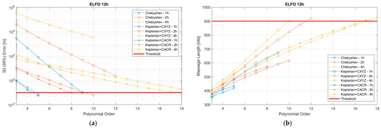
For comparison of the three main orbit models (Chebyshev polynomials, Keplerian plus correction in the Cartesian frame and Keplerian plus correction in the satellite frame), Figure 1 shows the 3D 95% error and the message length for the ELFO with 12 h validity. When the correction is applied on the satellite-body frame the accuracy is improved when using the same polynomial order due to the nature of the orbit perturbations. The impact of the orbit perturbations is more pronounced in the specific axes of the satellite-body frame (i.e., tangential/velocity direction (along-track direction) and radial direction) compared to the axes of a fixed reference frame. The corrections applied to the satellite-body frame will, therefore, model those perturbations more accurately. Furthermore, the number of bits necessary to represent the same polynomial order is slightly increased when the corrections are applied in the satellite-body frame, since the same polynomial order is applied in all three components (along, across, and radial), while this is not required to achieve the same/similar accuracy.

6. Discussion

The GNSS Keplerian orbit model is not able to represent the ELFO when the validity interval is close to the periapsis. The six basic Keplerian parameters can still be used to determine a reference satellite orbit with a low number of bits and low accuracy (in the order of meters).

The polynomial orbit models are very simple and provide high accuracy depending on the order used. The higher polynomial order, the higher the number of bits required to represent the orbit. The Chebyshev polynomials can be used with similar results [12,13] but have a lower number of bits due to their characteristics, specifically the range of polynomial being bounded from −1 to 1, in contrast to the traditional polynomials. The number of bits required to represent the orbit using pure polynomials is quite large because the orbit model must cope with a huge range of values for the Cartesian coordinates.

The novel orbit model presented in this paper shows a very good compromise between high accuracy and the number of bits. The binary representation of the orbit in this new model is reduced by using an initial reference orbit represented by the Keplerian model. The reference orbit allows the correction parameters of the Chebyshev polynomials to be much smaller than the ones obtained when using a pure Chebyshev polynomial orbit representation. By reducing the required number of bits, the correction polynomials can achieve higher orders and thus improve the accuracy of the orbit model.

The correction polynomials can be applied in two reference frames: Cartesian or satellite body. When applying the correction on the satellite frame, one can optimize the order of the polynomials in the different components (along, across and radial) by choosing different orders. This optimization allows for saving extra bits, and it will be presented in future work. Another important factor of this optimization relates to the orbit error projection to the user, which may have different impact (i.e., magnitude) on the different components; for example, in GNSS, the radial component is the driver of the orbit error projected into the user. Again, this optimization (as part of future work) will allow us to tailor the polynomial order to save additional bits.

The novel orbit model allows for the separation of the reference Kepler orbit from the polynomial correction in contrast to the pure polynomial approach. This separation might be important for future almanac representations, as one could use the same navigation message for the almanac.

7. Conclusions

In this paper, a novel orbit model was presented applicable to future LCNS orbits. The novel model outperforms the current orbit models (such as pure Keplerian models and pure polynomial models) in terms of accuracy by combining the Kepler orbit representation with a polynomial correction, it allows us to save additional bits to be used in higher-order polynomials.

8. Disclaimer

This publication does not cover the final Moonlight constellation, signals, and service but rather presents what could be achieved with a lunar navigation satellite system. The actual Moonlight constellation, signals, and related services will be defined as part of the ESA program outside this publication.

References

- Melman, F.M.; Zoccarato, P.; Orgel, C.; Swinden, R.; Giordano, P.; Ventura-Traveset, J. LCNS Positioning of a Lunar Surface Rover Using a DEM-Based Altitude Constraint. Remote Sens. 2022, 14, 3942. [Google Scholar] [CrossRef]
- Grenier, A.; Giordano, P.; Bucci, L.; Cropp, A.; Zoccarato, P.; Swinden, R.; Ventura-Traveset, J. Positioning and Velocity Performance Levels for a Lunar Lander using a Dedicated Lunar Communication and Navigation System. NAVIGATION J. Inst. Navig. 2022, 69, navi.513. [Google Scholar] [CrossRef]
- Molli, S.; Tartaglia, P.; Audet, Y.; Sesta, A.; Plumaris, M.; Melman, F.; Swinden, R.; Giordano, P.; Ventura-Traveset, J. Navigation Performance of Low Lunar Orbit Satellites Using a Lunar Radio Navigation Satellite System. In Proceedings of the 36th International Technical Meeting of the Satellite Division of The Institute of Navigation (ION GNSS+ 2023), Denver, CO, USA, 11–15 September 2023; Volume 36, pp. 4051–4083. [Google Scholar]
- LunaNet Interoperability Specification. Available online: https://www.nasa.gov/directorates/somd/space-communications-navigation-program/lunanet-interoperability-specification/ (accessed on 8 May 2024).
- European Commission. European GNSS (Galileo) Open Service Signal-In-Space Interface Control Document. Available online: https://www.gsc-europa.eu/sites/default/files/sites/all/files/Galileo_OS_SIS_ICD_v2.1.pdf (accessed on 24 April 2024).
- NAVSTAR GPS Space Segment/Navigation User Segment Interfaces, Interface Specification Document. Available online: https://www.gps.gov/technical/icwg/IS-GPS-200N.pdf (accessed on 24 April 2024).
- Van Dierendonck, A.J.; Russel, S.S.; Kopitzke, E.R.; Birnbaum, M. The GPS Navigation Message. J. Inst. Navig. 1978, 25, 147–165. [Google Scholar] [CrossRef]
- Tapley, B.D.; Schutz, B.E.; Born, G.H. Statistical Orbit Determination, 1st ed.; Elsevier Academic Press: Burlington, MA, USA, 2004; pp. 493–497. [Google Scholar]
- GODOT Documentation. European Space Agency. Available online: https://godot.io.esa.int (accessed on 26 June 2023).
- Bertone, S.; Arnold, D.; Girardin, V.; Lasser, M.; Meyer, U.; Jaggi, A. Assessing Reduced-Dynamic Parametrizations for GRAIL Orbit Determination and the Recovery of Independent Lunar Gravity Field Solutions. Earth Space Sci. 2021, 8, e2020EA001454. [Google Scholar] [CrossRef]
- Bury, G.; Zajdel, R.; Sosnica, K. Accounting for perturbing forces acting on Galileo using a box-wing model. GPSSolutions 2019, 23, 74. [Google Scholar] [CrossRef]
- Cortinovis, M.; Iiyama, K.; Gao, G. Satellite Ephemeris Approximation Methods to Support Lunar Positioning, Navigation, and Timing Services. In Proceedings of the 36th International Technical Meeting of the Satellite Division of The Institute of Navigation (ION GNSS+ 2023), Denver, CO, USA, 11–15 September 2023; Volume 36, pp. 3647–3663. [Google Scholar]
- Iess, L.; Di Benedetto, M.; Boscagli, G.; Racioppa, P.; Sesta, A.; De Marchi, F.; Cappuccio, P.; Durante, D.; Molly, S.; Plumaris, M.K.; et al. High Performance Orbit Determination and Time Synchronization for Lunar Radio Navigation Systems. In Proceedings of the 36th International Technical Meeting of the Satellite Division of The Institute of Navigation (ION GNSS+ 2023), Denver, CO, USA, 11–15 September 2023; Volume 36, pp. 4029–4050. [Google Scholar]
Disclaimer/Publisher’s Note: The statements, opinions and data contained in all publications are solely those of the individual author(s) and contributor(s) and not of MDPI and/or the editor(s). MDPI and/or the editor(s) disclaim responsibility for any injury to people or property resulting from any ideas, methods, instructions or products referred to in the content. |
© 2025 by the authors. Licensee MDPI, Basel, Switzerland. This article is an open access article distributed under the terms and conditions of the Creative Commons Attribution (CC BY) license (https://creativecommons.org/licenses/by/4.0/).