Abstract
In today’s world of large volumes of data, where the usual statistical estimation methods are commonly inefficient or, more often, impossible to use, aggregation methodologies have emerged as a solution for statistical inference. This work proposes a novel procedure for time series regression modelling, in which maximum entropy and information theory play central roles in the replication of time series, estimation of parameters, and aggregation of estimates. The preliminary results reveal that this three-stage maximum entropy approach is a promising procedure for time series regression modelling in big data contexts.
1. Introduction
Understanding, predicting, and interpreting information collected over different periods of time (days, weeks, years, etc.) has been of major concern in recent decades. Time series analysis, concerning longer or shorter periods, has been of major importance in various areas, such as economics and finance, agriculture, meteorology, astronomy, medicine, and health sciences, just to name a few. Current reality is characterized by large volumes of data, generally complex, unstructured and/or non-homogeneous, which are usually referred to as big data to emphasize the challenges they present to traditional computational and statistical techniques. In many situations, it is not possible to treat all data as a whole, either because of the inadequacy of the methodology or the insufficient computational capacity available. In such situations, traditional methods of estimation become inefficient and new statistical approaches are needed. The methodology adopted in this study was contextualized in the reality described above and is presented here as an alternative tool to deal with large volumes of data.
The strategy that is followed in this work is based on a three-stage maximum entropy approach for time series analysis. We started by considering a given data set to which the linear regression model could be applied, but represented a high computational burden when considering estimation. Instead of trying to tackle this issue using the whole data set, we started by considering only a few, say G, small samples or groups (with a few observations, say Obs) that were extracted from the original data using a random sampling procedure. The first step, after collecting the G small dimension random samples, was to replicate each of them following the maximum entropy bootstrap methodology proposed by H. D. Vinod [1,2]. Each replica could then be easily estimated using a proper estimation procedure. In the second stage, the generalized maximum entropy (GME) estimator was used to obtain estimates for the linear regression model parameters. Other estimators could have been considered in this stage, but due to the stability of the GME estimator in ill-posed problems (which are common in a big data context) this estimator was chosen for this work. Having an estimate for each parameter of the model and for each replica obtained of each original small sample, it was time to aggregate this information and obtain an overall estimate for each parameter of the model. Considering the total number of replicas, the percentile method can be used to obtain a confidence interval with any given confidence level for each of the model parameters (for a particular small sample of G groups collected). Alternatively, an overall estimate for each of the G group can be obtained by calculating the median of the estimates. As the normalized entropy is also calculated for each replica, the median normalized entropy can be obtained for each of the G samples. The third and last stage of the procedure consisted of aggregating the G estimates into one single estimate for each model parameter. To accomplish this last step, an entropy-based procedure was used once again, as the normalized entropy was used as the weighting factor for the aggregated overall model parameter estimate. Details about this aggregation technique, called neagging, can be found in [3,4]. This work reports the first time these three maximum entropy-based procedures have been combined into one single three-stage framework for regression analysis of time series. There are still many details that need further exploration, such as the adequate number of small samples or groups, G, and the proper number of observations per group, Obs, to consider; however, the preliminary results presented here are promising and certainly deserve to be brought to light.
2. Materials and Methods
This study considered daily available prices (USD; United States Dollar) for carbon dioxide (CO2) emissions, coal, natural gas, and Brent oil. Data from 2 July 2018 to 29 June 2022 were collected from Investing.com [5], considering only days with simultaneous information for all variables. The collected data for 994 days were considered a “big data set” that could only be analyzed using an aggregation methodology. Naturally, given the purpose of this work, the dimension was carefully chosen so that, although of high dimension, it was still computationally tractable, and the results of the model with 994 observations could be compared with those from the aggregation methodology. It is also important to note that the purpose of this work was not to provide an economic interpretation of the regression model defined below, but rather to illustrate how the combined methods may work in time series regression modelling scenarios. The methods considered in this work for replication of time series, estimation of parameters, and aggregation of estimates are briefly presented next.
2.1. Maximum Entropy Bootstrap for Time Series
The maximum entropy bootstrap for time series was proposed by H. D. Vinod [1,2]; a package (meboot) in the R software was developed by H. D. Vinod and J. López-de-Lacalle [6]. The methodology creates a large number of replicates of the time series for inference purposes (1000 replications were considered in this study). Those generated elements of the ensemble retain the shape of the original time series using maximum entropy density, as well as the time dependence structure of the autocorrelation and the partial autocorrelation functions. Moreover, and probably most importantly, the methodology avoids all structural changes and unit root type testing, and all the usual shape-destroying transformations, such as detrending or differencing, to achieve stationarity. Details of the algorithm can be found in [6].
2.2. Generalized Maximum Entropy Estimation
The GME estimator was proposed by A. Golan, G. Judge, and D. Miller [7] based on the maximum entropy (ME) principle of E. Jaynes [8,9] and the entropy measure of C. E. Shannon [10]. Recently, A. Golan [11] presented a new area of research at the intersection of statistics, computer science, and decision theory, entitled info-metrics, in which the GME estimator and other information–theoretic estimation methods are included. The GME estimator represents a stable estimation procedure in ill-posed models, namely in ill-conditioned models, in underdetermined models, and when only samples of small size are available for inference purposes (the micronumerosity problem).
Under GME estimation, the linear regression model , where denotes a () vector of noisy observations, is a () vector of parameters to be estimated, is a () matrix of explanatory variables, and is a () vector of random errors, needs to be reformulated as , where is a () matrix of support spaces, is a () matrix of support spaces, is a () vector of probabilities to be estimated, is a () vector of probabilities to be estimated, and and are the number of points in the support spaces. The GME estimator can then be stated as
subject to the model and the additivity constraints , and , where represents the Kronecker product. Using numerical optimization techniques, because the statistical problem has no closed form solution, the estimates of the parameters are given by . Additional details regarding GME estimation can be found in [7,11,12,13,14].
2.3. Normalized Entropy Aggregating (Neagging)
Aggregation methods become useful in big data contexts, where a significant computational effort is required and traditional statistical estimation methods become inefficient or, more often, impossible to apply. Normalized entropy aggregating (neagging) is based on identifying the information content of a given (randomly selected) group of observations () through the calculation of the normalized entropy; [3,4]. The aggregated (global) estimate is given by
where is the estimate in group , , with , and . Thus, neagging consists of weighting the estimates obtained from the GME estimator for each group according to the information content of the group.
2.4. Statistical Model and Estimation Configuration
The regression model is defined as
where represents the price of CO2 emissions, represents the price of coal, represents the price of natural gas, represents the price of Brent oil, represents the day, and is the error component.
First, maximum entropy bootstrap was used to create 1000 replications of the four series under study, using the package (meboot) in the R software [6]. Next, the four parameters of the 1000 models were estimated using the GME estimator (implemented in MATLAB by the authors) considering symmetric supports about zero in matrix , with five equally spaced points, and the following lower and upper bounds: , , and . The use of five supports was intended to illustrate different a priori information scenarios, and also to evaluate the performance of the estimation process. Regarding the matrix , the supports were defined symmetrically and centered on zero with three equally spaced points, using the three-sigma rule with the empirical standard deviation of the noisy observations, namely . With 1000 estimates for each parameter of the model in (3), the percentile method was used to construct confidence intervals for each one at 90%, 95%, and 99%. The twelve confidence intervals obtained from the 1000 models with 994 observations were then used to evaluate the performance of neagging.
Finally, to implement neagging in different scenarios, random sampling with replacement was performed considering two different number of groups, and , where the numbers of observations per group were 20 , 50 , and 100 . The parameters of the different models obtained by random sampling were estimated using the GME estimator with the same configuration mentioned above. As there were 1000 estimates and 1000 values of normalized entropy for each scenario, the median of the 1000 estimates was considered the estimate of each parameter, and the value of was obtained using the median (and the mean for comparison purposes; see next section) of the 1000 values of normalized entropy.
3. Results and Discussion
The results obtained in this work are summarized in Table 1, in which the rows contain the five different supports used: , , and . For each support, two different numbers of groups were tested, and . The number of observations per group is represented in the columns of Table 1, where the confidence intervals obtained by the percentile method for the confidence levels of 90%, 95%, and 99% are also listed. As these confidence intervals were calculated for each model parameter, we had twelve confidence intervals per support that related to the model with 994 observations. To evaluate results from the aggregation methodology, we checked if the overall aggregated confidence intervals, obtained for each of the random sampling scenarios listed in Table 1, had the same sign of the corresponding confidence interval. The best case scenario, evaluated for each of the 90 different scenarios tested, was four correct identifications of the corresponding confidence intervals signs (one for each model parameter), which we called four hits out of four. The worst case scenario would have been zero hits, which did not occur. Table 1 presents the number of hits for each scenario tested.

Table 1.
Number of hits in the comparison between confidence intervals for original data and overall confidence intervals for aggregated data.
The weighting of the estimates obtained from the GME estimator for each group according to the information content of the group—the neagging procedure—was done considering two alternative forms: using the median and the mean of the normalized entropy. The results are presented in a single table because they were exactly the same in terms of the number of hits. This equality of the median and the mean can be explained by the fact that the of the median and the mean were very close.
The discussion of the results in Table 1 has two focuses of analysis. The first one, looking at the lower amplitude supports , and , where it is expected that this lower amplitude comes from the fact that the user has a lot of information about the model (relating to a situation of a high a priori information), and the second one, looking at the supports and , with greater amplitude, where it is expected that the user has little information about the model (low a priori information scenarios).
In the first case, where the supports have smaller amplitude, it can be seen that with less observations per group (20 and 50), as the amplitude of the supports decreases, the number of hits increases and the results improve in cases where the aggregation is done with a smaller number of groups. However, the results are better for the scenario with 50 observations, when compared to the scenario with 20 observations. Finally, in the scenario with samples of 100 observations, the normalized entropy aggregation procedure presents 100% of hits in all supports , and , regardless of the number of groups.
For the second case, where we have little information about the model and the supports are of greater amplitude, whatever the support or , it can be seen that as the number of observations increases, the number of hits improves significantly, and for 50 and 100 observations it improves even more when the number of groups decreases from 10 to 5.
Therefore, in general, we can say that the results improve as the number of observations increase and the amplitude of the supports decrease, as well as the number of groups.
Looking at the highest density region (HDR) graphs below, which represent the model with 994 observations, we can see that the constant () in Figure 1 and the coefficient in Figure 2 are not statistically significant, as all confidence intervals (at confidence levels of 90%, 95%, and 99%) include zero. On the other hand, coefficients and can be considered statistically significant, as the corresponding confidence intervals do not include zero at any confidence level tested.
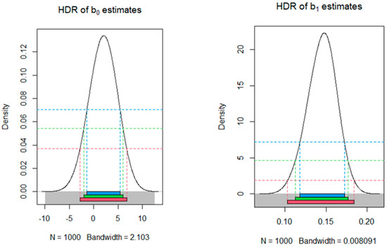
Figure 1.
HDRs for the sampling distribution of estimates of and .
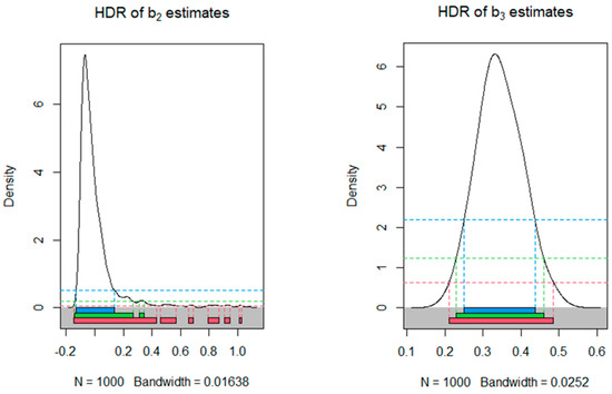
Figure 2.
HDRs for the sampling distribution of estimates of and .
Figure 3 shows the trend in the price of CO2 emissions. Figure 4 (on the left) shows trends in the price of coal, the price of natural gas, and the price of Brent oil in the period under study. Figure 4 (on the right) highlights only the price of natural gas, because it is not clear in the figure on the left.
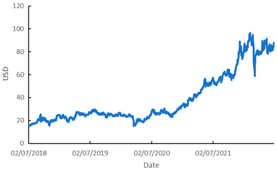
Figure 3.
Price of CO2 emissions.
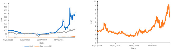
Figure 4.
Prices of coal, natural gas, and Brent oil (left), and the price of natural gas (right).
The values for all observed variables had an increasing trend, including the one represented separately in the graph on the right.
4. Conclusions
Recently, a two-stage maximum entropy approach for time series regression modelling was proposed in the literature [14]. This work extends that idea to big data contexts by adding a third stage with the neagging procedure. Although further research is needed, the preliminary results reveal that this three-stage approach, in which maximum entropy is used in replication of the time series, estimation of parameters, and aggregation of estimates, is a promising procedure in big data contexts. As future work, an exhaustive simulation study is being planned to investigate the adequate number of groups and the adequate number of observations per group. Additionally, comparisons with other aggregation methods, such as bagging, are expected to be analyzed, in order to explore the advantages and disadvantages of this three-stage approach.
Author Contributions
Conceptualization, methodology, software, investigation, data curation, writing—original draft preparation, and writing—review and editing: J.D., M.C. and P.M. All authors have read and agreed to the published version of the manuscript.
Funding
This work was supported by the Center for Research and Development in Mathematics and Applications (CIDMA) through the Portuguese Foundation for Science and Technology (FCT—Fundação para a Ciência e a Tecnologia), reference UIDB/04106/2020.
Institutional Review Board Statement
Not applicable.
Informed Consent Statement
Not applicable.
Data Availability Statement
Data collected from Investing.com (https://www.investing.com/, accessed on 5 August 2022).
Acknowledgments
We would like to express our gratitude to the Editor and two anonymous reviewers for all helpful comments.
Conflicts of Interest
The authors declare no conflict of interest.
References
- Vinod, H.D. Ranking mutual funds using unconventional utility theory and stochastic dominance. J. Emp. Financ. 2004, 11, 353–377. [Google Scholar] [CrossRef]
- Vinod, H.D. Maximum entropy ensembles for time series inference in economics. J. Asian Econ. 2006, 17, 955–978. [Google Scholar] [CrossRef]
- Costa, M.; Macedo, P. Normalized entropy aggregation for inhomogeneous large-scale data. In Theory and Applications of Time Series Analysis; Valenzuela, O., Rojas, F., Pomares, H., Rojas, I., Eds.; Springer: Cham, Switzerland, 2019; pp. 19–29. [Google Scholar] [CrossRef]
- Costa, M.; Macedo, P.; Cruz, J.P. Neagging: An aggregation procedure based on normalized entropy. In Proceedings of the International Conference on Numerical Analysis and Applied Mathematics, Rhodes, Greece, 17–23 September 2020; Simos, T.E., Tsitouras, C., Eds.; AIP Conference Proceedings: New York, NY, USA, 2022; Volume 2425, p. 190003. [Google Scholar] [CrossRef]
- Energy Prices 2022. Available online: https://www.investing.com (accessed on 5 August 2022).
- Vinod, H.D.; Lopez-de-Lacalle, J. Maximum entropy bootstrap for time series: The meboot R package. J. Stat. Softw. 2009, 29, 1–19. [Google Scholar] [CrossRef]
- Golan, A.; Judge, G.; Miller, D. Maximum Entropy Econometrics: Robust Estimation with Limited Data; Wiley: Chichester, UK, 1996. [Google Scholar]
- Jaynes, E.T. Information theory and statistical mechanics. Phys. Rev. 1957, 106, 620–630. [Google Scholar] [CrossRef]
- Jaynes, E.T. Information theory and statistical mechanics. II. Phys. Rev. 1957, 108, 171–190. [Google Scholar] [CrossRef]
- Shannon, C.E. A mathematical theory of communication. Bell Syst. Tech. J. 1948, 27, 379–423. [Google Scholar] [CrossRef]
- Golan, A. Foundations of Info-Metrics: Modeling, Inference, and Imperfect Information; Oxford University Press: New York, NY, USA, 2018. [Google Scholar] [CrossRef]
- Jaynes, E.T. Probability Theory—The Logic of Science; Cambridge University Press: Cambridge, UK, 2003. [Google Scholar] [CrossRef]
- Mittelhammer, R.; Cardell, N.S.; Marsh, T.L. The data-constrained generalized maximum entropy estimator of the GLM: Asymptotic theory and inference. Entropy 2013, 15, 1756–1775. [Google Scholar] [CrossRef]
- Macedo, P. A Two-Stage Maximum Entropy Approach for Time Series Regression. Commun. Stat. Simul. Comput. 2022; in press. [Google Scholar] [CrossRef]


Disclaimer/Publisher’s Note: The statements, opinions and data contained in all publications are solely those of the individual author(s) and contributor(s) and not of MDPI and/or the editor(s). MDPI and/or the editor(s) disclaim responsibility for any injury to people or property resulting from any ideas, methods, instructions or products referred to in the content. |
© 2023 by the authors. Licensee MDPI, Basel, Switzerland. This article is an open access article distributed under the terms and conditions of the Creative Commons Attribution (CC BY) license (https://creativecommons.org/licenses/by/4.0/).