Quantum Image Encoding Fidelity Metric (QIEF) for Performance Evaluation of Quantum Devices ^†

Abstract

The rapid advancement of quantum technologies has led to a growing and diverse landscape of quantum computing devices, each with varying architectures and capabilities. Most of them are evaluated using hardware-centric benchmarks such as gate fidelity, quantum volume, or coherence time. However, these metrics often fail to capture performance in problem-specific contexts, particularly in applications involving quantum image processing. In this work, we address this gap by introducing the Quantum Image Encoding Fidelity (QIEF) metric, a novel task-specific benchmark designed to evaluate how accurately quantum devices can encode classical image data into quantum representations. By focusing on image-specific criteria rather than device-agnostic parameters, QIEF offers a more application-relevant assessment of device capability, enabling a direct comparison of quantum hardware based on their effectiveness in real-world image-related tasks. We present the theoretical formulation of the QIEF, validate its relevance through quantum simulators and experiments on real quantum devices, and discuss its implications for guiding future hardware development tailored to quantum image processing applications.

1. Introduction

In the context of quantum computing for image processing, performance measurement can be approached from both software and hardware perspectives. Scientifically, we must consider the efficiency of quantum algorithms in terms of their ability to use the superposition and entanglement of qubits, as well as realization of the quantum circuits on the coupling maps of the real quantum devices.

From the software aspect, the representation of quantum images is crucial. The Flexible Representation of Quantum Images (FRQI) [1] is one approach for image encoding, which is essential for processing operations. However, the efficiency of the preparation process is low, indicating a need for algorithmic optimization to reduce the number of required qubits or gates.

On the hardware side, the performance is often measured by the number of qubits, the depth of quantum circuits, and the number of quantum gates required. For instance, a $2^n\times 2^n$ image requires with FRQI $2n+1$ qubits: 2n qubits to store pixel positions and one more qubit to store the intensity. The number of needed quantum gates is $(2^{4n}-3·2^{2n}+2n)$ [2], which is a huge number for larger images.

Algorithmic optimization is another key factor, where redesigning quantum algorithms to use fewer qubits or gates can inherently reduce circuit depth, leading to more efficient computation. Quantum computation uses the unique properties of qubits to perform calculations that classical computers cannot efficiently achieve, which is a significant advantage in processing large amounts of information in a compact and efficient manner.

In summary, for performance measurement of quantum computing in image processing, we should address the balance between the theoretical design of quantum algorithms and their practical implementation on quantum hardware, considering the trade-offs between computational efficiency and resource requirements.

2. Classical to Quantum Interface

To use quantum computing methods on classical data, like text, tabular data, or images, the data should first be transformed into quantum states, since classical formats are not directly compatible with quantum hardware. This step is called the encoding from classical data to quantum data, which means to represent the classical data in a way that is compatible with the quantum system for further manipulation [3]. It is also referred to as quantum data encoding, quantum feature mapping, quantum state preparation, or simply data embedding in quantum machine learning contexts. Although encoding data into a quantum system is more computationally demanding than in classical computing, it enables the use of quantum properties like superposition, entanglement, and interference. These properties can potentially offer a quantum advantage for certain tasks like optimization or pattern recognition [4]. In the case of gate-based quantum computing, the process is realized by quantum gates. These are the unitary operations that the quantum computer is designed to run for the preparation of the initial state of the computation [5]. Despite the enormous progress already made in quantum hardware, its power is still far from the corresponding classical computing, which inherently has difficulties such as high errors in operations per qubit, limited qubit quantity, short coherence time, permitted connectivity between qubits, and a few more constraints in the current NISQ era [6]. These constraint limit the possibility of quantum machine learning models and how they are developed at the moment. For instance, one popular method is to assign each feature in classical data to one qubit only and not use the full benefit of a proper encoding method. This option works effectively because the hardware constraints are balanced with the potential advantages of quantum computation [7]. The improvement of quantum hardware will such strategies to correspond with the potential of the quantum paradigm.

3. Quantum Hardware

Quantum hardware serves as the backbone for executing quantum computations, with various leading technologies currently in development. A notable method is superconducting quantum computing, which is utilized by companies such as IBM Quantum [8] and Google [9]. Superconducting quantum computers use superconducting circuits to form qubits, where quantum states are represented by oscillations within superconducting loops. These circuits function at extremely low temperatures, nearly absolute zero, to eliminate electrical resistance and enable coherent quantum states to persist. Qubits are manipulated using microwave pulses, and quantum gates are created by adjusting the energy levels of these superconducting qubits. These systems are highly scalable and can integrate well with existing classical electronics infrastructure. However, superconducting qubits are susceptible to errors due to their short coherence times and environmental noise, which requires sophisticated error-correction and/or error mitigation protocols to ensure reliable computations [10].

Another approach, used by companies like IonQ [11] and AQT [12], focuses on ion-based quantum computing. In these systems, individual ions, often trapped in electromagnetic fields, act as qubits. The quantum state of each ion is defined by specific electronic or nuclear spin-related energy levels, which are controlled using precisely tuned lasers. The ions are held in place by electromagnetic fields within a vacuum chamber, which helps isolate them from environmental disturbances. Quantum gates are implemented by applying laser pulses to create entanglement or to rotate the ion states. Ion-based systems are well known for their long coherence times and high gate fidelities, thanks to the inherent stability of ions. However, scalability poses a challenge, as increasing the number of qubits necessitates advanced ion-trapping setups and more complex control systems [13].

Comparing superconducting and ion-based quantum hardware highlights the trade-offs in performance and practicality. Superconducting systems are often preferred for their scalability and compatibility with existing semiconductor technologies, making them suitable for large-scale quantum computers. However, they encounter issues with coherence times and error rates, which require extensive error correction. On the other hand, ion-based systems are known for their stability and precision, featuring higher fidelity gates and longer coherence times. Nevertheless, their scalability is currently hindered by the challenges of managing large ion traps and the slower operational speeds of ion-based gates compared to superconducting ones. These differences indicate that while both technologies show potential, they may serve different applications or evolve into hybrid solutions in the future [6].

Beyond these, other promising quantum hardware platforms are being actively developed. Photonic quantum computers use individual photons as qubits, offering advantages such as room-temperature operation and easy transmission over long distances, making them attractive for quantum communication and network applications. Nitrogen-vacancy (NV) centers in diamond provide stable solid-state qubits with long coherence times at room temperature, useful for quantum sensing and certain computing tasks. Additionally, platforms like neutral atoms trapped in optical lattices, topological qubits based on exotic quasiparticles, and silicon-based spin qubits each bring unique benefits and challenges. As research progresses, it is likely that a diverse ecosystem of quantum technologies will coexist, with different hardware tailored to specific problem domains or combined in hybrid architectures to leverage their complementary strengths.

In this work, we primarily use IBM’s superconducting quantum computers. Among the various platforms available—such as those from Google, Rigetti, and IQM—we chose IBM’s quantum hardware due to its seamless accessibility via the cloud, which allows for direct, remote usage of real quantum processors without the need for local infrastructure or maintenance. This cloud-based access, along with IBM’s close collaboration with research institutions like Fraunhofer, enabled us to conduct experiments frequently and reliably.

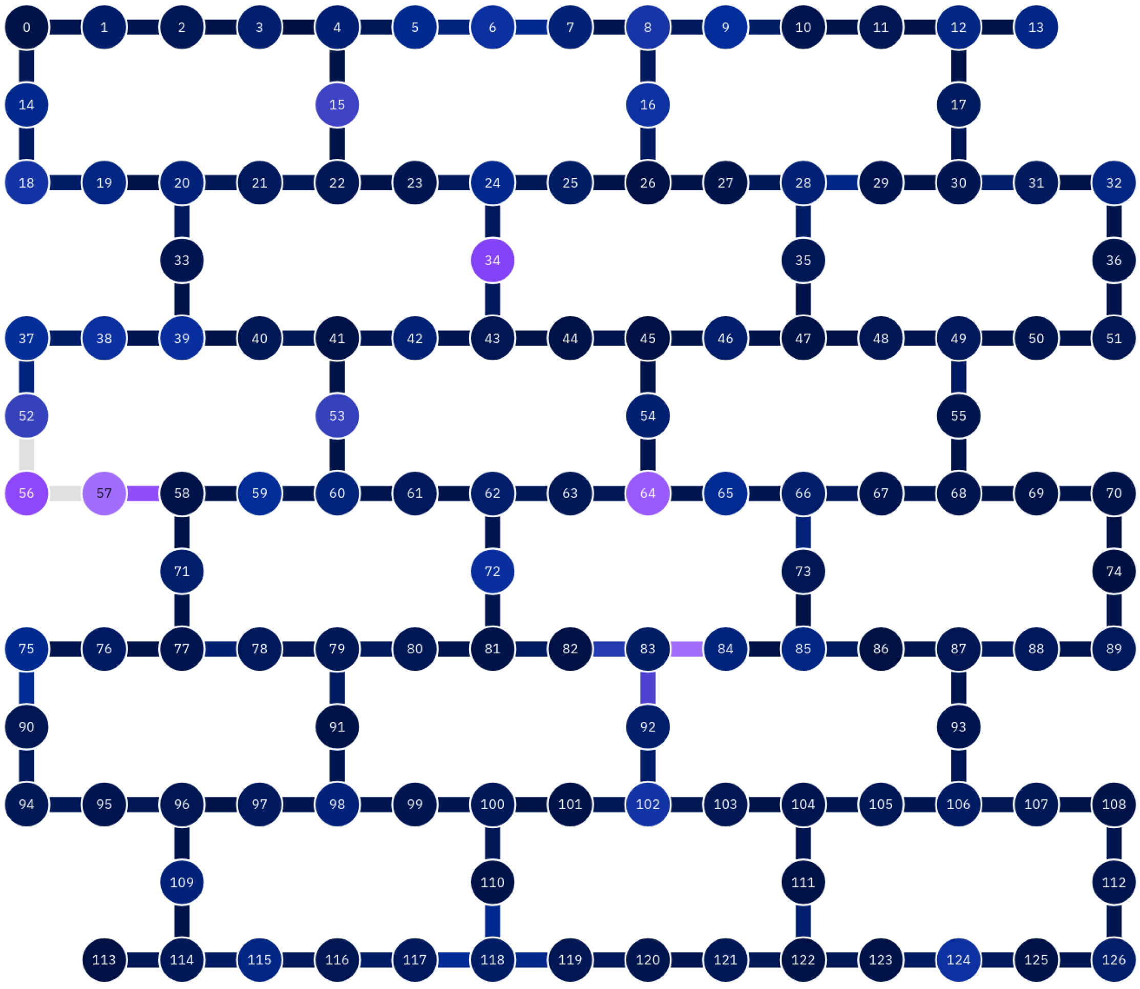
IBM’s transparency and the level of detail in its hardware performance were also important factors in our decision. Each quantum backend is accompanied by regularly updated calibration data, including coupling maps, gate error rates, readout errors, and coherence times. This data allows for optimization of circuit compilation and backend selection if needed. For instance, coupling maps—such as the one shown in Figure 1—depict the physical connectivity of qubits.

Lines between qubits indicate two-qubit gate connections or a so-called Echoed Cross-Resonance gate (ECR), and their colors reflect the corresponding error rates. The node colors represent readout errors associated with individual qubits, providing valuable insights for algorithm and circuit design. This visualization can be used to guide the selection and placement of qubits, ultimately contributing to improved overall fidelity and more robust quantum circuit implementations.

Table 1. Calibration data of IBM backends taken on 15 July 2025. The values are median values. The error rates of 2-qubit gates (here ECR- or CZ-error), 1-qubit gates (SX-error), and readout error are given in %.

Backend	2-Qubit	1-Qubit	Readout	T1 (µs)	T2 (µs)
ibm_brussels	0.8013	0.0232	2.7100	263.82	188.25
ibm_strasbourg	0.6930	0.0293	1.880	309.67	161.07
ibm_aachen	0.1977	0.0211	0.7568	214.74	181.18
ibm_sherbrooke	0.5743	0.0214	2.1480	264.28	211.71
ibm_brisbane	0.6646	0.0234	1.8800	242.80	129.75
ibm_torino	0.2742	0.0315	2.1970	173.55	136.53
ibm_marrakesh	0.2555	0.0309	0.7813	195.83	101.55
ibm_kingston	0.2178	0.0240	0.7568	271.43	153.47
ibm_fez	0.2770	0.0294	0.8301	143.82	98.00

shows the current backend-specific calibration metric values of IBM’s quantum devices used in this paper.

Table 2. Metadata of IBM backends taken on 15 July 2025.

Backend	Qubits	CLOPS	Processor Type	Region
ibm_brussels	127	220 K	Eagle r3	eu-de
ibm_strasbourg	127	220 K	Eagle r3	eu-de
ibm_aachen	156	250 K	Heron r2	eu-de
ibm_sherbrooke	127	150 K	Eagle r3	us-east
ibm_brisbane	127	180 K	Eagle r3	us-east
ibm_torino	133	210 K	Heron r1	us-east
ibm_marrakesh	156	195 K	Heron r2	us-east
ibm_kingston	156	250 K	Heron r2	us-east
ibm_fez	156	195 K	Heron r2	us-east

shows metadata and performance data of the quantum devices, like the number of qubits and Circuit Layer Operations Per Second (CLOPS). For the most up-to-date specifications of the quantum backends, we refer to IBM’s quantum website [8].

4. Quantum Simulators

Quantum simulators are essential in the field of quantum computing, as they allow researchers to simulate quantum circuits on classical hardware. This capability enables the development and testing of quantum algorithms without needing physical quantum devices. IBM’s Qiskit features the Qiskit Aer Quantum Assembly Language (qasm_simulator), a low-level, human-readable language and powerful tool for developing quantum circuits. This simulator can emulate noisy quantum systems by integrating error models, which helps conduct experiments under conditions that mimic real hardware. It is capable of handling large-scale circuits, making it ideal for prototyping quantum algorithms prior to executing them on IBM Quantum devices. Similarly, the AQT (Alpine Quantum Technologies) simulator aqt_qasm_simulator provides a strong platform for emulating ion-trap quantum computers. AQT’s simulator delivers high-fidelity simulations of circuits specifically designed for ion-based systems, emphasizing precise control and noise modeling that is tailored to their unique hardware architecture. For a more detailed description, we refer to the official websites of the respective quantum computing providers [8,12].

On the other hand, Pennylane [14], an open-source software library for quantum machine learning, offers two key simulators: pennylane_default.qubit and the alternative pennylane_lightning.qubit. The pennylane_default.qubit simulator utilizes a dense state-vector representation to emulate quantum circuits, making it adaptable and ideal for hybrid quantum-classical workflows.

In contrast, the second option pennylane_lightning.qubit employs C++ backends for enhanced performance, allowing for the efficient simulation of larger circuits with high accuracy. Both simulators integrate smoothly into the Pennylane framework, supporting advanced features such as automatic differentiation for optimizing quantum machine learning models.

These simulators collectively form an essential part of the quantum ecosystem, addressing specific aspects of quantum computing—from noise modeling to performance optimization—accelerating the development and understanding of quantum algorithms.

Comparison of Quantum Simulators

Quantum simulators vary in their architecture, focus, and performance traits as shown in

Table 3. Comparison of representative quantum simulators and their main features.

Simulator	Provider	Key Feature	Specialization	Performance
qasm simulator	IBM	Noise modeling for IBM hardware	General quantum circuits	Moderate speed, high realism
aqt_qasm simulator	AQT	High fidelity for ion-trap systems	Ion-trap architectures	High accuracy, ion-specific
pennylane default	PennyLane	Dense state-vector simulation	Hybrid quantum-classical	General-purpose, flexible
pennylane lightning	PennyLane	Optimized C++ backend for speed	Large-scale statevector circuits	High speed, high precision

. Qiskit’s qasm_simulator is designed to simulate noise and is compatible with IBM’s quantum devices, making it ideal for studying realistic conditions in quantum hardware. AQT’s simulator aqt_qasm_simulator is tailored for ion-trap architectures, providing high fidelity and accuracy specifically for ion-based systems. Pennylane’s pennylane_default.qubit offers a flexible state-vector simulation that works well for hybrid quantum-classical workflows, while pennylane_lightning.qubit focuses on speed and precision, utilizing an optimized C++ backend for large-scale circuits. These differences ensure that each simulator is well suited for various research and application requirements.

5. Boundaries, Limitations, and Abilities of Real Quantum Hardware and Simulators

Quantum simulators, which operate on classical hardware, serve as crucial platforms for developing, testing, and refining quantum algorithms. Tools like IBM’s Qiskit qasm_simulator or Pennylane’s pennylane_default.qubit enable accurate modeling of quantum systems, including noise and gate imperfections, allowing researchers to experiment under realistic quantum conditions. However, simulators are constrained by the exponential growth of classical memory and processing needs, which limits their ability to emulate systems with a large number of qubits.

The Nyquist–Shannon sampling theorem [15], which is usually associated with signal processing, is also important in quantum computing for processes such as quantum state tomography and quantum sampling. It states that to accurately reconstruct a quantum state or distribution, a sufficient number of samples must be taken, which depends on the complexity of the state. In noisy quantum systems, this implies that the number of shots required to obtain meaningful results can increase exponentially with the size and depth of the quantum circuit.

Real quantum hardware is theoretically capable of providing remarkable computational power based on principles of quantum mechanics such as superposition, entanglement, and interference. However, it faces considerable physical and technological challenges. The main limitations arise from hardware imperfection, including high noise levels, short coherence times, qubits connectivity, and operations with high error rates. These factors limit the depth of quantum circuits that can be run before errors overwhelm the computation. Additionally, the small number of qubits in existing quantum systems restricts the execution of large-scale algorithms, confining practical applications to proof-of-concept demonstrations or specific tasks like quantum-enhanced optimization and small-scale simulations.

Current noise levels differ across hardware platforms, but typical two-qubit gate fidelities are around 99% for superconducting qubits (see, for example, Table 1) and slightly higher for ion-trap systems. These imperfections greatly affect the reliability of the results, which makes error mitigation or correction techniques essential. Additionally, access to quantum hardware is often restricted due to high demand, resulting in long wait times for execution on cloud-based platforms like IBM Quantum or Rigetti. These limitations highlight the critical role of simulators for immediate experimentation and algorithm development.

Despite these obstacles, the potential to use quantum computing offers the promise of solving problems that are intractable for classical computers, positioning quantum hardware as a key element of future computing.

The execution time on real quantum hardware includes both the actual computation time and various overhead factors. Physical execution is incredibly fast, typically taking microseconds or nanoseconds for each gate operation. However, the overhead can include delays from queuing, time for initialization and calibration, data transfer, and post-processing, which can significantly extend the total computation time. However, simulators run entirely on classical hardware, where execution times are influenced by the available classical computational resources. Although simulators can face considerable overhead for larger systems due to exponential scaling, they provide deterministic execution times, making them more suitable for iterative algorithm development.

Both real quantum hardware and classical simulators have distinct boundaries, limitations, and capabilities. Striking a balance between quantum hardware and simulators is essential for progressing quantum computing research and creating applications that fully use this emerging field. We build this balance between simulation and real hardware into our methodology.

6. Methodology

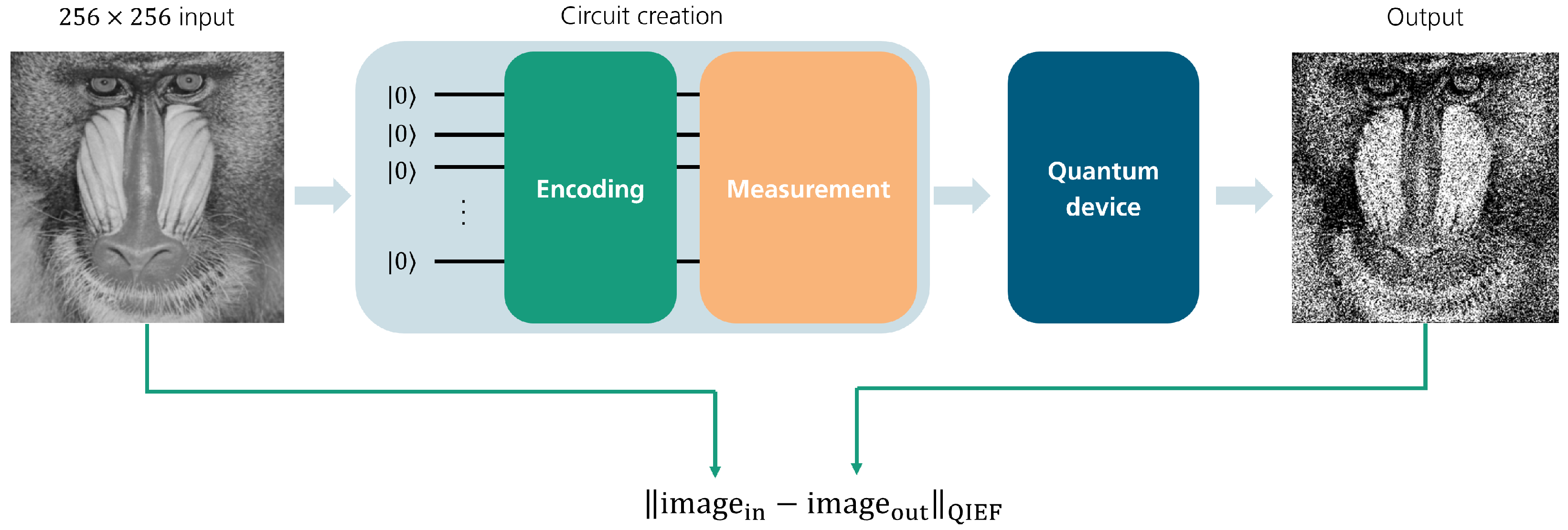
Figure 2 shows an overview of our experimental setup. The process starts with a classical image, which can be either in grayscale or RGB format, serving as the input data. This image undergoes an encoding procedure that converts the classical pixel values into quantum states. This encoding step is essential as it prepares the data for processing within the quantum computing framework. The method chosen for encoding plays a crucial role in how the classical information is mapped onto quantum states, significantly influencing the accuracy and efficiency of the computation. The circuit creation is then finished by applying measurements to all qubits.

The prepared quantum circuit is then deployed on either a real quantum hardware platform or a quantum simulator. Real quantum hardware runs the circuit using physical qubits, enabling the experiment to utilize quantum phenomena such as superposition and entanglement. On the other hand, quantum simulators replicate the behavior of a quantum system on classical hardware, offering a more affordable and accessible option for experimentation. The choice of execution platform has a significant impact on the results due to variations in hardware noise, coherence times, and other factors.

After the execution is complete, the output quantum states are processed to recreate the image in a classical format. This post-processing step involves translating the quantum measurements back into pixel values, which allows for a direct comparison between the original image ${\mathrm{image}}_{\mathrm{in}}$ and the reconstructed one ${\mathrm{image}}_{\mathrm{out}}$. This comparison is essential for assessing how effective an encoding method is. We call the difference between the original and reconstructed images Quantum Image Encoding Fidelity (QIEF). As an example, the normalized L1 norm can be used for that

$$\begin{array}{cc}\hfill {\parallel ·\parallel }_{{\mathrm{QIEF}}_{\mathrm{nL}1}}& ={\displaystyle \frac{100}{255}}\left|{\mathrm{image}}_{\mathrm{in}}-{\mathrm{image}}_{\mathrm{out}}\right|\hfill \\ \hfill & ={\displaystyle \frac{100}{255}}{\displaystyle \frac{1}{N}}\left|{\displaystyle \sum _{i=1}^N}\left({\mathrm{image}}_{\mathrm{in}}\left(i\right)-{\mathrm{image}}_{\mathrm{out}}\left(i\right)\right)\right|,\hfill \end{array}$$

(1)

where the value 100 in the equation is for having the results in %.

Identifying the whole process from image encoding, measuring the quantum states and reconstructing the image as Quantum Image Encoding Fidelity provides a clear and quantifiable indication of how well the quantum system maintains the original image data throughout the processes of encoding, execution, and decoding. Additionally, the fidelity reveals the effects of noise, hardware limitations, and encoding strategies, offering important insights into the strengths and weaknesses of the quantum platform.

In the context of comparing binary and gray-value images, various distance formulas serve as fundamental tools for quantifying the similarity between two images. For binary images, metrics like the Hamming distance are commonly employed, which counts the number of differing pixel values between two images. This simple yet effective approach provides a straightforward measure of similarity. For gray-value images, however, more sophisticated formulas are required to account for varying intensities. The Mean Squared Error (MSE) is a widely used metric that calculates the average squared difference between the corresponding pixel values of two images [16]. It is defined as follows:

$$\mathrm{MSE}={\displaystyle \frac{1}{N}}{\displaystyle \sum _{i=1}^N}{\left({\mathrm{image}}_{\mathrm{in}}\left(i\right)-{\mathrm{image}}_{\mathrm{out}}\left(i\right)\right)}^2,$$

(2)

where N is the total number of pixels in the image, ${\mathrm{image}}_{\mathrm{in}}\left(i\right)$ is the intensity of the i-th pixel in the input image, and ${\mathrm{image}}_{\mathrm{out}}\left(i\right)$ is the corresponding pixel intensity in the processed image. While intuitive, MSE emphasizes larger differences due to its quadratic nature, making it sensitive to outliers.

An extension of the MSE is the Peak Signal-to-Noise Ratio (PSNR), which is often used to assess the quality of reconstructed images [16]. PSNR is expressed in decibels (dB) and compares the maximum possible pixel intensity in the image to the MSE. Higher PSNR values indicate greater similarity between the original and reconstructed images. Specifically, PSNR is defined as follows:

$$\mathrm{PSNR}=10·{log}_{10}\left({\displaystyle \frac{{\mathrm{MAX}}^2}{\mathrm{MSE}}}\right),$$

(3)

where MAX is the maximum pixel value in the image, typically 255 for 8-bit images. PSNR is particularly valuable in scenarios where perceptual quality needs to be evaluated, as it provides a standardized measure of reconstruction fidelity.

7. Quantum Image Encoding Methods

Encoding classical images into quantum states is a fundamental prerequisite for quantum image processing. This section reviews the principal encoding techniques—basis, amplitude, and phase encoding—and discusses specific methods such as QBIP [17], QPIE [18], FRQI-MCRY [1], FRQI-MARY [2], and NEQR [19], including recent improvements for NISQ hardware.

7.1. Basis Encoding

Basis encoding maps classical information directly onto the computational basis states of a quantum system. Formally, an n-bit string $x=x_1{x}_2\dots x_n$ is encoded as follows:

$$|x\rangle =|x_1\rangle \otimes |x_2\rangle \otimes \cdots \otimes |x_n\rangle .$$

(4)

Quantum Boolean Image Processing (QBIP) [17] follows this principle by representing binary image pixels using basis states. This method benefits from operational simplicity but requires a number of qubits proportional to the image size, making it unsuitable for large images on current quantum devices. For further details, we refer to the original paper [17] or our previous work [20].

7.2. Amplitude Encoding

Amplitude encoding encodes normalized pixel values into the amplitudes of a quantum state. A classical image vector $I\in {\mathbb{R}}^{2^n}$ is mapped as follows:

$$|\psi \rangle ={\displaystyle \sum _{i=0}^{2^n-1}}{I}_i|i\rangle ,$$

(5)

where ${\sum }_{i=0}^{2^n-1}{\left|I_i\right|}^2=1$. Quantum Probability Image Encoding (QPIE) [18] implements this strategy, enabling efficient storage and manipulation of image data. While amplitude encoding is qubit-efficient and, for example, natively implemented in Qiskit via the circ.initialize(state) command, extracting full information from the quantum state remains challenging due to the probabilistic nature of quantum measurements. For further details, we refer to the original paper [18] or our previous work [20].

7.3. Phase Encoding

In phase encoding, classical information is encoded into the phase of a quantum state. In the Flexible Representation of Quantum Images (FRQI) [1], a grayscale image is represented as follows:

$$|{\psi }_{\mathrm{FRQI}}\rangle ={\displaystyle \frac{1}{2^n}}{\displaystyle \sum _{i=0}^{2^n-1}}\left(cos\left({\theta }_i\right)|0\rangle +sin\left({\theta }_i\right)|1\rangle \right)\otimes |i\rangle ,$$

(6)

where ${\theta }_i$ corresponds to the grayscale value at position i, ${\theta }_i\in \left[0,{\displaystyle \frac{\pi }{2}}\right]$.

Multi-Controlled Ry rotation gates are used to implement the rotations (FRQI-MCRY). However, FRQI-MCRY still requires a substantial number of CX gates. The Multi-Adapted Ry Rotation (FRQI-MARY) approach [20,21] improves upon this by reducing the number of CX gates approximately by half, enhancing scalability on NISQ devices. For further details, we refer to the original paper [1] or our previous work [20].

7.4. Alternative Encoding: NEQR

The Novel Enhanced Quantum Representation (NEQR) [19] offers a different paradigm by encoding pixel grayscale values directly into computational basis states. For a grayscale pixel value $g_i$ represented as a binary sequence $(g_{i,0},g_{i,1},\dots ,g_{i,m-1})$, NEQR defines the following:

$$|I\rangle ={\displaystyle \frac{1}{2^n}}{\displaystyle \sum _{i=0}^{2^n-1}}|g_{i,0}{g}_{i,1}\dots g_{i,m-1}\rangle \otimes |i\rangle .$$

(7)

While NEQR provides deterministic pixel retrieval, it requires deeper quantum circuits with numerous multi-controlled operations, posing challenges for current quantum hardware.

For more information about quantum image encoding methods and further encoding methods we refer to [2,20,22,23,24,25].

Overall, these encoding methods each offer trade-offs between qubit resources, circuit depth, and noise resilience, shaping the practical use of quantum image processing in the NISQ era. We refer to [20] for more details and a comparison of these encoding methods from perspectives like the number of qubits, transpiling time, or maximum executable image size.

8. Application and Experiments

To evaluate the effectiveness of the Quantum Image Encoding Fidelity (QIEF), we present the performance of the aforementioned quantum image encoding methods along with their corresponding metrics, demonstrated through a variety of image examples. In addition to a $2\times 2$ sample image, we also test the methods on a commonly used $256\times 256$ image processing sample Mandrill (Baboon) from the USC-SIPI Image Database [26]. To ensure compatibility with the requirements of various simulators and real quantum backends, certain assumptions were made in the experimental setup, enabling a fair comparison of the results across different platforms.

Since parts of the experimental setup were previously reported in [20] and the implementation was primarily developed using Qiskit, it became necessary to adapt the code for compatibility with PennyLane. Two approaches were considered for this adaptation: (1) exporting the Qiskit circuits to a QASM file and subsequently importing them into PennyLane or (2) re-implementing the code directly within the PennyLane framework. To avoid the additional overhead associated with generating, storing, and reloading QASM files, we opted for the latter approach. This required the manual translation of several aspects as summarized in

Table A1. Comparison between Qiskit (1.x) and PennyLane (0.45.1) workflows.

Aspect	Qiskit	PennyLane
Circuit Construction	Uses QuantumCircuit, QuantumRegister, ClassicalRegister	Uses @qml.qnode decorated Python (v3.11) functions to define circuits
Measurement	Uses measure_all() and classical registers	Uses return qml.sample(...)
Execution	Uses backend.run(), execute(), job.result()	Directly calls QNode as a function (e.g., output = qnode())
Backend Setup	Uses Aer.get_backend(...) or real IBMQ backends	Uses qml.device("default.qubit", wires=..., shots=...)
Transpiling	Requires transpile(circuit, backend)	No transpiling required
Multi-Control Gates	Uses mcx(), mcry(), supports ancilla qubits	Uses qml.MultiControlledX(), manual wire configuration
Drawing Circuits	Uses circuit.draw(’mpl’)	Uses qml.draw_mpl(qnode)()
Multiple Circuits (Bitplanes)	List of QuantumCircuit objects	List of QNodes or inline QNode construction with loop-local variables
Avoiding Named QNodes	Not applicable	Use inline functions or closures
Postprocessing Counts	Uses result.get_counts() (dictionary output)	Returns NumPy array of samples; use np.bincount() or similar
Error Fixes	–	Removed invalid QuantumCircuit, fixed control wires/values in multi-controlled gates, ensured each bitplane circuit is correctly generated without overwriting

.

For the calculation, we used a computer with an Intel(R) Xeon(R) Gold 6442Y processor running at maximum 4 GHz, a total RAM of 502 GB, and Red Hat Enterprise Linux 9.5 (Plow).

8.1. Sample Image of Size 2 × 2

Due to the limitations of certain methods and hardware providers in handling larger images, a $2\times 2$ sample image with pixel intensity values $\{10,85,170,255\}$ was selected. This image spans the full grayscale range and serves as a representative test case. The objective is to compare both the encoding methods and the performance of different simulators or physical quantum hardware. The evaluation criteria include circuit creation time, execution time, and quantum image encoding fidelity, assessed using multiple metrics.

Since AQT currently has the most limiting maximum number of shots with $n\_shots=2000$, we use this number as value for comparison for all methods and other providers.

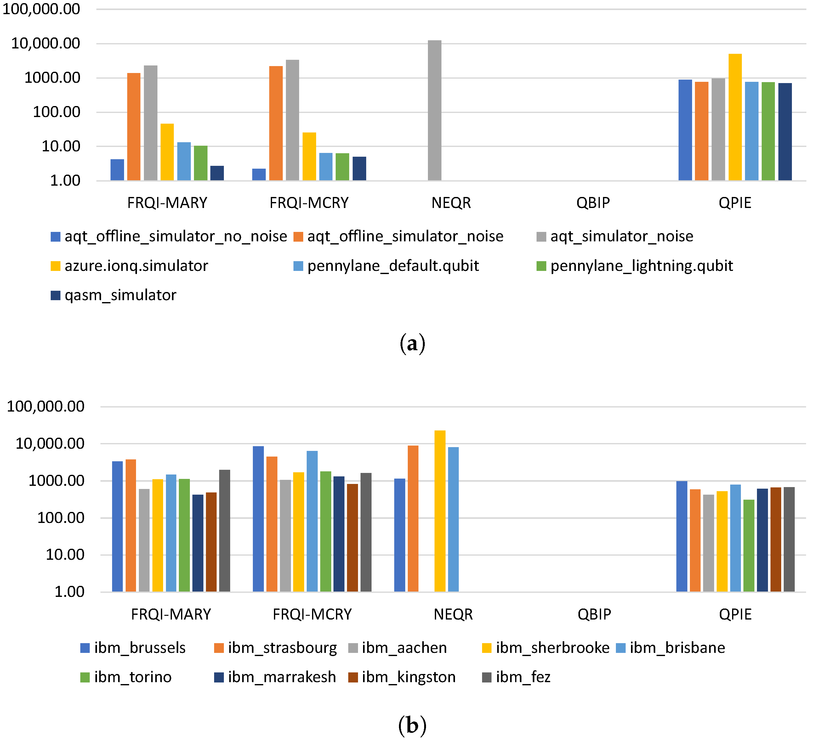
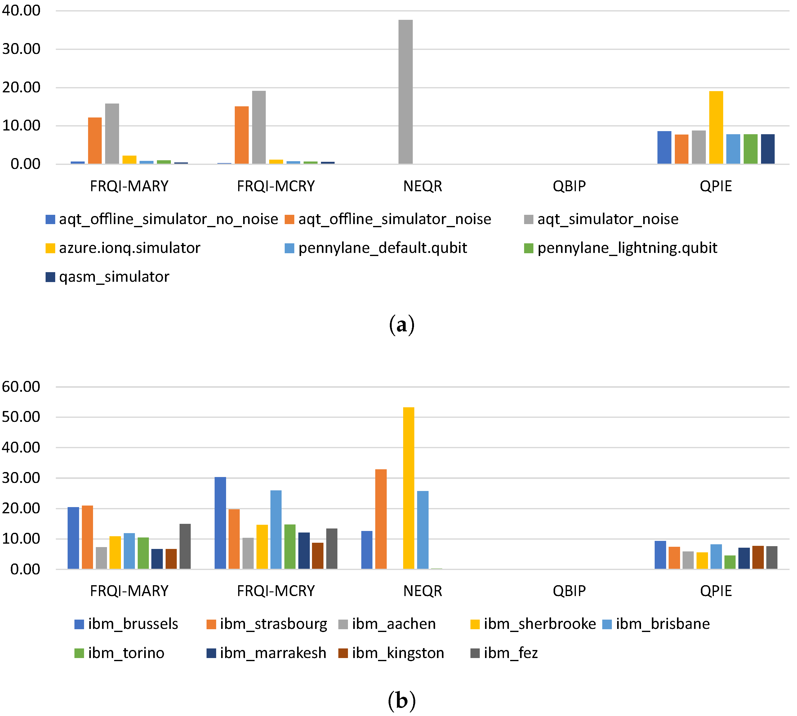
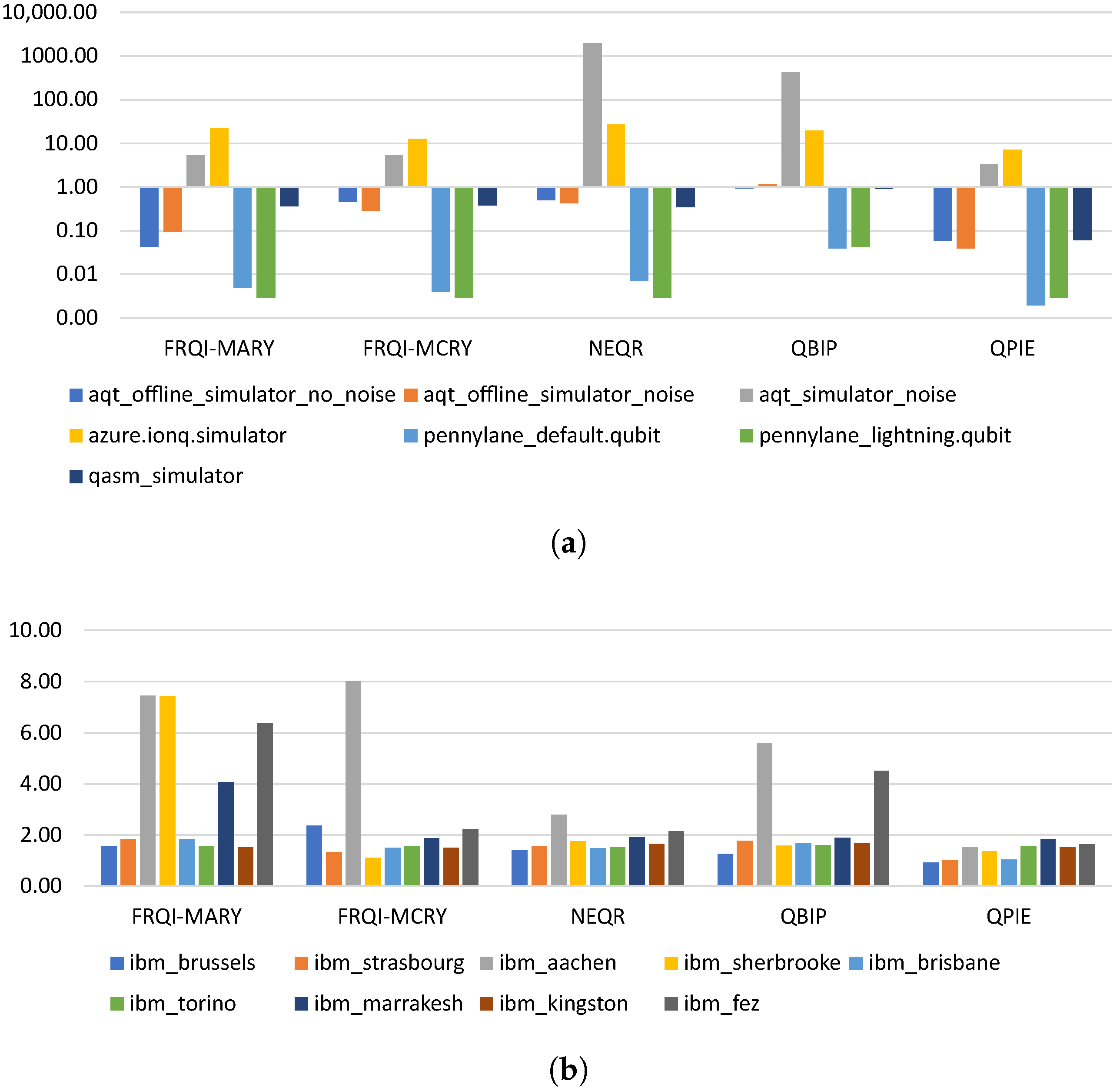
The results of the sample image are visualized in Figure 3, Figure 4, Figure 5 and Figure 6 where we compare the performance ${\parallel ·\parallel }_{{\mathrm{QIEF}}_{\mathrm{nL}1}},{\parallel ·\parallel }_{{\mathrm{QIEF}}_{\mathrm{MSE}}},{\parallel ·\parallel }_{{\mathrm{QIEF}}_{\mathrm{PSNR}}}$ and the required execution times needed to calculate the results.

It is visible that with the NEQR and QBIP methods there is, in most cases, no deviation to the original input image. That means we can reconstruct the image again as we had before encoding the image. With both the amplitude encoding method QPIE and the phase encoding method FRQI, we see the deviation from the original image. This lies in the type of encoding and in the conversion of the measurements to the classical pixel values [20].

Between the simulators we also see the clear difference between the AQT noiseless and the noisy versions in FRQI. The fact that the QPIE is similar whether noiseless or noisy highlights the difficulty of retrieving the image from the amplitudes of the quantum states (see also in [20]).

For the earlier staged real quantum backends with processor type Eagle r3, like ibm_brussels, ibm_strasbourg, ibm_sherbrooke, and ibm_brisbane, we observe results that are comparable to those obtained using the noisy configuration of the AQT simulator. This similarity can be primarily attributed to inherent noise in the quantum gate operations, limited coherence times, crosstalk between qubits, and other hardware-level inconsistencies present in the current NISQ quantum devices.

The newer processor types Heron r1 and r2 (ibm_aachen, ibm_torino, ibm_marrakesh, ibm_kingston, and ibm_fez) show better performance. This is clearly visible for the NEQR method in Figure 3, Figure 4, Figure 5 and Figure 6. While the Eagle r3 backends exhibit substantial errors, the QIEF values obtained with the newer processor types are optimal, enabling complete image reconstruction. This effect can be attributed to the improved error rates resulting from the use of CZ-gates as native two-qubit gates, in contrast to ECR-gates (see Table 1). The error rates per two-qubit gate are reduced by at least half, and in some cases, even more significantly.

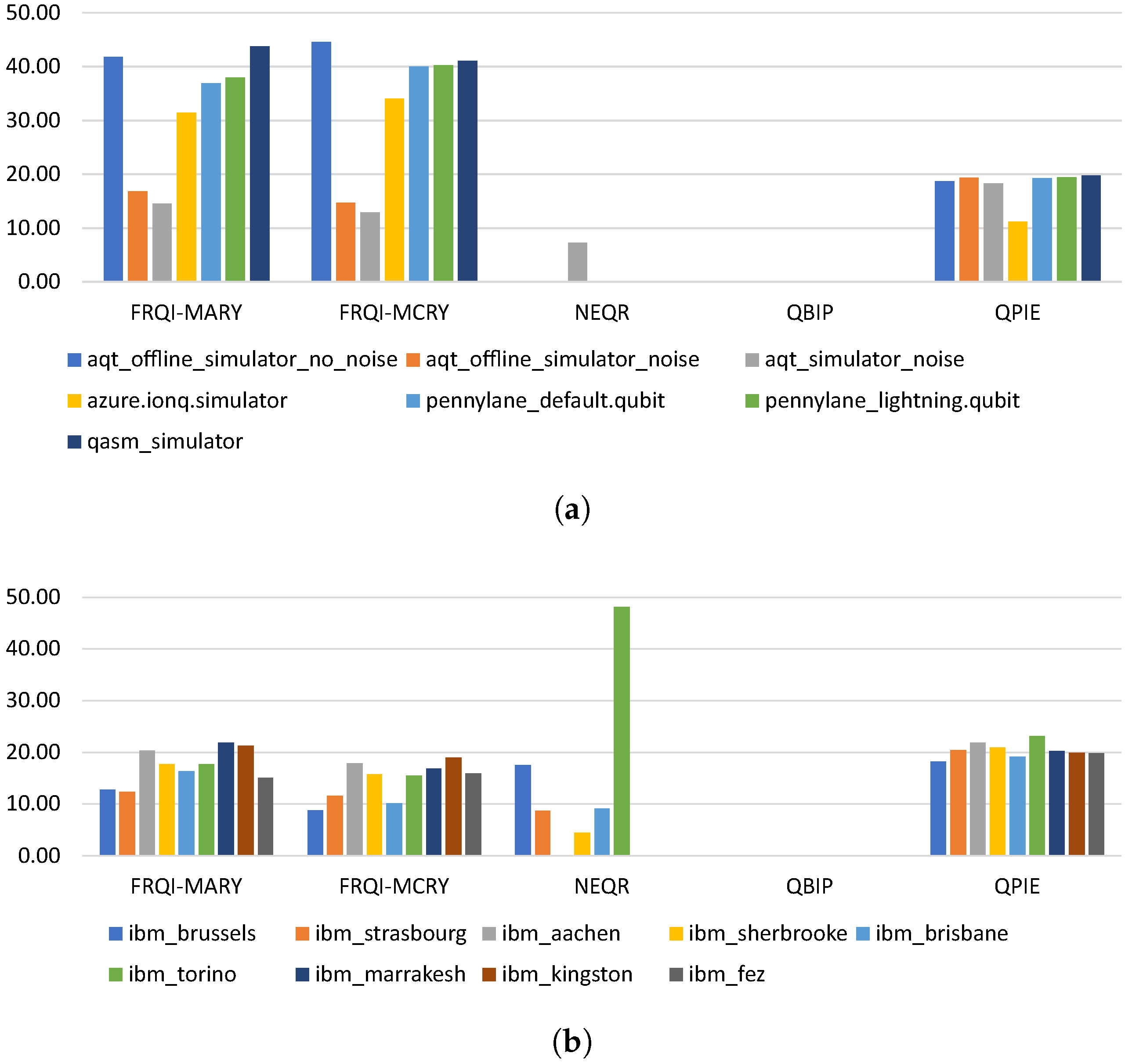
The execution times presented in Figure 6a highlight the relative performance differences among the evaluated simulation backends. Notably, pennylane_default.qubit and pennylane_lightning.qubit from the PennyLane framework exhibit marginally superior performance in terms of execution time when compared to qasm_simulator, aqt_offline_simulator_no_noise and aqt_offline_simulator_noise. Furthermore, the third AQT simulator aqt_simulator_noise and azure.ionq.simulator backends demonstrate a clearly increased computational overhead, reflecting the additional complexity introduced by noise modeling or remote execution infrastructure.

For the real quantum backends, we report the execution times obtained from actual hardware executions, as shown in Figure 6b. These values are slightly higher compared to those from the qasm_simulator and PennyLane’s simulators, primarily due to the inherent noise in physical quantum systems and the overhead introduced by remote execution. It is important to note that the reported results do not account for queuing times, which can vary depending on system availability, personal access, and load. In practice, total execution time may be significantly affected by fair-share queuing policies enforced by quantum computing providers or the need to manually start the jobs and synchronize with the hardware provider.

8.2. Sample Images of Size 256 × 256

To further validate the applicability of our approach, we evaluated it on a well-established benchmark image Mandrill (Baboon) from the USC-SIPI Image Database [26], which is commonly used in classical image processing. We resized it to a resolution of $256\times 256$ using a Gaussian kernel in ToolIP (version 2025) [27].

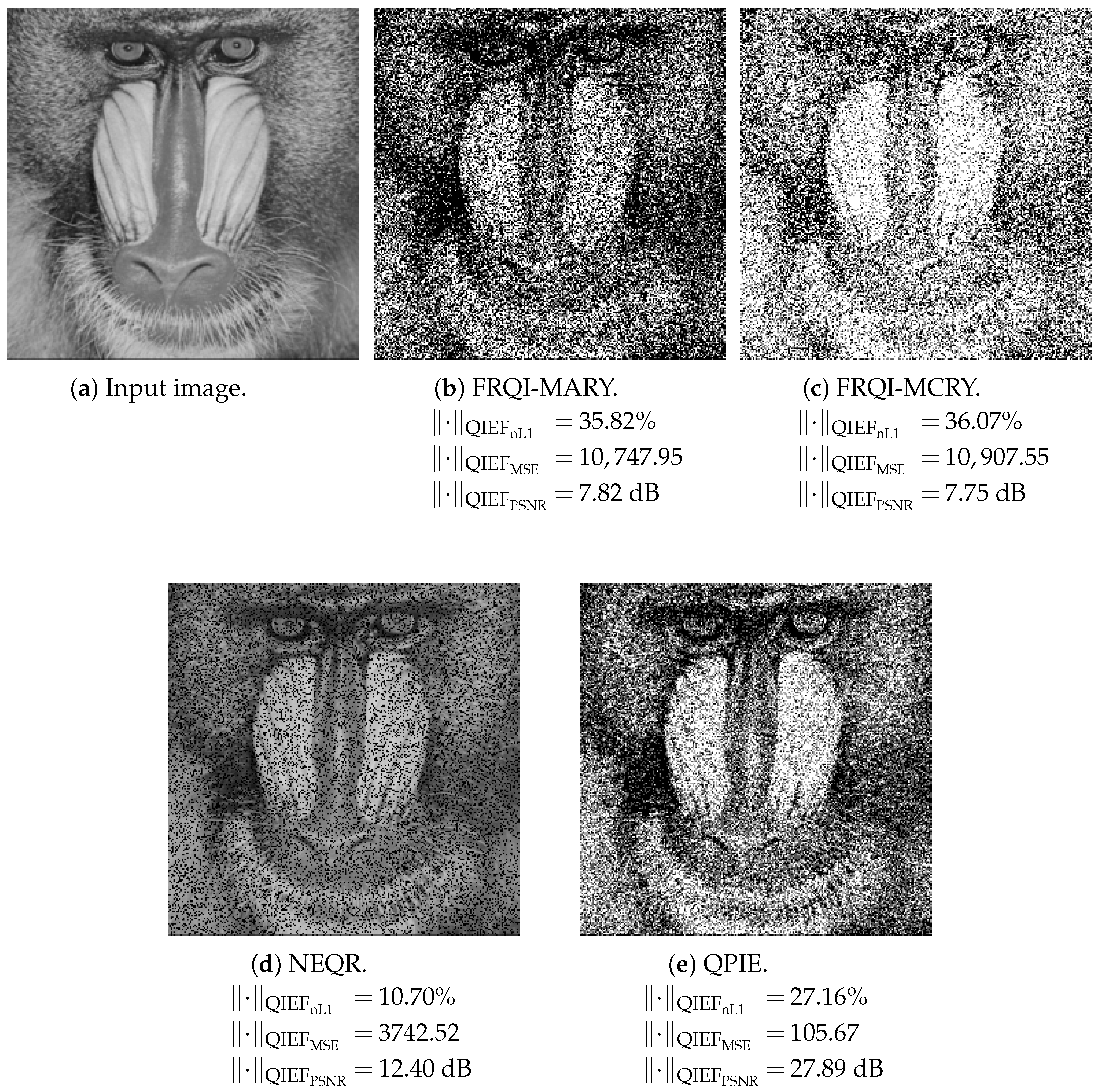
Figure 7 shows the visual results of the $256\times 256$ sample image together with the quantum image encoding fidelity metric values ${\parallel ·\parallel }_{{\mathrm{QIEF}}_{\mathrm{nL}1}},{\parallel ·\parallel }_{{\mathrm{QIEF}}_{\mathrm{MSE}}},{\parallel ·\parallel }_{{\mathrm{QIEF}}_{\mathrm{PSNR}}}$ and the required execution times needed to calculate the results.

When comparing the quantum image encoding methods, we observe that the NEQR method yields slightly better reconstruction results than the QPIE method. This can be attributed primarily to the nature of image retrieval following measurement. In NEQR, the goal is to identify the quantum state with the highest probability at each pixel position, which allows for deterministic image reconstruction. As a result, the exact probability values are not critical. In contrast, QPIE stores pixel values in the amplitudes of the quantum state, requiring reconstruction based on sampled probabilities. Typically, the median amplitude is used for this purpose (see [20]), which also explains the normalized appearance of the reconstructed images.

For both variants of the FRQI method, image reconstruction involves combining measurement outcomes from the gray-value qubit in both $|0\rangle$ and $|1\rangle$ states for each pixel position (see Equation (6)). Because the gray value is inferred from the relative frequencies of these two outcomes, even slight noise-induced deviations in one of the probabilities can lead to noticeable inaccuracies in the final pixel intensity. This makes FRQI-based methods more sensitive to noise compared to NEQR’s deterministic approach.

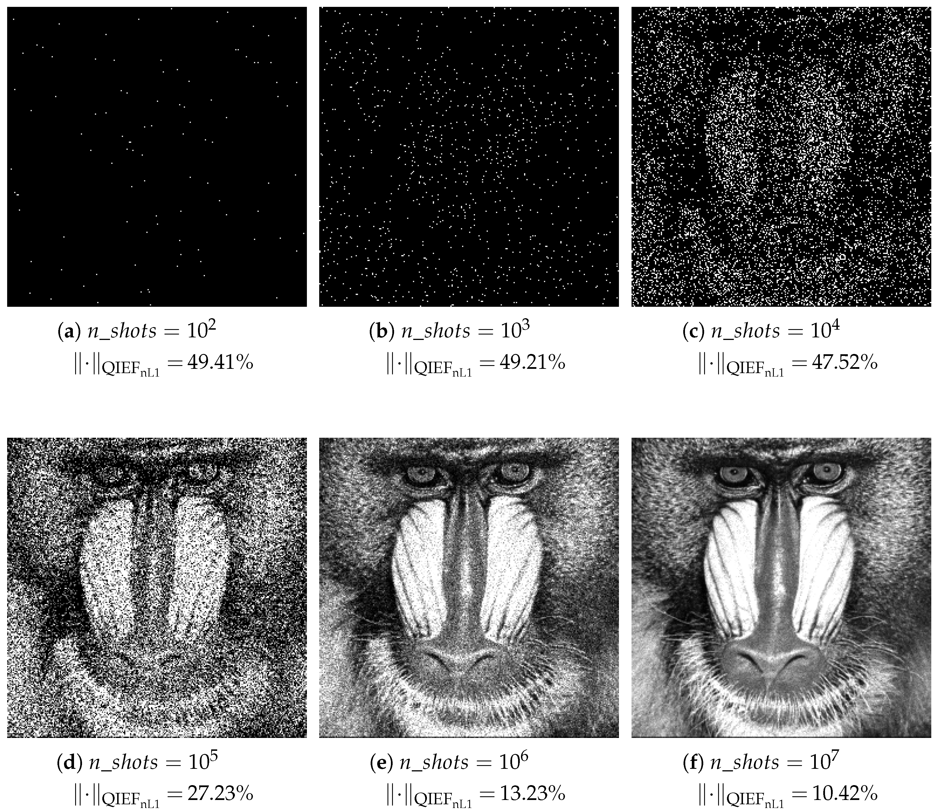
As illustrated in Figure 7, the reconstruction quality on the qasm_simulator but also on other simulators or real devices, is highly sensitive to the number of shots used during execution. To systematically examine this effect, we selected the Quantum Probability Image Encoding (QPIE) method and varied the number of shots as $n\_shots\in \{{10}^2,{10}^3,\dots ,{10}^7\}$. The results, shown in Figure 8, reveal that for $n\_shots\le {10}^4$, the reconstructed image of the baboon is largely unrecognizable. This visual degradation is also quantitatively confirmed by high quantum image encoding fidelity values, with ${\parallel ·\parallel }_{{\mathrm{QIEF}}_{\mathrm{nL}1}}$ exceeding $47\%$. From $n\_shots={10}^4$ onward, the structural features of the baboon become clearly visible, accompanied by a corresponding decrease in the fidelity metric. In this experiment it is also visible that the quantum image encoding fidelity metric can be used as an application-based metric.

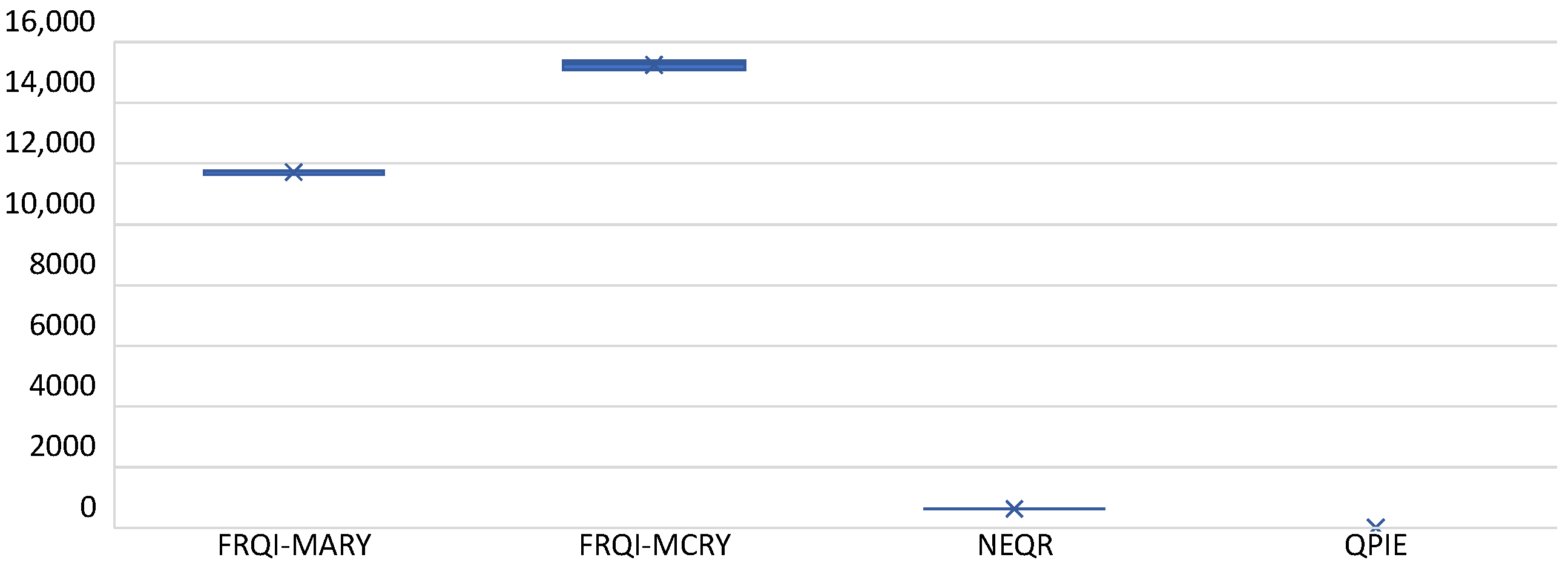
A comparison of execution times in Figure 9 reveals significant differences among the NEQR, QPIE, and the two FRQI variants. On average, the execution times for the different encoding methods are as follows: approximately $0.53$ s for QPIE, $624.50$ s for NEQR, $11,720.40$ s for FRQI-MARY, and $15,253.40$ s for FRQI-MCRY. These values reflect the substantial variation in circuit complexity and circuit depth across the encoding strategies, particularly on real quantum hardware where decomposition into native gate sets significantly impacts performance. These differences arise primarily from the distinct encoding strategies and their respective circuit complexities, especially under noise and hardware limitations. The FRQI-MCRY method employs a custom multi-controlled rotation gate, which is tailored for quantum execution but introduces substantial circuit depth. In contrast, FRQI-MARY is explicitly designed to reduce the number of two-qubit gates of the FRQI-MCRY method, thereby reducing the source of noise and improving performance/speed on NISQ devices (see [20]).

NEQR and particularly QPIE exhibit notably shorter execution times when implemented using the Qiskit built-in function circ.initialize(state) on qasm_simulator. This approach is advantageous in simulation, as the full state vector is initialized directly, bypassing the need for gate-by-gate construction. However, such high-level initializations must be decomposed into the native gate set of the specific backend on real quantum hardware, too.

What Is Needed to Run the Experiments on the Real Hardware?

The experiments conducted on the $256\times 256$ Mandrill (Baboon) image, as previously discussed, were executed directly on the qasm_simulator without transforming the quantum circuits into hardware-specific basis gates. 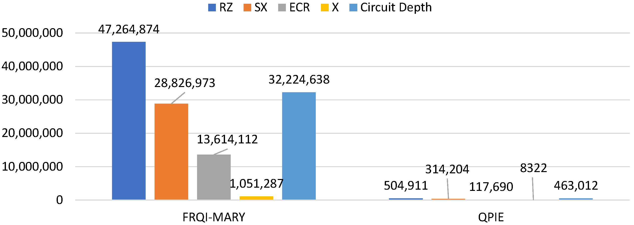To better understand current hardware limitations, we additionally transpiled the quantum circuits using backend-specific constraints, such as those of ibm_sherbrooke, by invoking transpile(circuit, backend=ibm_sherbrooke). This transpilation process converts high-level quantum gates into a sequence of native basis gates—specifically RZ, SX, ECR, and X—supported by the target device. From the transpiled circuits, we extracted both the circuit depth and the number of required basis gates. The results are visualized in Figure 10, which presents the basis gate counts and circuit depths for the three $256\times 256$ sample images. These values provide insight into the scalability challenges and execution feasibility of large-scale quantum image encoding on real quantum hardware.

8.3. Interpretation of Gate Counts and Circuit Depth

The FRQI-MARY method results in an extremely large number of basis gates, with over 46 million RZ gates, 28 million SX gates, and over 13 million ECR gates. Its circuit depth also exceeds 28 million. These values highlight the considerable complexity of the FRQI-MARY circuits when mapped to the native gate set of current superconducting quantum devices, making practical execution on real hardware currently infeasible.

In contrast, the QPIE method demonstrates significantly lower resource requirements. The total gate counts remain below 1 million for each gate type, and the circuit depth is around 500,000. This huge difference comes from QPIE’s implementation using circ.initialize(state), which, although not hardware-executable in its raw form, simplifies simulation and reduces logical depth before transpilation. However, real hardware would still require this initialization to be decomposed into basis gates, potentially increasing the practical gate counts.

Overall, this comparison highlights the scalability challenges of phase-encoded methods like FRQI-MCRY and FRQI-MARY on current quantum devices, while also showcasing the relative efficiency of amplitude-based methods such as QPIE—at least in simulation or theoretical circuit design. These results reinforce the importance of transpilation-aware analysis when evaluating the feasibility of quantum algorithms on actual hardware backends.

In the case of NEQR, the encoding inherently requires multi-controlled operations between the position qubits and the color qubits. For the $256\times 256$ image samples used in our experiments, this translates to 16 position qubits (to address all $65,536$ pixel locations) and 8 color qubits (for representing gray-level intensity values in the range $[0,255]$). As previously demonstrated in [20] using a $2\times 2$ example, the NEQR method necessitates entangling all position qubits with each individual color qubit via multi-controlled MCX gates. This operation must be repeated for each color qubit, resulting in a highly complex and deep quantum circuit.

Transpiling such large multi-controlled gates into basis gates imposes a significant computational burden. In practice, this often leads to memory exhaustion during transpilation, especially for large image sizes. Subsequently, the execution of this circuits on current quantum hardware is unattainable to obtain reliable circuit depth or gate count values for the NEQR method, and thus these are omitted from Figure 10.

These observations emphasize the critical role of hardware-aware circuit design and application-based metrics and provide context for the observed variation in performance across encoding methods.

9. Conclusions and Discussion

In this work, we introduced the Quantum Image Encoding Fidelity (QIEF) as a task-specific metric to evaluate the performance of quantum devices and algorithms in the context of image processing. Unlike general-purpose hardware benchmarks such as gate fidelity or quantum volume, QIEF directly reflects how well a quantum system preserves image information through the encoding, execution, and decoding pipeline. Through comprehensive experiments on both simulators and real quantum hardware, we demonstrated that QIEF can effectively distinguish between the capabilities of various quantum technologies and encoding methods.

Our results indicate that image encoding techniques such as NEQR and QBIP yield perfect reconstructions under ideal conditions, whereas amplitude and phase-based encodings are more susceptible to noise and measurement ambiguity. The comparative analysis of quantum simulators and real devices highlighted the critical influence of hardware noise, limited coherence times, and qubit connectivity on image fidelity. Notably, we observed that QIEF can sensitively detect such performance bottlenecks, making it a practical and insightful tool for application-level benchmarking.

Beyond its use as an evaluation metric, QIEF offers significant extensibility for integration with more complex quantum tasks. For instance, in quantum image segmentation, QIEF can serve not only as a fidelity metric for the encoded input but also for the segmented output. By incorporating segmentation algorithms—classical or quantum—into the QIEF evaluation schema, we can measure the end-to-end performance of hybrid quantum–classical workflows. Furthermore, QIEF could be used within optimization loops, such as in quantum variational circuits or during training of quantum neural networks, to directly guide learning based on image reconstruction fidelity.

As quantum hardware continues to evolve, the ability to assess its usefulness in domain-specific tasks will become increasingly important. The QIEF metric provides a foundational step toward that goal, offering a structured and interpretable way to quantify image-related quantum processing performance. Future work could explore extending QIEF to color images, video frames, or three-dimensional data and integrating it with other perceptual similarity metrics to further refine its sensitivity and robustness.

In conclusion, QIEF bridges the gap between abstract quantum performance metrics and real-world application requirements, thereby facilitating a more meaningful and visually intuitive comparison of quantum computing platforms in image processing domains. This task-aware approach to benchmarking opens new avenues for research and practical deployment of quantum image processing algorithms.