Electric Power Consumption Forecasting in Bulgaria ^†

Abstract

The primary goal of this paper is to develop a robust model for forecasting electric power consumption in Bulgaria. Leveraging historical forecast data from Open-Meteo for weather-related features and ENTSOE data, our objective is to create an accurate prediction tool that can assist in optimizing energy management within the country. By achieving this goal, we aim to improve energy reliability, support data-driven decision making in energy policy, and promote sustainable energy practices in Bulgaria. This predictive model will empower us to proactively address fluctuations in energy demand, particularly during extreme weather conditions, and will contribute to the efficient allocation of electrical resources.

1. Introduction

Accurate electricity load forecasting is essential for the reliable and efficient operation of modern power systems. It underpins key processes such as generation scheduling, grid balancing, and infrastructure planning while also reducing operational costs and uncertainty. In liberalized electricity markets, forecasting plays a central role in supporting participation in organized trading environments, particularly in the day-ahead market, where electricity is traded through a centralized bidding and clearing mechanism that determines hourly schedules [1].

Traditional approaches to load forecasting have relied on statistical time-series models such as Seasonal Autoregressive Integrated Moving Average (SARIMA) and exponential smoothing. While these methods are valued [2] for their interpretability and solid theoretical foundation, they often fail to capture the nonlinear dependencies [3] and complex interactions between demand and exogenous variables observed in modern energy systems. To address these limitations, recent research has increasingly adopted machine learning techniques, including Random Forest, XGBoost, LightGBM, and neural networks. These models are capable of extracting complex nonlinear patterns from high-dimensional datasets and have demonstrated improved forecasting accuracy, particularly in settings where multiple external drivers influence consumption.

However, the performance of such models critically depends on the appropriate incorporation of regional and exogenous factors [4]. Weather and calendar variables—such as temperature variations, wind conditions, and public holidays—are among the most significant determinants of electricity demand. In the context of the Bulgarian power system, capturing these localized dynamics is essential for achieving reliable and precise forecasts [5].

Despite the significant progress achieved by recent machine learning approaches, several limitations remain. Existing studies often rely on highly complex hybrid architectures that are computationally intensive and difficult to interpret [5,6,7], limiting their practical applicability in real-world power system operations. Furthermore, there is a lack of consistency in data preprocessing, feature selection, and evaluation methodologies, which complicates the comparison of results across different studies. Importantly, many models are developed for specific regional markets and do not explicitly address the challenges associated with adapting forecasting frameworks to localized system characteristics. These limitations highlight the need for robust, scalable, and regionally adaptable forecasting approaches.

In this paper, a supervised machine learning framework is developed to forecast the hourly total electricity load in Bulgaria. The proposed approach leverages gradient boosting techniques combined with carefully engineered weather-based features to capture the underlying demand patterns. The following sections present the data sources, feature engineering procedures, and methodological framework used in the analysis.

2. Materials and Methods

2.1. Recent Advances in Electrcity Load Forecasting

We begin with a comparative overview of recent machine learning approaches for electricity load forecasting, as summarized in

Table 1. Summary of ML models for load forecasting.

Reference	Publication	Model	Sample Size	Train/Test/Val Set	Feat.	Error Metrics
[5] Wang B. et al.	2025	CEEMDAN-CNN-BiLSTM	25 days	25:1:0	5	RMSE = 154.21 MW, $R^2$ = 0.983, MAE = 117.47 MW, MAPE = 1.396%
[6] Ning Z. et al.	2025	TKNFD-Transformer	15 years	12:3:0	38–92	MAPE ≈ 1.4%
[7] Ullah K. et al.	2024	CNN-LSTM	53 months	34:15:5	10	RMSE = 951.94, MAE = 656.35, MAPE = 4.72%
[8] Abbas M. et al.	2025	AdaBoost-LGB-MLP-KAN	5 years	4:1:0	21	MAPE = 2.05%, RMSE = 353.52 MW, MAE = 289.96 MW
[9] Zhao Q. et al.	2025	TPE-XGB-CS-BiLSTM	3 years	1:1:1	286	MAE = 27.77 MW, RMSE = 40.45 MW, MAPE = 2.98%, $R^2$ = 94.06
[10] Karamolegkos S. et al.	2025	FARIMA	10 years	51:1:0	3	MAPE = 7.96%, RMSE = 813.98, MSE = 662,556.46
[11] Liu M. et al.	2025	iMICN	5 years	8:1:1	7	MAPE = 0.41%, MAE = 62.12 MW, RMSE = 202.23 MW
[12] Zhao J. et al.	2024	LASTGCN	16 months	7:2:1	31	MAE = 0.0246 MWh, RMSE = 0.0455, $R^2$ = 0.7991
[13] Xu F. et al.	2024	VMD-Nyström-BiTCN	1 year	50:3:0	1	MAE = 8.35, SAE = 0.042
[14] Gong J. et al.	2025	TCN-LSTM-LGB	5 years	6:2:2	7	MAPE = 0.519%, MAE = 46.1 MW, RMSE = 62.3 MW
[15] Aguilar Madrid E.; Antonio N.	2021	XGB	65 months	51:14:0	13	MAPE = 3.74%, RMSE = 55.6 MW
[16] Timur O.; Üstünel H.Y.	2025	GB	3 years	80:20:0	13	MAPE = 0.827%, RMSE = 55.6 MW
This Paper	2026	LightGBM	2 years	1:1:1	31	MAPE = 2.56%, MAE = 108.60 MW

. The table compiles a selection of contemporary studies, highlighting the diversity of modeling techniques, dataset sizes, feature configurations, and evaluation metrics used in the literature. In addition to model architectures, particular attention is given to the data-splitting strategies and the scale of input features, both of which significantly influence reported performance. This overview provides the necessary context for positioning the proposed methodology within the current state of research.

As shown in Table 1, recent advances in load forecasting are dominated by hybrid and deep learning architectures, often combining decomposition techniques, neural networks, and gradient boosting methods. These approaches generally achieve lower forecasting errors compared to traditional statistical models, although their performance varies significantly depending on dataset size and feature richness.

A key limitation observed across the literature is the lack of standardization. Sample sizes range from a few weeks to over a decade, while feature sets vary from a single variable to several hundred inputs. In addition, different train–test–validation splits are employed, making a direct comparison of performance metrics such as MAPE, MAE, and RMSE inherently difficult.

Despite this heterogeneity, a consistent trend emerges: models incorporating exogenous variables and hybrid structures tend to achieve superior predictive accuracy. However, these gains are often accompanied by increased model complexity and reduced interpretability.

In this context, this paper adopts a gradient boosting framework, aiming to balance predictive accuracy and model efficiency while using a feature set tailored to the characteristics of the Bulgarian power system.

The accuracy of the models in Table 1 are mainly validated using the following formulas:

• Mean absolute error (MAE) is given by

  $$MAE={\displaystyle \frac{1}{n}}{\displaystyle \sum _{i=1}^n}|y_i-{\widehat{y}}_i|$$
• Root mean square error (RMSE) is given by

  $$RMSE=\sqrt{{\displaystyle \frac{1}{n}}\sum _{i=1}^n{(y_i-{\widehat{y}}_i)}^2}$$
• Mean absolute percentage error (MAPE) is given by

  $$MAPE={\displaystyle \frac{100\%}{n}}{\displaystyle \sum _{i=1}^n}\left|{\displaystyle \frac{y_i-{\widehat{y}}_i}{y_i}}\right|$$
• Mean squared error (MSE) is given by

  $$MSE={\displaystyle \frac{1}{n}}{\displaystyle \sum _{i=1}^n}{(y_i-{\widehat{y}}_i)}^2$$

Despite their utility, these statistical metrics lack a temporal dimension, failing to distinguish between errors occurring during critical peak hours versus those during low-demand periods. Furthermore, they do not account for the sign of the error, which is an important omission for system operators who view under-prediction (leading to shortages) as far more hazardous than over-prediction. By monitoring this collective set, we achieve a robust validation framework that addresses both economic efficiency and operational security. It is worth mentioning, however, they do not tell us where exactly the error is: if we systematically under-predict or over-predict weekdays vs. the weekend, holidays vs. normal days, or specific hours.

The proliferation of bespoke hybrid architectures, often plagued by a lack of reproducibility when applied to external datasets, highlights a significant limitation in their scalability across diverse power systems. Because these hybrid models are frequently over-optimized for the specific characteristics of their training data, they often fail to function as universal forecasting solutions. In contrast, standalone Machine Learning (ML) and Deep Learning (DL) frameworks offer greater scalability. As illustrated in Table 1, the current research landscape is dominated by DL architectures such as LSTM, CNN, TCN, and RNN—a trend also corroborated by Zhao J. et al. [14]. However, our synthesis of the existing literature suggests that standalone DL models rarely achieve the highest accuracy on their own.

Interestingly, traditional ML models maintain significant relevance; despite their lower computational complexity, they continue to deliver highly competitive results. Notably, in 2 out of the 11 publications reviewed, basic models (such as GB and XGB) and ensemble techniques (including Random Forest, XGBoost, and AdaBoost) actually outperformed more complex hybrid and DL counterparts. Among these, the most precise results in terms of MAPE were achieved by XGBoost (3.74%) [7] and Gradient Boosting (0.827%) in [16], suggesting that architectural simplicity combined with robust feature engineering remains a formidable approach in the field.

The use of real meteorological data in the papers is also very misleading because in reality, where predictions are made from day to day, forecast data is used rather than actual data. Therefore, the error from the weather provider should be accounted for in the training, whereas often in papers, it is not even mentioned. Our understanding is that most researchers tend to try hybrid models in order to try and explain with higher mathematical complexity the electricity consumption. In our opinion, this is a wrong approach. The emphasis should be put on the quality of the exogenous variables and the weights of each one rather than the calibration of the models for a particular dataset, as it is prone to overfit.

2.2. Data Collection/Sources

The historical electricity consumption data for Bulgaria are retrieved from the European Network of Transmission System Operators for Electricity (ENTSO-E) Transparency Platform. As of 2026, ENTSOE serves as the central data hub for 36 member countries, where each national Transmission System Operator (TSO)—in this case, Bulgaria’s ESO (Electroenergien Sistemen Operator)—is legally mandated to report real-time and historical power statistics.We utilize the Actual Total Load parameter, which represents the hourly average of the total electricity consumed within the Bulgarian bidding zone. The use of ENTSO-E data ensures a high degree of accuracy and cross-border consistency, as the platform employs rigorous validation protocols to harmonize reporting from different national authorities. For our forecasting pipeline, these data are available with a $T-24$ latency, meaning the previous day’s complete hourly profile is accessible for next-day scheduling.

The availability, temporal resolution, and sources of the input features and exogenous variables used in this study are summarized in

Table 2. Data availability.

Features and Exogenous Variables	Source	Temporal Resolution, h	Availability
Volume Y, M, D, H	The dataset itself Datetime library	1	$X-1$ Anytime
Meteorological data	https://open-meteo.com/en/docs/historical-forecast-api (accessed on 1 May 2026)	1	$X+2$ weeks ahead
Electricity consumption (actual total load)	https://www.entsoe.eu/data/power-stats/ (accessed on 1 May 2026)	1	$T-24$ Available from previous day
lag-1 …lag-7	The dataset itself	1	$X-2$

.

To account for the high sensitivity of electricity demand to weather conditions, we incorporate meteorological data from the Open-Meteo Historical Forecast API. Open-Meteo is an open-source weather API that aggregates data from global national weather services, such as the ECMWF (European Centre for Medium-Range Weather Forecasts) and NOAA (National Oceanic and Atmospheric Administration). Unlike standard historical weather stations, Open-Meteo provides reanalysis data and historical forecasts, which are essential for supervised learning. This allows our model to be trained not just on what the weather was but also on the weather forecasts that were available at the time of the prediction. This better simulates real-world operational constraints. The API provides hourly resolution for variables such as temperature at 2 m, wind speed, solar radiation and many more with a forecasting horizon extending up to two weeks ($X+14$ days), allowing for both short-term and mid-term load projections.

To represent climatic conditions across the country, weather data were extracted for four major Bulgarian cities—Sofia, Plovdiv, Varna, and Ruse—which serve as geographical proxies for the main consumption hubs. We then calculated the arithmetic mean for each meteorological feature across these locations to create a single, representative national weather profile for the forecasting model.

In the next subsection, we will explain more in detail how to create from the internal dataset calendar features and reduce dimensions by combining data from different locations.

2.3. Feature Creation/Calendar Features

The inclusion of calendar-based explanatory variables was motivated by the temporal nature of electricity demand, which is strongly influenced by recurring behavioral, climatic, and structural patterns. Since electricity consumption is not random through time, incorporating variables derived from the timestamp allows the model to capture systematic variations that would otherwise remain unexplained.

The year variable was introduced to account for long-term structural changes in demand. Over multiple years, electricity consumption may evolve due to economic growth, demographic changes, improvements in energy efficiency, the electrification of transport and heating, or changes in industrial activity. Including the year feature allows the model to represent gradual shifts in baseline demand across the sample period.

The quarter variable was included to capture broad seasonal regimes within the year. Electricity demand often differs substantially between winter, spring, summer, and autumn due to heating and cooling requirements, daylight duration, and changes in economic activity. Grouping the year into quarters provides a parsimonious way to model these wider seasonal transitions.

The month variable was used to capture finer seasonal effects that cannot be fully represented by quarters alone. For example, January demand may differ considerably from March despite both belonging to the same broad seasonal period. Monthly effects may also reflect holiday seasons, tourism cycles, and transitional weather conditions.

The week variable was incorporated to represent medium-term cyclical patterns throughout the year. Weekly indexing can capture evolving demand conditions such as school terms, vacation periods, public activity cycles, and gradual seasonal transitions that occur more smoothly than monthly categories.

The day of year variable was included to model the continuous annual cycle of demand. Unlike month or quarter, which impose discrete boundaries, day of year allows the model to learn gradual seasonal progression across the calendar year. This is particularly useful when demand changes smoothly as temperatures rise or fall over time.

The day of week variable was introduced because electricity usage patterns differ systematically across weekdays. Commercial and industrial activity is typically higher during working days, while household behavior changes on weekends. As a result, Monday demand profiles often differ from those observed on Saturday or Sunday.

The hour variable was included to capture intraday seasonality, which is one of the strongest drivers of hourly electricity demand. Load usually follows predictable daily cycles shaped by waking hours, working schedules, meal preparation, lighting needs, and overnight reductions in activity. Morning and evening peaks are commonly observed in many power systems [17].

The weekend indicator was created as a simplified binary representation of behavioral differences between working days and non-working days. While day of week provides detailed categorical information, the weekend variable offers a more direct distinction between business-oriented and leisure-oriented demand patterns.

The holiday indicator was included because public holidays often generate atypical consumption behaviour. Commercial demand may decline due to business closures, while residential demand may increase as more people remain at home. Holiday effects frequently resemble weekends but may also exhibit unique characteristics depending on the specific holiday and season [17].

These model feature creation approaches are explored and demonstrated in [18,19]. From there heat map, cluster and correlations on similar datasets can be found.

Overall, these calendar variables were selected because they reflect economically and behaviorally meaningful sources of variation in electricity demand. Their inclusion improves the model’s ability to capture recurring temporal structures, enhances forecasting accuracy, and reduces the burden on the algorithm to infer such patterns solely from lagged observations.

This finalizes all of the features.

Temperature	Humidity / Moisture	Precipitation
temperature_2m (°C), dew_point_2m (°C), apparent_temperature (°C), temperature_80m (°C), temperature_120m (°C), temperature_180m (°C), soil_temperature_0cm (°C), soil_temperature_6cm (°C), soil_temperature_18cm (°C), soil_temperature_54cm (°C), wet_bulb_temperature_2m (°C)	relative_humidity_2m (%), vapour_pressure_deficit (kPa), soil_moisture_0_to_1cm (m3/m3), soil_moisture_1_to_3cm (m3/m3), soil_moisture_3_to_9cm (m3/m3), soil_moisture_9_to_27cm (m3/m3), soil_moisture_27_to_81cm (m3/m3)	precipitation (mm), rain (mm), showers (mm), snowfall (cm), snow_depth (m), precipitation_probability (%)
Pressure / Radiation	Cloud / Visibility	Wind
pressure_msl (hPa), surface_pressure (hPa), shortwave_radiation (W/m2), direct_radiation (W/m2), diffuse_radiation (W/m2), direct_normal_irradiance (W/m2), global_tilted_irradiance (W/m2), terrestrial_radiation (W/m2), evapotranspiration (mm), et0_fao_evapotranspiration (mm)	cloud_cover (%), cloud_cover_low (%), cloud_cover_mid (%), cloud_cover_high (%), visibility (m), sunshine_duration (s)	wind_speed_10m (km/h), wind_speed_80m (km/h), wind_speed_120m (km/h), wind_speed_180m (km/h), wind_direction_10m (°), wind_direction_80m (°), wind_direction_120m (°), wind_direction_180m (°), wind_gusts_10m (km/h)
UV / Daylight	Calendar Features
uv_index, uv_index_clear_sky, is_day	year, quarter, dayofweek, hour, is_holiday, is_weekend

Next, we will explore the mathematical meaning behind gradient boosting to obtain an idea how the model accepts all these data and why this is important to use.

2.4. Mathematics of Gradient Boosting and LightGBM

Gradient boosting and LightGBM can be understood as methods for solving a functional optimization problem over a space of measurable functions.

Let $(\mathcal{X},\mathcal{A})$ be a measurable input space, typically $\mathcal{X}\subseteq {\mathbb{R}}^d$, and let $\mathcal{Y}\subseteq \mathbb{R}$ be the output space. We are given a dataset

$${\left\{(x_i,y_i)\right\}}_{i=1}^n\subset \mathcal{X}\times \mathcal{Y},$$

(1)

drawn i.i.d. from an unknown probability measure P.

We consider a hypothesis space $\mathcal{F}$ of measurable functions

$$f:\mathcal{X}\to \mathbb{R}.$$

(2)

Let $L:\mathcal{Y}\times \mathbb{R}\to {\mathbb{R}}_{+}$ be a loss function. The associated risk functional is

$$\mathcal{R}\left(f\right)={\mathbb{E}}_{(x,y)\sim P}\left[L(y, f(x\left)\right)\right],$$

(3)

with empirical counterpart

$${\mathcal{R}}_n\left(f\right)={\displaystyle \frac{1}{n}}{\displaystyle \sum _{i=1}^n}L(y_i, f(x_i\left)\right).$$

(4)

A loss-induced discrepancy between functions can be defined as

$$d_L(f, g)=\mathbb{E}\left[\left|L\right(y, f\left(x\right))-L(y, g\left(x\right)\left)\right|\right].$$

(5)

For squared loss, this corresponds to an $L^2\left(P\right)$-type structure.

Gradient boosting constructs an additive model of the form

$$f_M\left(x\right)={\displaystyle \sum _{m=1}^M}{\gamma }_m{h}_m\left(x\right),$$

(6)

where $h_m\in \mathcal{H}$ is a regression tree. The associated function class is

$${\mathcal{F}}_M=\left\{{\displaystyle \sum _{m=1}^M}{\gamma }_m{h}_m:h_m\in \mathcal{H},{\gamma }_m\in \mathbb{R}\right\}.$$

(7)

The learning problem is

$$\underset{f\in {\mathcal{F}}_M}{\min }{\mathcal{R}}_n\left(f\right).$$

(8)

This is solved via functional gradient descent:

$$f_m=f_{m-1}+{\gamma }_m{h}_m,$$

(9)

where $h_m$ approximates the negative gradient of the empirical risk.

The functional derivative is

$${\displaystyle \frac{\delta {\mathcal{R}}_n}{\delta f}}\left(x_i\right)={\displaystyle \frac{\partial L(y_i, f(x_i\left)\right)}{\partial f\left(x_i\right)}}.$$

(10)

The pseudo-residuals are defined as

$$r_i^{\left(m\right)}=-{\left.{\displaystyle \frac{\partial L(y_i, f(x_i\left)\right)}{\partial f\left(x_i\right)}}\right|}_{f=f_{m-1}}.$$

(11)

The next base learner is obtained by

$$h_m=\arg \underset{h\in \mathcal{H}}{\min }{\displaystyle \sum _{i=1}^n}{\left(r_i^{\left(m\right)}-h\left(x_i\right)\right)}^2.$$

(12)

This can be interpreted as a greedy projection of the negative gradient onto the space of regression trees.

Second-Order Boosting (LightGBM)

LightGBM incorporates second-order information. A Taylor expansion gives

$$L(y_i, f(x_i)+h(x_i\left)\right)\approx L(y_i, f(x_i\left)\right)+g_{i}h(x_i)+{\displaystyle \frac{1}{2}}{h}_{i}h{\left(x_i\right)}^2,$$

(13)

where

$$g_i={\displaystyle \frac{\partial L(y_i, f(x_i\left)\right)}{\partial f\left(x_i\right)}},h_i={\displaystyle \frac{{\partial }^{2}L(y_i, f(x_i\left)\right)}{\partial f{\left(x_i\right)}^2}}.$$

(14)

The corresponding objective becomes

$${\mathcal{L}}^{\left(m\right)}={\displaystyle \sum _{i=1}^n}\left(g_{i}h(x_i)+{\displaystyle \frac{1}{2}}{h}_{i}h{\left(x_i\right)}^2\right).$$

(15)

Each tree has the form

$$h\left(x\right)=w_{q\left(x\right)},$$

(16)

where $q\left(x\right)$ maps inputs to leaf indices.

The regularized objective is

$$\mathcal{L}\left(f\right)={\displaystyle \sum _{i=1}^n}L(y_i, f(x_i\left)\right)+{\displaystyle \sum _{m=1}^M}\mathsf{\Omega }(h_m),$$

(17)

with

$$\mathsf{\Omega }(h)=\gamma T+{\displaystyle \frac{1}{2}}\lambda {\displaystyle \sum _{j=1}^T}{w}_j^2.$$

(18)

For a fixed tree structure, optimal leaf weights are

$$w_j=-{\displaystyle \frac{{\sum }_{i\in I_j}{g}_i}{{\sum }_{i\in I_j}{h}_i+\lambda }}.$$

(19)

In the next subsection, we construct a Python 3.11 implementation based on this formulation.

2.5. Model-Feature Selection and Validation Process

Model selection can be completed in many ways, depending on the dataset.

2.5.1. Model Selection

Several forecasting strategies exist for multi-step time-series prediction, including recursive autoregressive forecasting, direct multi-step forecasting, and multiple-output forecasting.

In the recursive autoregressive approach, a one-step-ahead model is first estimated and then repeatedly applied to generate forecasts further into the future. For example, the prediction for period $t+2$ uses the forecasted value from period $t+1$ as an input. While computationally efficient, this method suffers from error accumulation, since mistakes made in earlier steps propagate into later forecasts.

In the direct multi-step forecasting approach, a separate model is estimated for each forecast horizon. Thus, one model predicts $t+1$, another predicts $t+2$, and so forth. Each forecast is generated directly from observed historical information rather than previous predictions.

A third alternative is multiple-output forecasting, where a single model simultaneously predicts several future horizons in one step. Although this can capture dependencies across horizons, it often requires more complex model structures and greater computational effort.

The direct multi-step approach was preferred for several reasons. First, it avoids the error propagation problem present in recursive forecasting, since later forecasts do not depend on earlier predicted values. Second, each horizon can learn its own dynamics, which is valuable when short-term and longer-term demand patterns differ. Third, it is well suited to electricity load forecasting, where the determinants of one-hour-ahead demand may differ from those affecting demand one day ahead. Therefore, the direct multi-step framework offers greater robustness and flexibility, making it particularly suitable for multi-horizon electricity demand forecasting.

2.5.2. Validation Method

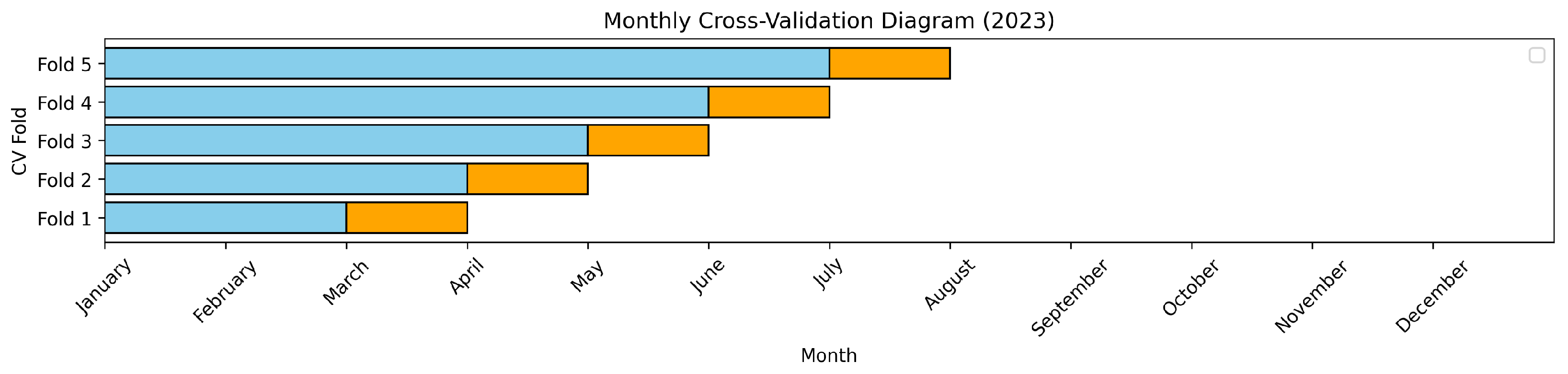
The least amount of train data we need is 1 year. For this purpose, we will use the dataset for 2023 to data train and test. The reason is that, as we established, the electricity demand is cyclical and the largest cycle is per season. Meaning, our model must see all seasons (spring, summer, autumn, winter) to cover the calendar features and the seasonal cycles. For this, we need to split the data into train/test. Then, we will make use of a technique called cross-validation. Cross-validation is best seen with CV-folds set to 12, as there are 12 months in the year, and a minimization function on MAE, as illustrated in Figure 1.

After running the sklearn.model_selection cross-validation with MAE as the evaluation metric, the following results were obtained, as shown in

Table 3. Performance comparison of candidate models (all features).

Model	Description/Configuration	MAE (MW)
Random Forest	Ensemble of decision trees using bagging and feature randomness to reduce variance.	298.70
AdaBoost	Adaptive boosting that weights misclassified instances from previous weak learners.	414.37
LightGBM	Gradient boosting framework using leaf-wise growth and histogram-based decision trees for high efficiency.	298.36
XGBoost	Scalable end-to-end tree boosting system using second-order Taylor expansion for the loss function.	310.35

Note: Bold indicates the best-performing model based on the lowest mean absolute error (MAE).

.

Cross-validation was used because a single train–test split can give an unreliable estimate of model performance. The results may depend heavily on the observations that are randomly assigned to the training or testing sets. Cross-validation reduces this randomness by evaluating the model in multiple data partitions.

In K-fold cross-validation, the dataset is divided into K subsets. The model is trained on $K-1$ folds and validated on the remaining fold. This process is repeated until each fold has been used once for validation, and the average error is calculated:

$$CV={\displaystyle \frac{1}{K}}{\displaystyle \sum _{k=1}^K}{L}_k$$

where $L_k$ is the validation loss in fold k.

This approach was adopted for several reasons.

First, it provides a more robust estimate of out-of-sample predictive accuracy than a single split. Second, it helps detect overfitting, as models that perform well only on training data tend to show weaker validation results. Third, it uses the dataset more efficiently, since each observation is used for both training and validation across different folds. Fourth, it enables fair comparison between competing models and supports hyperparameter tuning.

For electricity demand forecasting, where data contain seasonality and changing patterns over time, cross-validation provides a more credible basis for model selection. It therefore improves confidence that the selected model will generalize well to unseen observations.

3. Discussion

We start by selecting the type of forecasting method we use—direct multi-step forecasting, as explained in the previous section. Next, we use cross-validation on 12 months to select the features. For this, we run Optuna, which is a python open source library with a brute force of 200 trials and early stopping, producing the following best features on the 2023 data.

The selected features obtained through the 12-fold cross-validation feature selection procedure are presented in

Table 4. Selected features obtained via 12-fold cross-validation feature selection.

Category	Selected Features
Atmospheric Variables	relative_humidity_2m, dew_point_2m, wet_bulb_temperature_2m, visibility
Precipitation Variables	precipitation, precipitation_probability, rain, showers
Wind Variables	wind_speed_10m, wind_gusts_10m, wind_direction_120m, wind_direction_180m
Temperature Variables	temperature_120m, temperature_180m, soil_temperature_0cm, soil_temperature_18cm, soil_temperature_54cm
Radiation Variables	shortwave_radiation, diffuse_radiation, global_tilted_irradiance, terrestrial_radiation, sunshine_duration, uv_index, uv_index_clear_sky
Soil Variables	soil_moisture_3_to_9cm, evapotranspiration
Temporal Features	week, dayofweek, hour, is_weekend, is_holiday

.

The above hyperparameters were obtained using Optuna through a brute-force style search over 200 trials. Each trial sampled a different combination of parameters, and the configuration that minimized MAE validation was selected as optimal.

The optimized hyperparameter configuration used for the LightGBM model is presented in

Table 5. Optimized LightGBM hyperparameters.

Parameter	Value	Description
objective	regression	Regression task.
metric	MAE	Evaluation metric (absolute error).
n_estimators	2614	Number of trees.
learning_rate	0.0842	Step size shrinkage.
num_leaves	861	Tree complexity control.
max_depth	7	Limits tree depth.
min_child_samples	13	Minimum samples per leaf.
subsample	0.8497	Row sampling ratio.
subsample_freq	6	Subsampling interval.
colsample_bytree	0.9228	Feature sampling ratio.
reg_alpha	8.6820	L1 regularization.
reg_lambda	6.3121	L2 regularization.
min_split_gain	0.2374	Minimum gain for split.
verbose	−1	Suppresses logs.

.

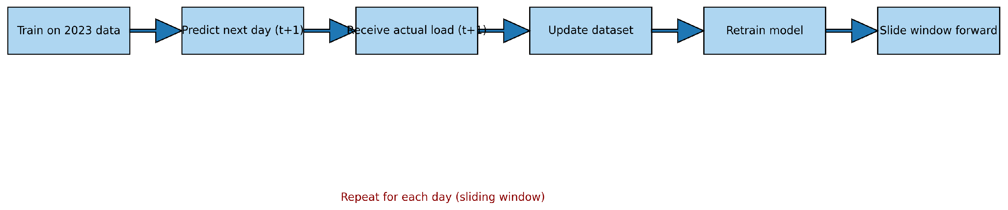
After training the model with data for 2023, we then predicted 1 day ahead. After each day, the data are retrained and then the next day is predicted. The weather is seen 7 days ahead, which is how far in advance Open-Meteo provides a forecast.

The day-ahead retraining procedure used for updating the forecasting model is illustrated in Figure 2.

Example: Suppose it is 2 June 2024. We will have total load data available up to 1 June 2024 and weather forecasts available for 7 days ahead, up to 9 June 2024. When predicting the data, we assume that the previous day’s total load is available and that the weather forecast window shifts forward. Therefore, on 3 June 2024, the available total load data will extend up to 2 June 2024, while the weather forecast will extend up to 10 June 2024. This approach is referred to as a sliding window.

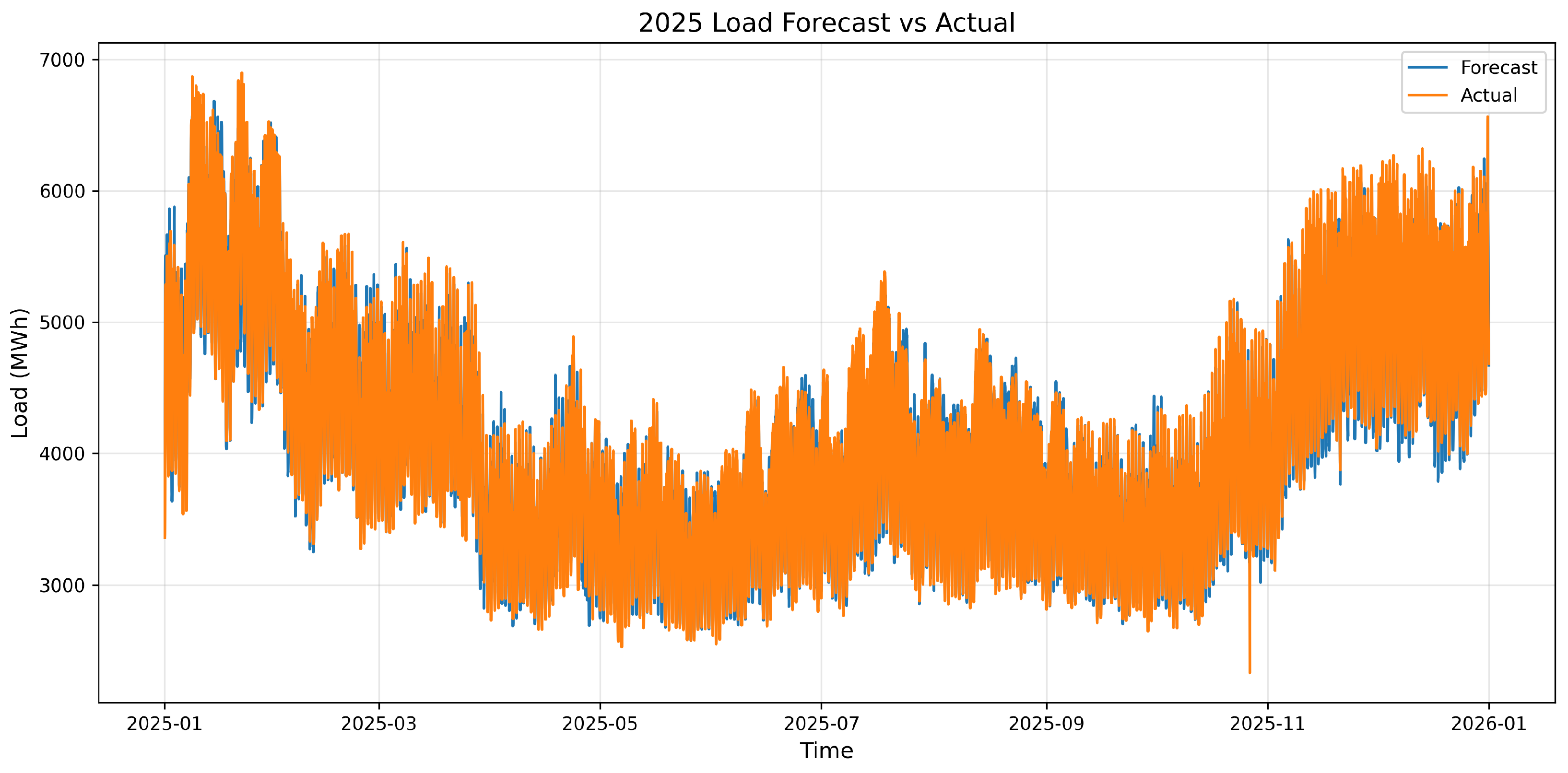
Below is the visual result of the actual load on the historical data in Figure 3.

The comparison between the predicted and actual total load values is presented table format.

The monthly forecasting performance of the proposed model is evaluated using MAE, MSE, and MAPE metrics, as presented in

Table 6. Monthly forecasting error metrics.

Month	MAE	MSE	MAPE (%)
1	142.97	33,929.59	2.71
2	113.43	21,373.51	2.49
3	121.79	25,248.18	2.93
4	117.22	27,262.14	3.25
5	98.55	18,599.30	2.85
6	93.61	15,002.39	2.51
7	96.86	14,660.99	2.34
8	67.90	7993.00	1.78
9	62.06	7210.88	1.75
10	82.48	12,740.76	2.15
11	166.99	44,820.89	3.31
12	139.32	31,679.18	2.64

. The monthly forecasting performance of the proposed model is evaluated using MAE, MSE, and MAPE metrics, as presented in Table 6.

The analysis of monthly forecasting errors reveals a clear and systematic seasonal pattern in model performance, indicating that electricity demand exhibits strong time-dependent heterogeneity.

The lowest errors are observed in late summer, particularly in August and September, where all metrics (MAE, MSE, and MAPE) reach their minimum values. This suggests that consumption during these months is relatively stable and easier to forecast, which is likely due to the reduced variability in heating and cooling demand as well as more consistent behavioral patterns.

In contrast, the highest forecasting errors occur during the winter months, especially in November, January, and December. This indicates that the model struggles during periods of higher demand volatility, which is typically driven by temperature sensitivity, increased heating requirements, and more irregular consumption patterns associated with seasonal and holiday effects.

Spring and early summer months show intermediate performance with relatively stable and moderate error levels. This reflects smoother transitions in consumption behavior compared to more extreme seasonal regimes.

Overall, the results confirm that forecasting accuracy is strongly dependent on the time of year. This supports the inclusion of calendar-based features, as they allow the model to explicitly capture seasonal structure rather than forcing it to infer these patterns indirectly from the data.

Software and Hardware

The hardware configuration is given with the following parameters:

Intel(R) Core(TM) i7-8650U CPU @ 1.90 GHz (2.11 GHz), 16.0 GB RAM,

12th Gen Intel(R) Core(TM) i5-12500H (2.50 GHz), 16.0 GB (15.7 GB usable).

4. Conclusions

This paper successfully developed a supervised machine learning framework for forecasting the hourly total electricity load of Bulgaria, utilizing gradient boosting architectures and localized meteorological features. By training the model on 2023 data and performing cross-validation against 2024 data, we achieved an average MAPE of 2.56%. Detailed monthly analysis revealed that model performance peaked during the late summer period (August and September), where error rates reached their lowest points at 1.78% and 1.75%, respectively.

4.1. Strengths of the Analysis

The primary strength of this paper lies in its computational efficiency and localized precision. By utilizing the LightGBM algorithm, the model captured complex nonlinear relationships between demand and weather variables without the prohibitive training costs often associated with deep learning architectures. Furthermore, the integration of a multi-city meteorological mean—derived from Sofia, Plovdiv, Varna, and Ruse—provided a robust proxy for national climatic trends. This approach effectively smoothed localized sensor noise while maintaining high sensitivity to the thermal inertia of the Bulgarian building stock. The results demonstrate that ensemble tree-based models remain highly competitive for national-level forecasting when exogenous variables are carefully engineered and localized.

4.2. Limitations and Future Research

Despite the high accuracy achieved, several limitations remain that provide a roadmap for future scholarly inquiry:

• Geographical Weighting: Currently, meteorological features are treated with equal weighting across the four representative cities. However, as the Bulgarian population and economic activity are heavily concentrated in specific urban hubs, future iterations should implement population-weighted weather indices to more accurately reflect the impact of temperature on aggregate demand.
• Industrial Spatial Analysis: The current model does not explicitly account for the locations of heavy industrial consumers. Incorporating spatial data regarding large-scale manufacturing sites and their specific operational schedules could further reduce error during periods of industrial shifting.
• Data Volume: While the 2023–2024 period provided a stable baseline, training on a broader historical horizon (e.g., 5–10 years) would allow the model to better learn the impacts of extreme weather events and long-term economic cycles.
• Advanced Architectures: While gradient boosting proved effective, there is significant potential in exploring attention-based models. Future work will investigate the Temporal Fusion Transformer (TFT) and other transformer architectures to determine if multi-horizon forecasting can be improved through better temporal dependency mapping and uncertainty quantification.