Proceeding Paper

Research on the Time Mutability Method for Stochastic Objects Drift Velocity Measurement—A Review †
by
Boryana Pachedjieva
1,2,*,
Petya Pavlova
2,
Dobrinka Petrova
1,2 and
Ivailo Atanasov
1,2
1
Faculty of Electronics and Automation, Technical University of Sofia, Plovdiv Brunch, 4000 Plovdiv, Bulgaria
2
Center of Competence “Smart Mechatronic, Eco-and Energy-Saving Systems and Technologies”, Technical University of Sofia, 4000 Plovdiv, Bulgaria
*
Author to whom correspondence should be addressed.
Presented at the 15th International Scientific Conference TechSys 2026—Engineering, Technologies and Systems, Plovdiv, Bulgaria, 14–16 May 2026.
Eng. Proc. 2026, 150(1), 45; https://doi.org/10.3390/engproc2026150045
Published: 21 July 2026

Abstract

The paper presents a review of research on the time mutability method for stochastic objects drift velocity measurement. The method models one-dimensional signals describing the movement of cloud structures with different types of statistical heterogeneity, without considering their evolution in the measurement interval. The main study shows the dependence of the accuracy of the measured speed V results on the number of recorded images, the type of statistical heterogeneity of the fields examined, and the measurement conditions. The obtained results are graphically illustrated.

1. Introduction

The processing of sequentially registered spatial images is increasingly becoming a successful approach for analyzing spatiotemporal data in all areas of natural sciences [1,2,3]. This is the key moment in the study of complex phenomena that are difficult to study with point measurement methods. The rapid development of methods for spatio-temporal image analysis is mainly due to the development of modern computer vision and video analysis systems, and autonomous systems, with application in medical diagnostics, remote sensing and intelligent infrastructures.
One of the complex tasks solved with Spatiotemporal Image Analysis is measuring the speed of movement of objects with a stochastic spatio-temporal structure. A typical example of such objects is cloud fields.
A special place among the methods for such type of measuring is occupied by correlation methods [3,4]. Specific to them is the rejection of the velocity field as a means of investigation and its replacement with a search for averaged (for a certain spatial region and time interval) characteristics such as drift velocity—the horizontal velocity at which a cloud field moves, or average translational velocity, average size, orientation and life of moving objects with a stochastic time-space structure, which in this case are called inhomogeneities. The drift velocity is often calculated by tracking its movement in successive images. It usually differs from ambient wind speed due to internal turbulent processes and cloud evolution.
The correlation method for processing of spatial images that are lidar or radiometric and registered in consecutive time moments by laser locators allows one to measure wind speed in the atmosphere [4,5,6]. The main methodological shortcoming of this method is the spatial heterogeneity and temporal non-stationarity of aerosol heterogeneities. As a result, correlation functions cease to be a measure of the presence of a linear statistical relationship between moving inhomogeneities observed in different spatial regions or time moments. Many attempts have been made to modify correlation methods and adapt them to spatial heterogeneity and temporal non-stationarity of the studied objects [4].
In [7], a method for a new non-correlational statistical processing of lidar or radiometric data is proposed and developed. Its purpose is to determine only the speed of movement of aerosol fields V . At the expense of this conscious limitation, the main disadvantage of correlation methods is overcome—sensitivity to the statistical heterogeneity and non-stationarity of the processed signals. This method is called the time mutability method (TMM). It is based on a new organization of the use of experimental data, namely, interpretation of the time-space realizations S r , t as time realizations in a spatial coordinate system moving relative to the Earth’s surface. This provides a more complete extraction of the information about the V from lidar or radiometric data. It is also based on the rejection of constructing spatial cross-correlation functions. In return, the construction of time mutabilities simplifies and shortens the computational procedures and leads to the main advantage of the method—insensitivity to the statistical non-stationarity and heterogeneity of the signals from the studied field.
The aim of this work is to present a summary of studies on the accuracy of TMM for measuring the drift velocity at the lower boundary of cloud fields based on model signals, without considering the time evolution.

2. Materials and Methods

To represent the accuracy of the method, the TMM is applied for processing of data obtained during thermal IR radiometric measurements of the lower boundary of cloud field horizontal velocity. The dependency of the accuracy of the results for V on the number of registered images, on the type of statistical inhomogeneity of the investigated fields, and on the measurement conditions has been investigated.
Numerical experiments based on model signals corresponding to radiometric data on horizontal thermal structures of moving cloud fields were carried out [8]. These are one-dimensional signals describing the drifting motion of cloud structures with different types of statistical inhomogeneity without considering their evolution in the time interval of the measurement. A series of one-dimensional discrete spatial realizations of the signals along the direction of motion of the fields was formed. The realizations correspond to consecutive moments in time and given drift model velocities. The different series correspond to cloud fields characterized by different, visually assessed types of statistical inhomogeneities such as mean value jump—signal type I and altering dispersion—signal type II (Figure 1). The time-discrete radiometric signals S(t) registered with a single-channel (8–12   μ m ) infrared radiometer IR-1, observing the lower boundary of different types of cloud fields at the zenith, were used. The observed area of the cloud is a circle with diameter D = H 0 / 10 , where H 0 is the height of the lower boundary of the cloud.
S ( t ) S ( t k ) ,   t k = t 0 + k 1 t 0 ,   k = 1 , K ¯ ,   K 30,000   , K 1 t 0 2   h  
Figure 1 shows one representative of each of the rows (1) with type I and type II non-stationarity.
The interval t 0 = 0.3 0.5 s in (1) is at least three times larger than the time constant of the radiometer, t 0 is the initial moment of observation. Obviously (1) contains information about the spatial and time characteristics of the observed cloud fields, as well as about their velocity.
In order to apply the time mutability method, a series of spatial realizations were constructed, “realized” at different time moments and moving with a constant model velocity V m o d = 10   m / s [8].
S m o d x , t S l , k = 1 n i = 1 n S l 0 + l 1 n + k 1 V m o d + i + 1 k = 1 , N ¯ ,   N = 2 ,   3 ,   ,   30 ,       l = 1 ,   256   ¯
In (2), l and k are indices corresponding to the spatial x and time t coordinate, and l 0 is the starting point in the initial sequence, while n is the number of measurements in (1) that are averaged to obtain a single value from (2). It is accepted t k t k 1 = t = 1 s и x i x i 1 = x = 1 m . The value of n is chosen in a way to assure that within the limits of a single visual inhomogeneity in the series (1) there fall from 5 to 10 spatial discrete values of (2). The thus-modeled sequence contains N 30 spatial realizations, registered in different moments of time, with each spatial realization containing 256 spatial discretes. A shortcoming of the modeled experimental data (2) is the fact that they are “freezing” in motion, that is, there is just a translation without time mutabilities.
We preferred this modeling approach to the method of generating sequences of random numbers with a priori specified statistical properties [9], because through the latter we would model our own ideas about the statistical properties of cloud fields. Thus, five series of type (2) were generated, characterized by different types of statistical inhomogeneity.
The general defined formula for time mutabilities [7] for sequences (2) is reduced to
I U = S x l , t k 1 S x l + ξ , t k + 1 2 ,   x l + ξ = x l + ξ U 0 ,     U 0 = Δ x Δ t ,       U = ξ U 0
The symbol 〈 〉 denotes averaging over all spatial pairs of points between which one passes with speed U and over all possible consecutive pairs of spatial realizations. From Formula (3), it is evident that the form of I U significantly differs from that of the correlation functions. The latter reach maximum values for lags corresponding to the time or spatial shifts of the two signals on which the correlation function is calculated. In contrast, I U has maximum values when S x l , t k 1 and S x l , t k 1 , and it is minimized when U approaches V m o d .
An important part of the analysis of TMM is the study of the influence of the measurement conditions on its accuracy. For this purpose, the model signals (2) are subjected to one of the following operations [10]:
(A).
quantization by amplitude at 512, 256, …, 4 levels;
(B).
decimation by spatial coordinate over 2, 4, …, 32 samples;
(C).
averaging by spatial coordinate over 2, 4, …, 32 samples.
Operation (A) corresponds to registration performed by an analog-to-digital converter for a signal that occupies a limited number of discrete levels.
Operation (B) is essentially a discretization of the signal along the spatial coordinate. The following reasons stimulated discussion of the impact of operation (B). The first one is that when the initial data is a set of two-dimensional images measured at equidistant time moments, these could be cloud images obtained by a photo camera, by microwave radar, or by a thermistor, and before TMM handling we have to discretize our data. The main question is how to choose the discretization interval x ? The second reason is that in the presence of time- and space-discrete images, it is reasonable to space-decimate data and thus to reduce the number required by TMM elementary calculation operations.
The alternative to K-fold space decimation of the signal is to replace every K successive space data point with the average value. Both operations perform low-frequency filtration on the one hand, and on the other hand lead to a reduction in the number of calculation operations.
The next step in the handling of modeled data sets (2), after performing operations (A), (B) and (C), is velocity estimation by TMM. Using (3) and the formulae given in [7] for each model data set, the cloud field velocity V c a l c N and the error ε N are calculated.

3. Results

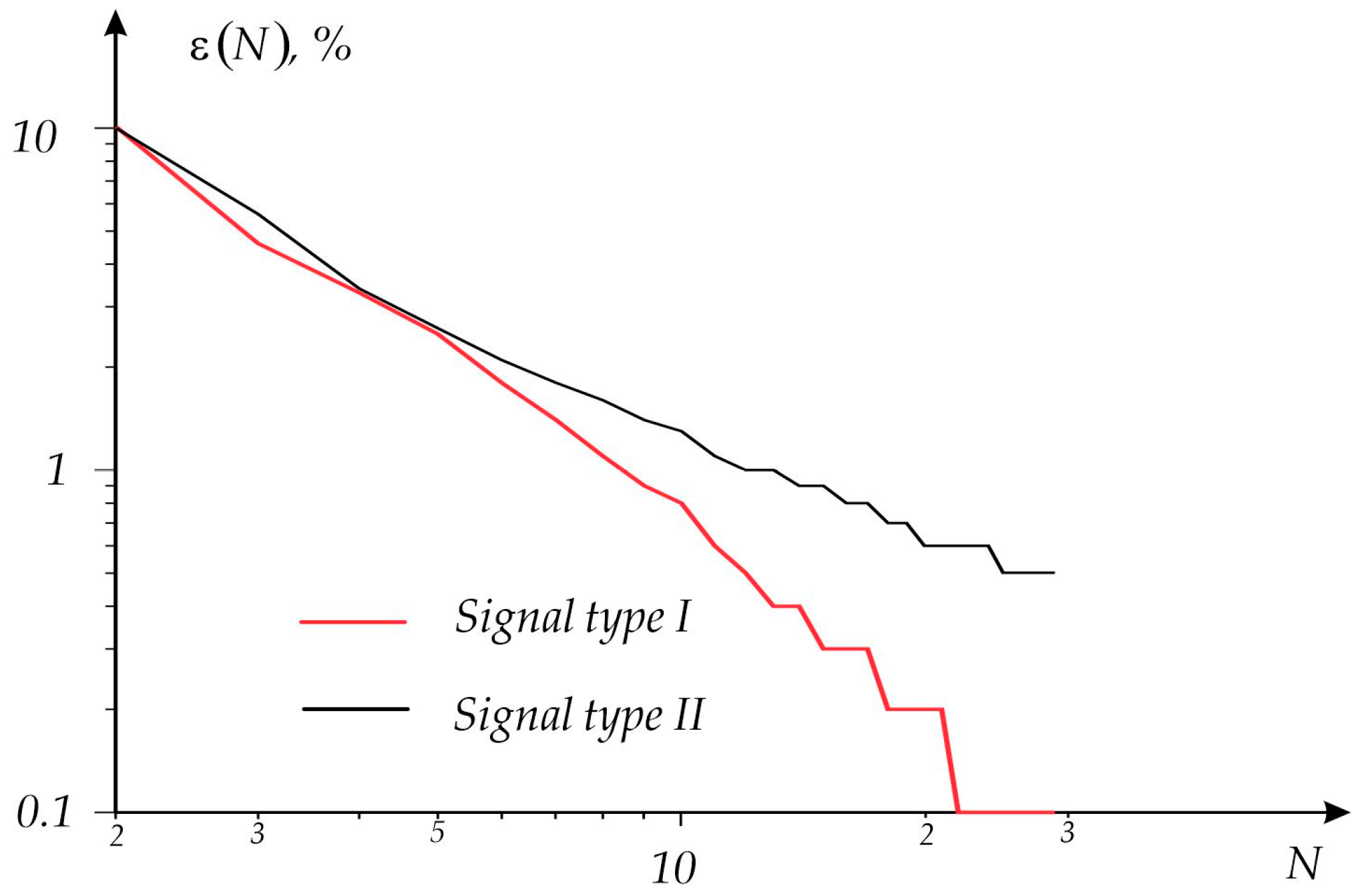
The analysis of numerical experiments shows that the calculated velocity strongly depends on the volume N of the sample (2). As an assessment of the accuracy of the calculation, the following value is accepted:
ε N = V c a l c ( N ) V m o d / V m o d · 100   ,       [ % ]
Figure 2 shows the results obtained for the models based on the signals shown in Figure 1.
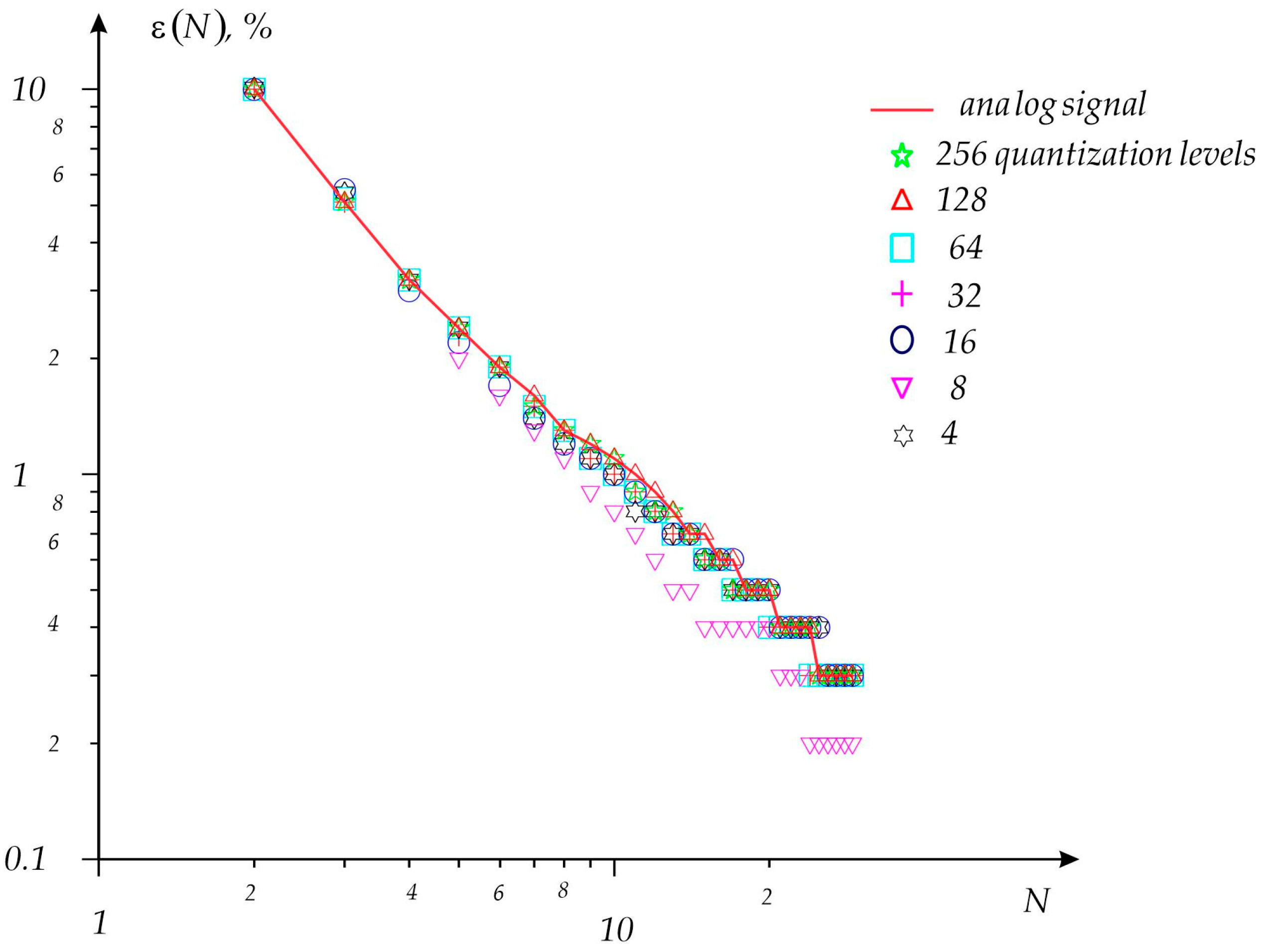
Figure 3 shows the dependencies ε N at different levels of quantization 4 Q 256 calculated for all model realizations of the signals type I and II. The calculations were performed for the source signal and for signals quantitized with Q quantization levels. An analog signal is called the source signal that is not quantitized.
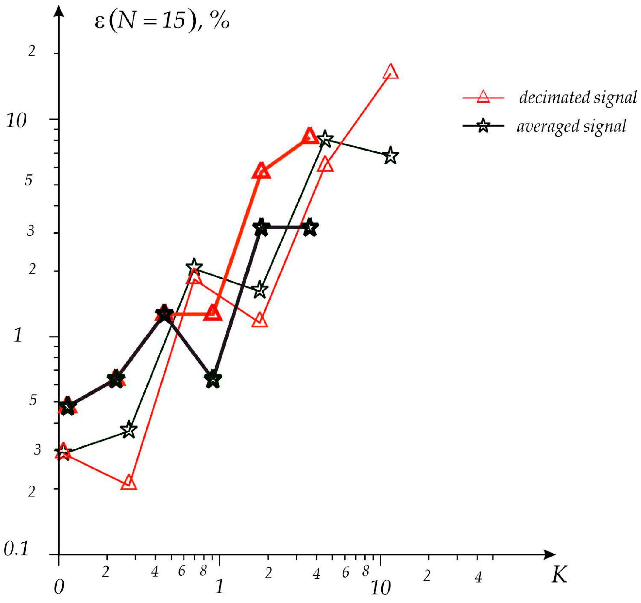
Figure 4 shows the effect of K-fold spatial decimation and averaging over K consecutive samples, applied to the same signals across N = 15 spatial realizations.

4. Discussions

The analysis of the results of processing all model signals leads to the following conclusions:
  • The type of dependency I U with respect to U strongly depends on the type of non-stationarity of the signals S x l , t k 1 and on the number of spatial signals N . An absolute minimum of I U is always observed, located in the vicinity of V m o d .
  • Regardless of the non-stationarity type of the spatial signals, the calculated velocity V c a l c N using TMM monotonously reaches for the real or model velocity V m o d .
  • To ensure 2% of the calculation error using TMM, it is enough to use more than seven spatial signals in the calculations. This requirement is not affected by the statistical properties of the signals.
  • The accuracy of the results obtained by the TMM is practically independent of the number of discrete levels occupied by the measured signal. A slight tendency toward improved accuracy is observed for lower quantization levels, within the range 16 Q 64 .
  • The type of dependence of the magnitude of the relative error on the number of spatial realizations is not affected by the number of quantization levels of the signal. This allows us to conclude that the results obtained by the TMM exhibit exceptionally high robustness with respect to the presence of noise in the recorded signal.
  • The two-fold decimation of the input signals has practically no effect on the accuracy of the results obtained by the TMM. At the same time, it leads to a significant reduction in the required computational time.
  • With four-fold decimation, the accuracy of the obtained results begins to depend on the type of non-stationarity of the input signal. A comparison of the estimates for all sets with identical statistical properties does not reveal any clearly pronounced trend. In outline, when decimation enhances the prominent elements of the signal without reducing their number, the accuracy either improves or changes insignificantly. For eight-fold decimation or higher, the TMM accuracy deteriorates significantly. If the decimated signal still contains a relatively large number of typical details, the dependence ε N remains well-defined; otherwise, it may exhibit a chaotic character.
  • The influence of space-decimation and space-averaging of the signal on the accuracy of the TVM is entirely analogous. This is illustrated convincingly in Figure 4.

Author Contributions

B.P., P.P., D.P. and I.A. were involved in the full process of producing this paper, including conceptualization, methodology, modeling, validation, visualization, and preparing the manuscript. All authors have read and agreed to the published version of the manuscript.

Funding

This research was funded by the European Regional Development Fund within the OP “Research, Innovation and Digitalization Programme for Intelligent Transformation 2021–2027”, Project No. BG16RFPR002-1.014-0005 Center of competence “Smart Mechatronic, Eco-and Energy Saving Systems and Technologies”.

Institutional Review Board Statement

Not applicable.

Informed Consent Statement

Not applicable.

Data Availability Statement

Data are available in this manuscript.

Conflicts of Interest

The authors declare no conflicts of interest.

References

  1. Jahne, B. Spatio—Temporal Image Processing. Theory and Applications; Springer: Berlin/Heidelberg, Germany, 1993. [Google Scholar]
  2. Galic, Z. Spatio-Temporal Data Streams; Springer: New York, NY, USA, 2016. [Google Scholar]
  3. Matvienko, G.; Zadde, G.; Ferdinandov, E.; Kolev, I.; Avramova, R. Correlation Methods for Laser-Location Wind Velocity; Science: Novosibirsk, Russia, 1985. (In Russian) [Google Scholar]
  4. Matvienko, G. Lidar measurements of wind speed using the stochastic structure of aerosol fields. Opt. Atmos. [Atmos. Opt.] 1988, 1, 3–15. (In Russian) [Google Scholar]
  5. Kozintsev, V.; Ivanov, S.E.; Belov, M.L.; Gorodnichev, V.A. Laser correlation method with adaptive choice of measuring base for on-the-fly measurements of wind velocity. Atmos. Ocean. Opt. 2012, 25, 263–268. [Google Scholar] [CrossRef]
  6. Liu, S.; Li, G.; Xie, H.; Wang, X. Correlation Characteristic Analysis for Wind Speed in Different Geographical Hierarchies. Energies 2017, 10, 237. [Google Scholar] [CrossRef]
  7. Ferdinandov, E.; Stoikova, E.V. Method of Laser Sounding of the Atmospheric Dynamics. Bulg. J. Phys. 1984, 11, 58–69. [Google Scholar]
  8. Pachedjieva, B.; Tsanev, V.; Ferdinandov, E. Time Mutability Method for Cloud Field Drift Velocity Measurements. Compt. Rend. Acad. Bulg. Sci. 1996, 49, 49–51. [Google Scholar]
  9. Davenport, W.B.; Root, W.L. An Introduction to the Theory of Random Signals and Noise; IEEE Press: New York, NY, USA, 1987. [Google Scholar]
  10. Pachedjieva, B.; Tsanev, V.; Ferdinandov, E. Influence of the Measurement Conditions on the Accuracy of the Time Mutability Method for Cloud Field Drift Velocity Estimations. Compt. Rend. Acad. Bulg. Sci. 1996, Tome 49, 47–50. [Google Scholar]
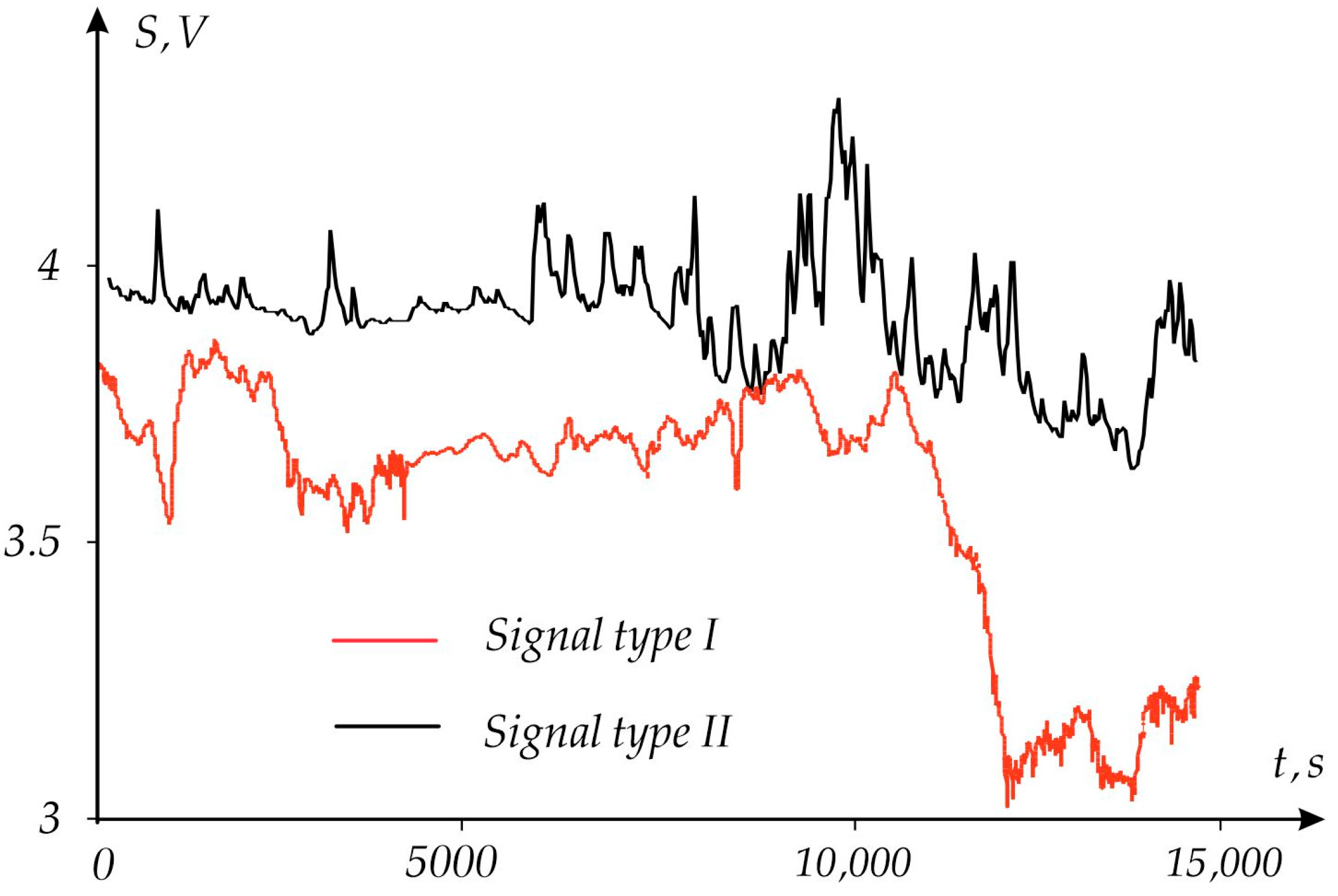
Figure 1. Graphics of two signals of different types of non-stationarity.
Engproc 150 00045 g001
Figure 2. Dependences ε N calculated using data set (2), modulated by the signals type I and type II.
Engproc 150 00045 g002
Figure 3. Dependences ε N for signals type I and type II with parameter the number of quantization levels Q. The source signal is denoted as analog signal.
Engproc 150 00045 g003
Figure 4. Dependences ε N = 15 for signals type I and type II with parameter K.
Engproc 150 00045 g004
Disclaimer/Publisher’s Note: The statements, opinions and data contained in all publications are solely those of the individual author(s) and contributor(s) and not of MDPI and/or the editor(s). MDPI and/or the editor(s) disclaim responsibility for any injury to people or property resulting from any ideas, methods, instructions or products referred to in the content.