Content Reuse Analytics and AI Readiness Assessment for Content in the Maritime Product Component Supplier Domain ^†

Abstract

This paper addresses content reuse analytics and AI readiness assessment in the domain of maritime product component suppliers, with a particular emphasis on RAG processes and the role of reuse-related metrics. Built on previous research in technical communication, content engineering, and information architectures, the paper investigates how the structure, similarity characteristics, and metadata of maritime component documentation interact with RAG mechanisms when contextual information is supplied to LLMs in AI-based delivery scenarios. The paper investigates how various parameters, such as content similarity, influence retrieval accuracy and output quality while analyzing patterns of topic reuse.

1. Introduction

Digitalization and the adoption of Artificial Intelligence (AI) are gaining increasing significance across industries, including the domain of technical communication. Technical communication typically relies on a topic-based organization of content within Component Content Management Systems (CCMSs), most commonly using XML-based formats [1]. At present, AI in technical communication is employed for tasks like content generation or machine translation [2]. Beyond this, its scope of application can be extended to include the analysis of data and content, particularly with regard to assessing their suitability for AI-driven delivery processes. This topic has been explored in related research work, which provides the foundation for the work presented in this paper [3].

In the broader context of digitalization and AI, Retrieval-Augmented Generation (RAG) is emerging as an increasingly relevant approach within technical communication [4]. RAG combines large language models (LLMs) with targeted retrieval of authoritative sources to produce context-grounded, verifiable outputs [3]. As technical communication increasingly relies on AI-assisted content delivery, RAG has become essential for ensuring accuracy, consistency, and traceability in complex and rapidly evolving domains.

The content and data used for this project originate from a supplier of components for maritime products like couplings. It is a German mid-size engineering company based in Herne with a global presence. They specialize, among other things, in manufacturing for marine technology, which is the focus of the content that was used for this project. The content is written in German, translated into customer-specific languages, but labeled with metadata in both German and English [5].

2. Project Goals

The overall objective of this paper is to analyze current patterns of content reuse and their suitability for AI-based applications.

To this end, when evaluating the suitability of content for RAG processes, AI-supported analyses of content reuse represent a potential area of interest in technical communication. Such analyses could investigate where and how often the topics are used or whether something like standard topics or redundant metadata can be identified. Corresponding research and analytical approaches have been introduced earlier as report exchange (REx) analytics [6,7] and serve as a basis for the AI-enhanced reuse analytics in the present publication.

The results of these analyses could, in turn, support conclusions regarding the suitability of the content for AI-driven use cases or other types of digital information services.

Beyond that, another line of investigation examines how topic and ensemble sizes and sub-ensemble filtering affect retrieval sharpness and response quality in RAG delivery. Here, ensemble size refers to the number of topics vectorized in one database collection.

3. Method and Process

The methodological approach follows the overall workflow of the so-called PIAI!-Lab framework, defined by one of the authors for academic content analytics [3]. Accordingly, the analysis is conducted within a Python-based environment (version 3.10.11) and follows the principles of Vibe Coding, which supports iterative, code-driven analytical procedures [8]. In addition, the approach is inspired by the established phases of the Data Science Lifecycle and is further shaped by the specific analytical requirements of the project (Figure 1) [9].

3.1. Phase 1: Data Examination and Data Acquisition

The first phase (Figure 1) focuses on the systematic examination and acquisition of the available data. The dataset primarily consists of assembly manuals, which form the basis for the subsequent analytical steps. A central aspect of this phase is the analysis of the available XML structure, as it determines how both content and metadata can be accessed and processed. This examination also reveals how individual topics are embedded within or reused across multiple master documents, providing insights into the overall content organization.

In this case, the document refers to manuals created for customer-specific orders. The data were organized in a consistent manner. Each document contains a main directory with a subfolder holding all related topics. For every topic, two XML files are available: a content file and a metadata file. The metadata follows a standardized structure, with the first <attributeblock> containing system-generated information, such as the author, and subsequent <attributeblock> containing content-related metadata, for example, “Installation Instructions”, as extrinsic information metadata. The content-specific metadata is particularly relevant to the project objectives, as it enables the categorization and filtering of topics for subsequent analysis.

Additionally, each document includes a document structure folder representing the master document exported from the CCMS. The folder contains a metadata XML file with the same structure as the topic metadata and a document structure file describing the document structure. The same structure is given for 102 documents, comprising around 865 topics.

3.2. Phase 2: Data Cleaning and Data Preparation

The second phase focuses on improving data consistency and preparing the content for automated processing. Therefore, the content is normalized without XML markup. This normalization process ensures that the data can be processed and analyzed reliably in the subsequent vectorization phases.

Additionally, a structured metadata overview in Excel was created. It was categorized according to the PI classification [10] in order to provide a comprehensive overview and to prepare metadata for integration into a database environment. An initial analysis of the content revealed that assigned metadata were, in some cases, not as specific as recommended by the PI-classification methodology.

Based on these findings, a common baseline database structure was developed in coordination with other project groups. This structure was subsequently adapted by each group to fulfill the specific analytical requirements of the respective use case.

3.3. Phase 3: Data Integration and Data Transformation

The third phase focuses on the systematic integration and transformation of the previously processed data into two complementary database systems: a relational database (MariaDB) [11] and a vector database (Qdrant) [12]. By organizing the data in this manner, it becomes possible to examine data relating to the research objective.

To support this process, two CSV files are generated as outputs. A Python-based program parses each document structure to identify referenced topics and extracts detailed metadata from the associated metadata.xml files. In addition, topic-specific metadata and word counts derived from the normalized content are collected. The resulting CSV data is then imported into a MariaDB instance using automated Python scripts. During this process, data are inserted or updated across four relational tables. Potential duplicate entries are detected and merged automatically to ensure data consistency.

Finally, the normalized content and the structured data stored in the relational database are used to populate the Qdrant vector database. MariaDB supports the vectorization process by providing product–topic relationships, which enable the creation of product- and document-based collections within Qdrant.

3.4. Phase 4: Exploratory Data Analysis

The final phase is dedicated to exploratory data analysis and the systematic examination of both the company’s CCMS data and the AI readiness of the content. The results of these analyses are discussed in the Chapter Key Findings—CCMS KPI Analysis.

The analysis of CCMS-related KPIs is guided by customer-specific research questions defined in coordination with the company. These requirements are addressed sequentially, with each question examined individually. The analytical foundation for this step consists of the database and the normalized content generated in the previous phases. The outcome derived from this analysis also serves as a basis for assessing the AI readiness of the data.

The evaluation of AI readiness is conducted using vectorized content stored in the vector database. Similarity-based calculations of ensemble properties, including Similarity Width (SimWidth) and Similarity Difference (SimDiff) defined in [3]. They were assessed across multiple threshold settings to examine the structure and separability of the content. In addition, the effect of varying ensemble sizes is analyzed for selected examples using a simulated RAG process, and the response quality of different LLMs is viewed. This combination of analyses provides a comprehensive perspective on the suitability of the data for AI-supported delivery applications.

3.5. Tools and LLMs

A range of software tools was used to support data processing, analysis, and documentation throughout the project. Visual Studio Code (version 1.126) served as the primary environment for scripting and code development. Database management and storage were handled using MariaDB by XAMPP and the Qdrant vector database. JupyterLab was used for documentation and script execution as the so-called PIAI!-Lab, while Microsoft Excel supported the inspection and validation of generated CSV outputs.

Several LLMs were used for different analytical purposes. For RAG, models from Anthropic with Claude Sonnet 4 and Opus 4, OpenAI with GPT-5 and GPT-4o, as well as Google with Gemini 2.5 Flash, were evaluated. In the context of Vibe Coding, a separate set of LLMs was used, comprising Anthropic’s Claude Sonnet 4.5 and Opus 4.5, alongside OpenAI’s GPT-5.2.

4. Key Findings

4.1. CCMS KPI Analysis

In the following, a selected subset of results from the project is presented. The focus is placed on findings that are particularly relevant to the evaluation of the CCMS data and its usage characteristics. The term question in this context refers to the company-specific questions introduced in Chapter Phase 4: Exploratory Data Analysis. Moreover, for each analysis, an accompanying CSV file was generated to enable further examination beyond the presented results.

4.1.1. Question 1: Topic Usage and Reuse Frequency

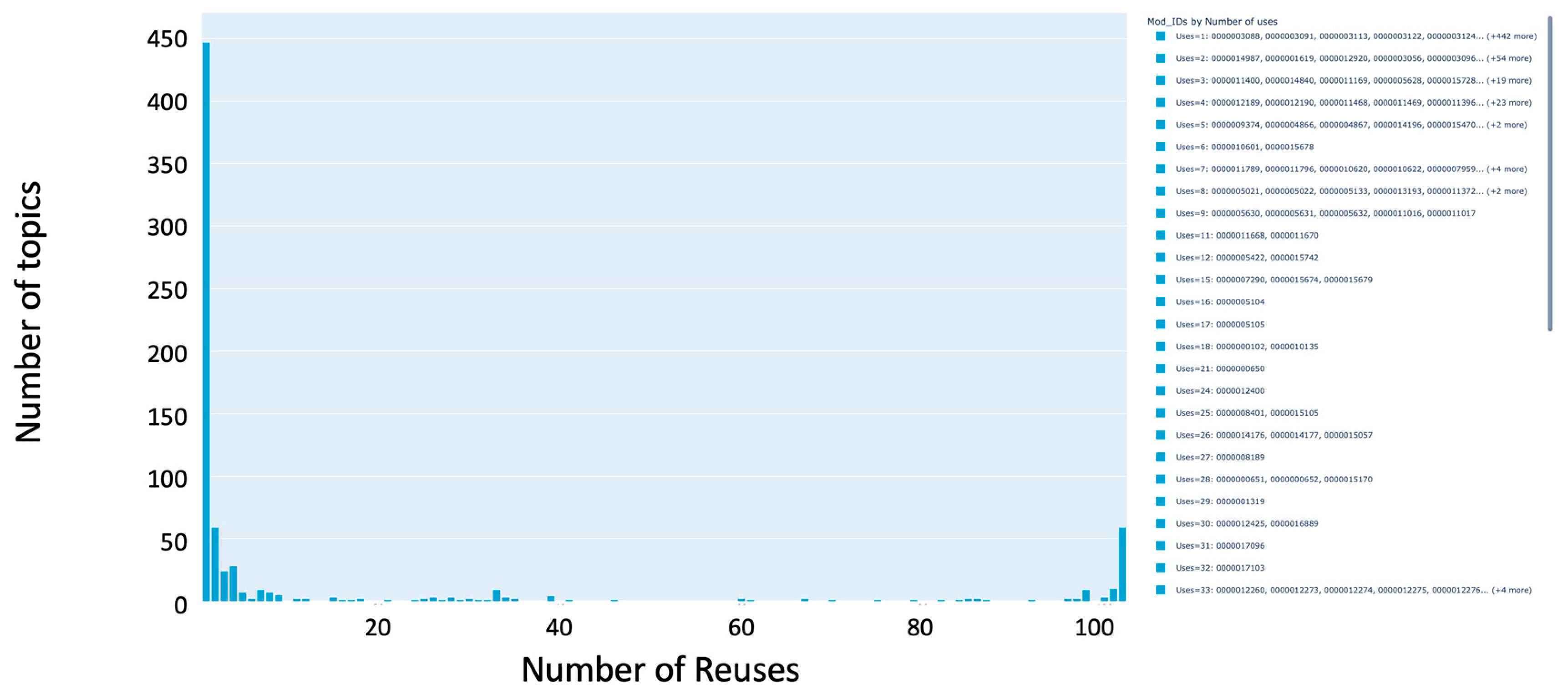
The first analysis addresses the question of which topics are used and how frequently they are reused across documents. It also serves as a characterization step for the investigated content and supports the understanding of its behavior in the following AI readiness analytics. As shown in Figure 2, the distribution of topic (re-)use number is illustrated using a bar chart, where the x-axis represents the number of times a topic is used and the y-axis indicates the number of topics corresponding to each usage frequency.

The results show a strongly left-skewed distribution. Approximately 450 topics are used only once, while around 60 topics appear twice. Beyond this point, the number of topics decreases rapidly as reuse frequency increases. At the same time, a small number of topics exhibit exceptionally high reuse rates. These topics, located at the right end of the distribution, can be considered standard topics that are repeatedly reused across multiple documents, indicating a high level of content standardization within the CCMS.

This analysis is particularly helpful as it provides insights into content reuse patterns and the degree of standardization within the CCMS. It identifies topics with a lower reuse rate, while highly reused topics indicate standard topics that are critical for consistency and maintenance.

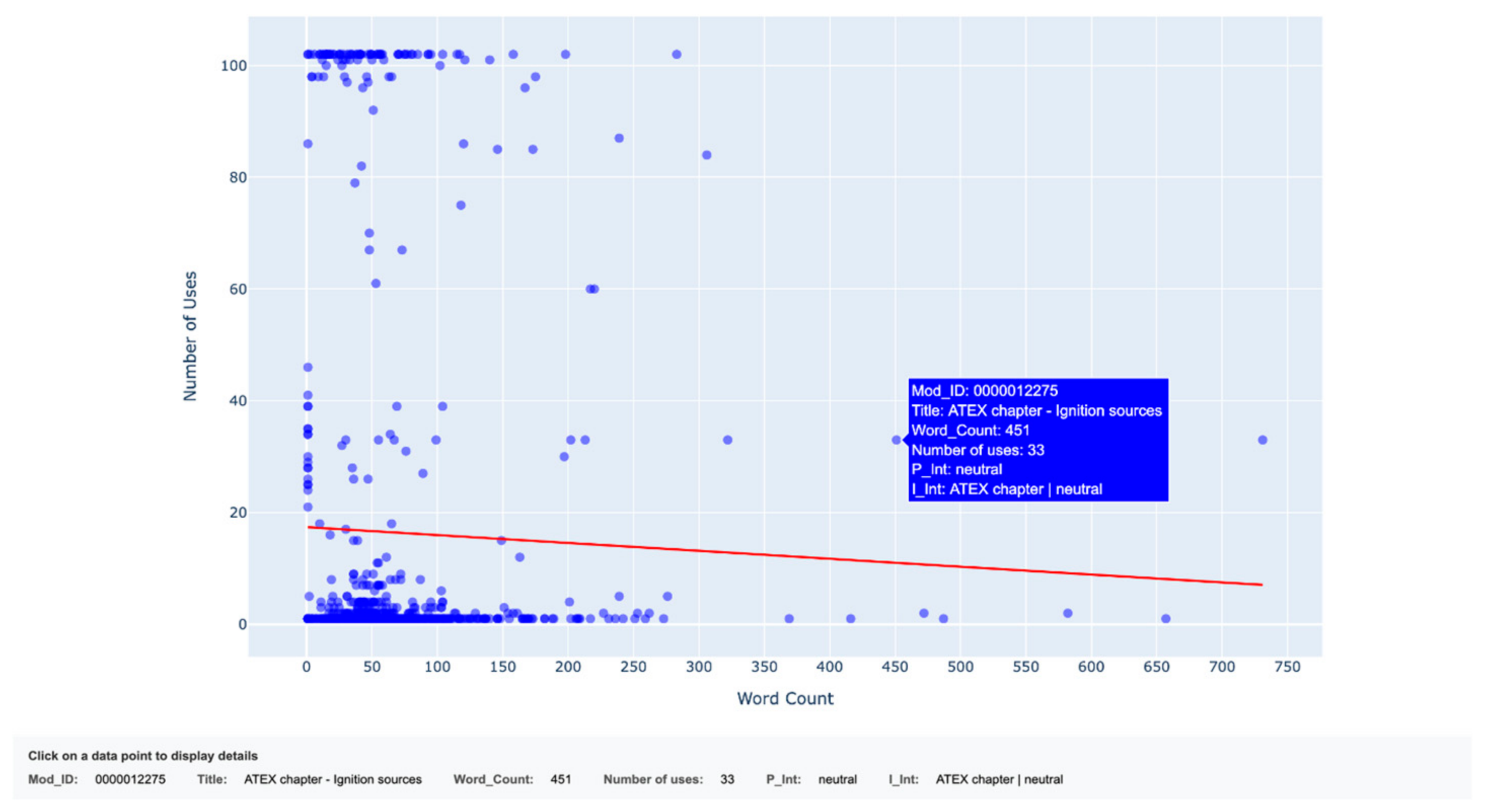
As an extension of the first analysis, a scatter plot was used to examine the correlation between topic length and reuse frequency. As shown in Figure 3, the x-axis represents the word count of each topic, while the y-axis indicates the number of times the topic is reused across documents. Each data point corresponds to an individual topic, and the overall distribution of points allows for an assessment of potential correlations between topic size and reuse behavior.

The results indicate that higher reuse rates are generally associated with topics of smaller content size. However, the large number of topics characterized by both low reuse rates and small size reflects the variant-specific content creation processes typical of manufacturing environments with a high degree of product specificity. As expected, large topics exhibit comparatively low reuse rates. Overall, the observed reuse behavior confirms the general tendency previously identified in REx analytics within the machinery industry.

The interactive design of the visualization further supports the analysis. Hovering over individual data points reveals additional metadata, such as topic ID, title, word count, and number of uses, as illustrated in the figure. Selecting a data point opens a detailed information panel at the bottom of the page, providing further insights into the corresponding topic. Most visualizations were implemented as interactive elements to align with the analytical requirements and practical needs of industrial partners.

4.1.2. Question 2: Distribution of Explosion Safety—Related Topics Across Documents

The second analysis addresses, as an example for industry-relevant content analytics, the specific question of how many topics related to explosion safety (ATEX [13]) exist and in which documents they are applied. To answer this project-specific question, two complementary analyses were conducted: a metadata-based analysis and a keyword-based analysis. The keyword-based analysis serves as a validation step to assess the completeness of the topic metadata.

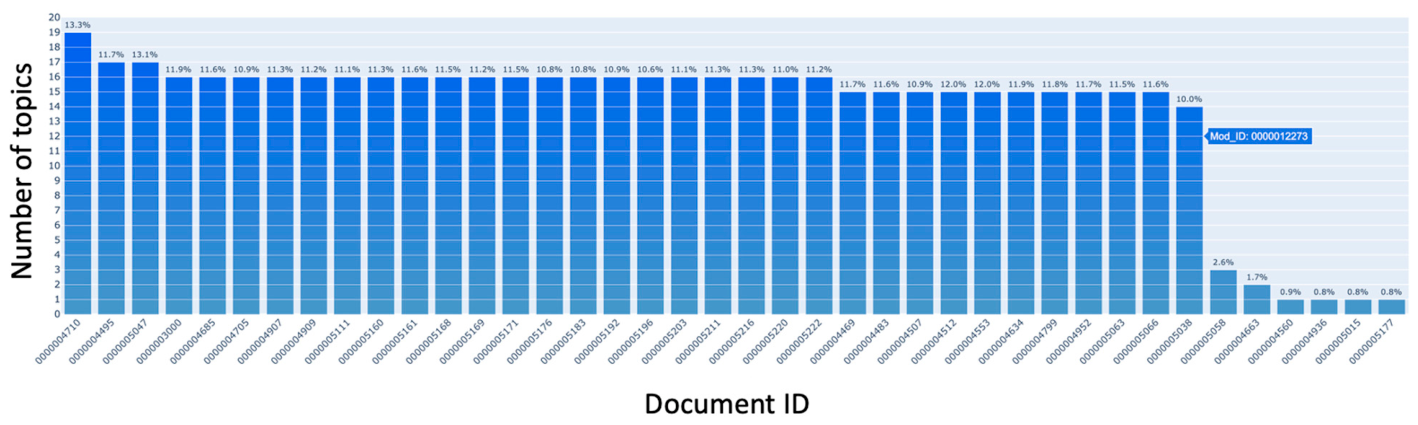
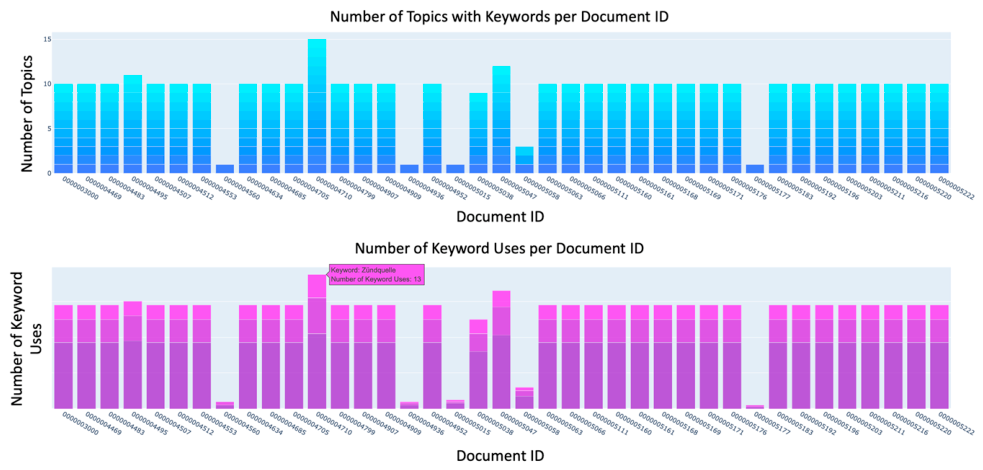
The metadata-based analysis reveals a clear clustering of documents with respect to explosion safety topics. As illustrated in Figure 4, documents on the left side of the distribution contain a relatively high number of explosion safety-related topics, whereas documents on the right side only include a limited number of relevant topics.

The keyword-based analysis of all documents, on the other hand, shows a similar distribution. The keywords like “explosion” were given by the company. As shown in Figure 5, the upper bar chart illustrates the number of topics per document in which explosion safety-related keywords occur, while the lower bar chart depicts the total number of keyword occurrences for the previously analyzed topics per document.

The strong alignment between these two analyses indicates a high level of agreement between the metadata of topics per document and actual content. This suggests that the ATEX conformity metadata reliably reflects the presence of explosion safety-related information at the module level. Consequently, the metadata can be considered as a basis for identifying and analyzing explosion safety content across documents, while the keyword-based analysis serves as an effective validation of metadata completeness and consistency.

4.1.3. Question 3: Overview of the Usage of Topics in Documents and Products

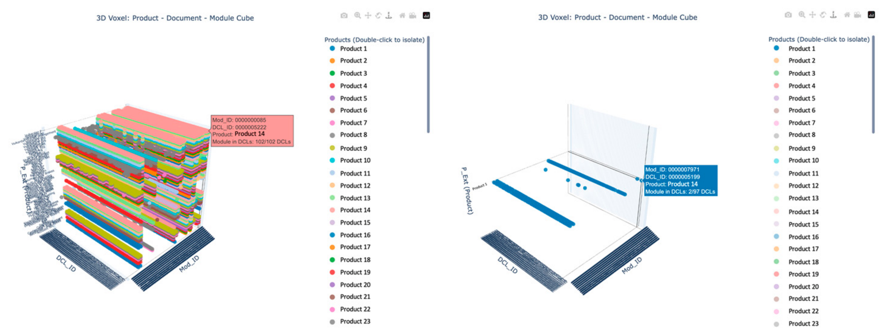
The final analysis of content management properties addresses the question of whether there are topics that are used across all documents of a given product. To enable a simultaneous exploration of topic usage patterns across documents and products, a 3D interactive visualization was used. This visualization allows for examining the relationships between topics, documents, and products.

As illustrated in Figure 6, the visualization is generated as a three-dimensional voxel structure. The x-axis represents the topic IDs, the y-axis corresponds to the document IDs, and the z-axis illustrates the extrinsic product metadata (P_Ext). Each data point, therefore, represents the occurrence of a specific topic within a particular document for a given product. The interactive design allows filtering by individual products, enabling a focused analysis of topic usage within a single product’s documentation set, as shown in Figure 6.

By hovering over individual data points, detailed information is provided, including the number of documents in which a topic is used in comparison with the total number of documents available for the selected product. Topics whose data points form a nearly continuous line across the document axis indicate usage in almost all documents associated with that product. Such linear patterns indicate product-wide topic reuse. There is a relatively high number of documents per product because the documents are produced for customer-specific orders.

This visualization and corresponding analysis support the identification of potential standard topics that are consistently applied across all documents of a product. These topics can be interpreted as standard topics.

4.2. AI Readiness

For the core project research area, an overview of Similarity Difference (SimDiff) and Similarity Width (SimWidth) introduced in [3] of the available ensembles was generated. SimDiff measures how strongly similarity values vary, for example, how homogeneous the similarity structure is. This means: If the SimDiff is low, topics are more similar. If the SimDiff is high, topics are less similar.

The SimWidth describes the number of topics in the ensemble that lie above a specific similarity threshold. This number corresponds to the context given to a RAG process in case of a request as described in [3].

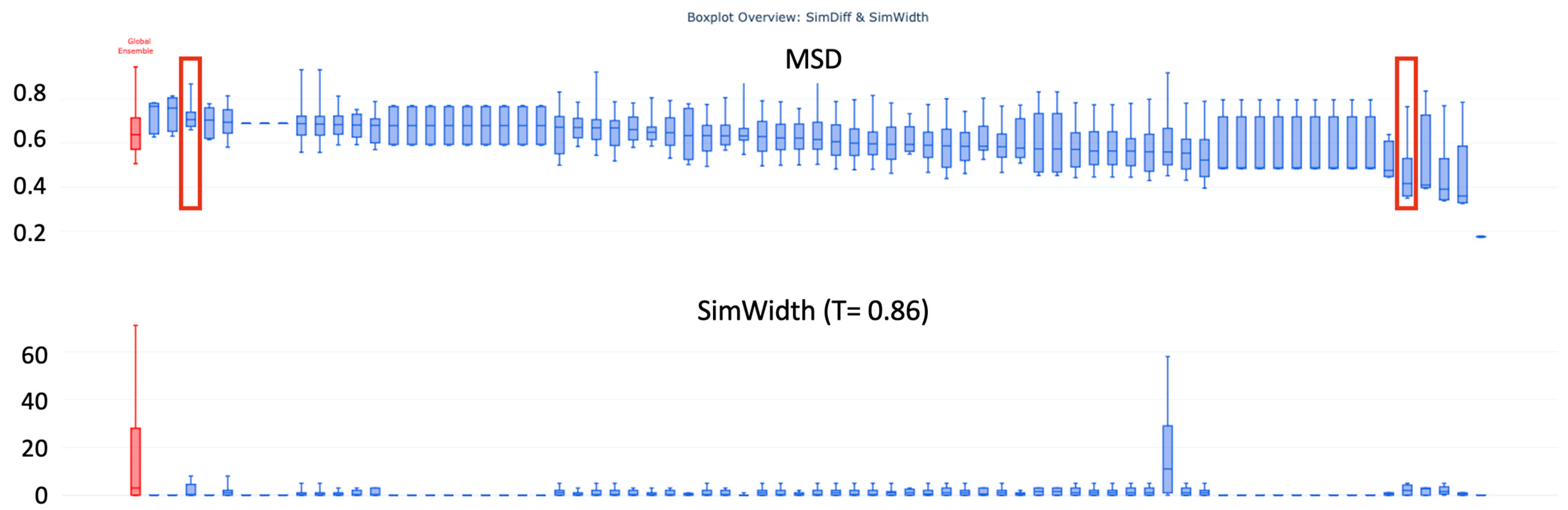
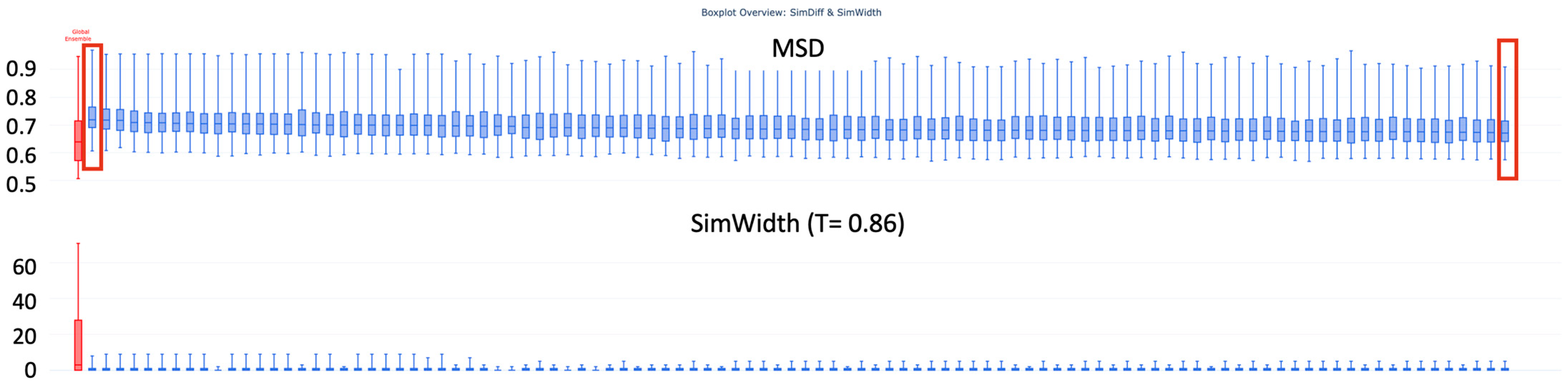
Figure 7 shows box plots of the Mean SimDiff (MSD) (on the top) and SimWidth at a threshold of 0.86 (on the bottom), comparing individual product sub-ensembles (marked blue) with the global ensemble (marked red) arranged in descending order.

The graph reveals variations between products. A number of products show higher MSD values, suggesting the presence of a larger number of distinct topics. The global ensemble shows, in consequence, a quite broad similarity distribution, as it compares all available topics. Nevertheless, the investigated product ensembles have, in many cases, a high (compressed) MSD value distribution, which is above 0.6. Deviations can be identified and investigated by content architects. As a consequence, the ensembles exhibit low similarity widths, indicating that topics are quite distinct, and therefore RAG processes will reveal answers generated from a small number of context topics. Also, in this case, the discovered single deviation and SimWidth peak can be further investigated.

In contrast, Figure 8 compares document-level sub-ensembles (marked blue) with the global ensemble (marked red). The analysis reveals that on the document level, content is much more homogeneous at high MSD values, showing more stable similarity patterns and fewer extreme variations. The global ensemble is more heterogeneous, showing larger spread and width in high similarity values. This is indicative of lower semantic distinctiveness, i.e., a certain number of linguistically similar topics.

For the first product-related data set in Figure 7, based on the SimDiff and SimWidth analysis depicting the boxplot overview, two sub-ensembles with comparably high and low Mean Similarity Difference (MSD 0.7 and 0.4) were selected.

For each selected case, a report of an RAG query pre-test was generated, which contains the user request and the retrieved context. The retrieved context corresponds to the content with the highest cosine similarity score relative to a predefined threshold. The RAG report includes the responses generated by different LLMs. Within the scope of this project, five LLMs were evaluated.

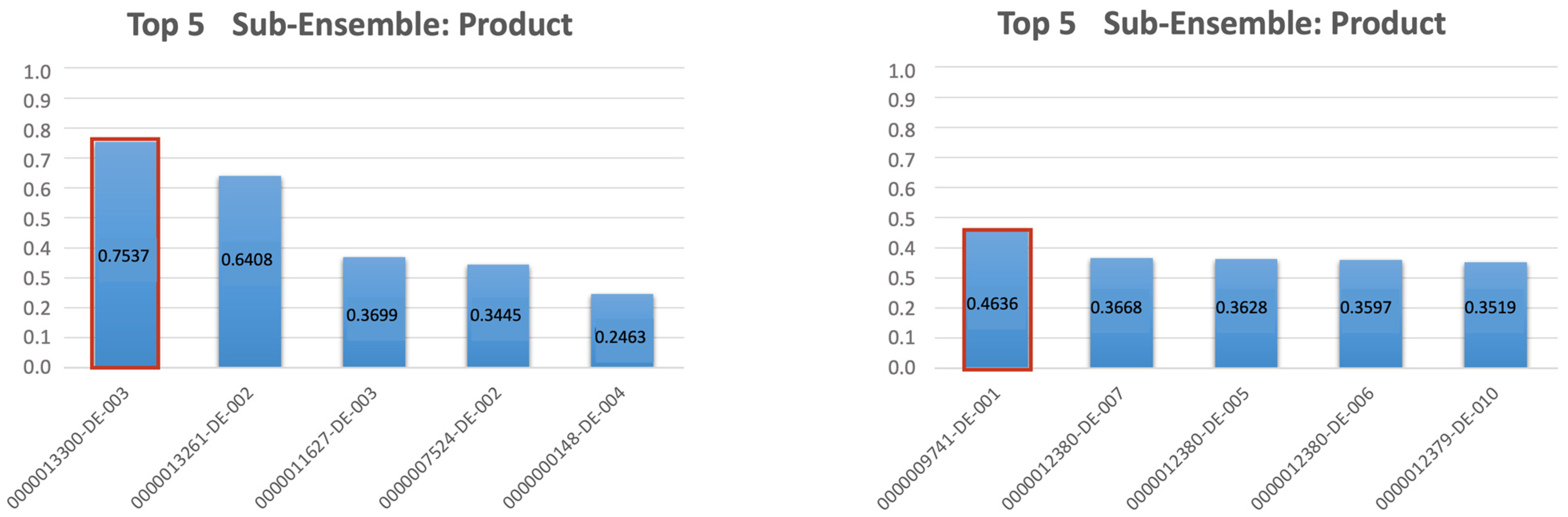
First, a product sub-ensemble with a high MSD of 0.7 was examined by a request extracted from the topics selected for the pre-test. The same request was submitted to the global ensemble. The original question was in German, being consistent with the language of the content. In this first request pre-test, both for the sub-ensemble and the global ensemble, the correct topic was retrieved as the primary response (marked with the red boxes in Figure 9). Regarding the response quality, all evaluated LLMs produced correct responses. However, in most cases, the answers included more information than required, which may potentially confuse users. Additionally, structural differences across LLMs were observed. For example, some models provided short summaries or explicitly mentioned the topic from which the information was derived. From these observations, it can be concluded that sub-ensembles with higher MSD values tend to be easier for the retrieval process to separate and result in more precise retrieval behavior, particularly when comparing sub-ensembles to global ensembles.

Secondly, a product sub-ensemble with a low MSD of 0.4 was analyzed. For the product sub-ensemble, the correct topic was retrieved as the primary result (Figure 9). Therefore, the LLM response was correct. In contrast, for the global ensemble, the correct topic was not among the top five topics with the highest cosine similarity values. Therefore, the generated answers were incorrect. In conclusion, the criteria by which sub-ensembles are generated seem to be more meaningful than MSD. The results show that with a lower MSD, the cosine Similarity Difference between these topics is much smaller. Therefore, it is much more difficult to find a threshold that specifies only one topic as context. With the global ensemble, the result is worse because many more topics could be retrieved as context.

For the analysis of the document sub-ensembles, the ensemble with the highest (MSD 0.72) and the lowest MSD (0.67) were chosen. As indicated by the MSD values, the variance was relatively small; however, it was still assessed for completeness.

For the sub-ensemble with the highest MSD, the following has been observed. For both the sub-ensemble and the global ensemble, the correct topic was chosen as context. With a threshold of 0.5, the sub-ensemble had better results than the global ensemble. In conclusion, response quality improved with fewer “wrong” topics selected as context.

For the request test of the document sub-ensemble with the lowest MSD, for both the sub-ensemble and the global ensemble, the correct topic was retrieved as context. Therefore, the response quality did not differ. In conclusion, in this specific case, if the MSD of the sub-ensemble and global ensemble are more similar, the results tend to get more similar too.

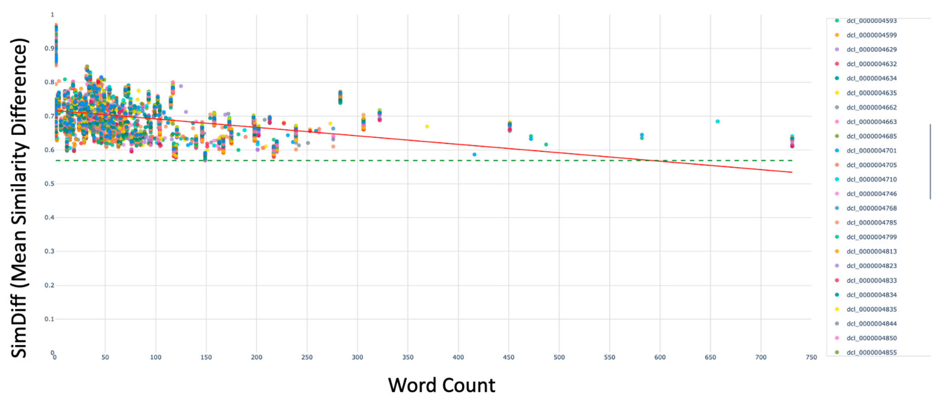
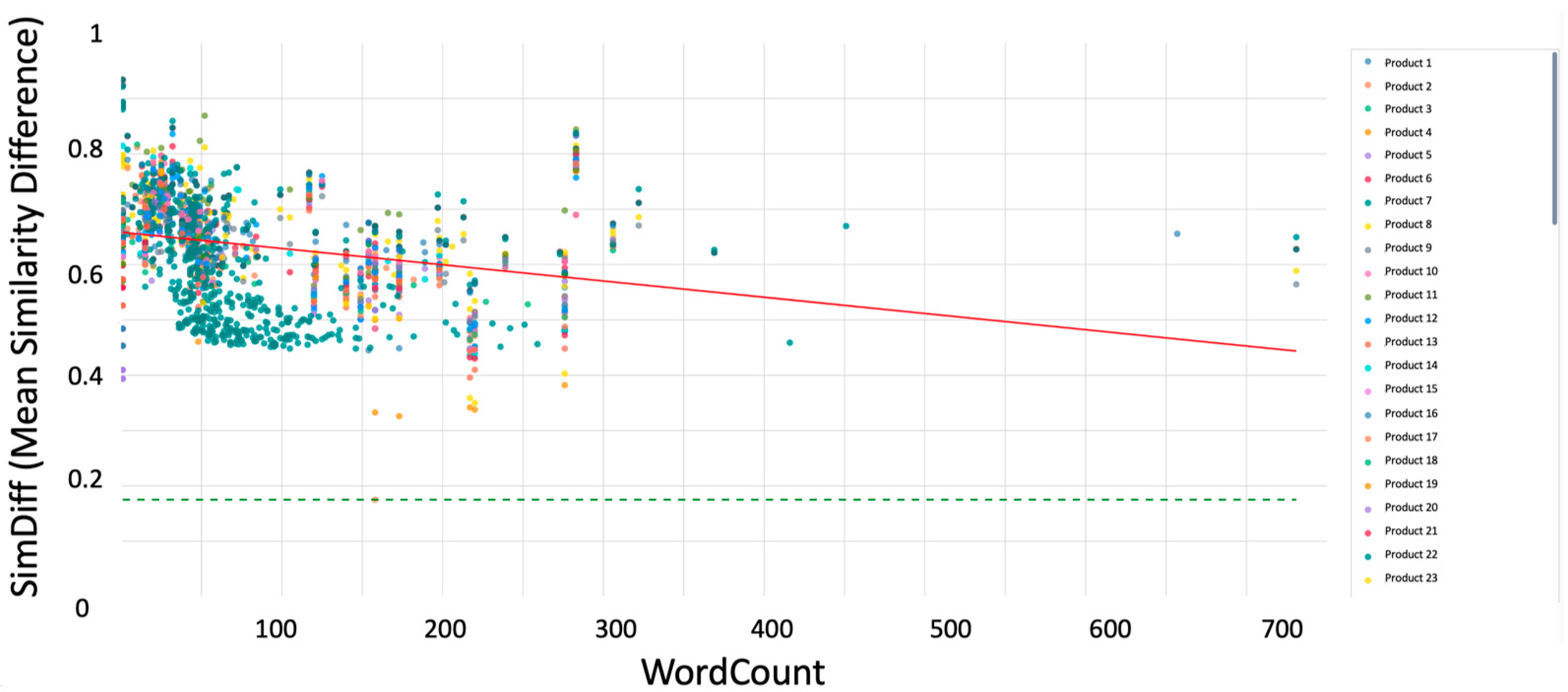
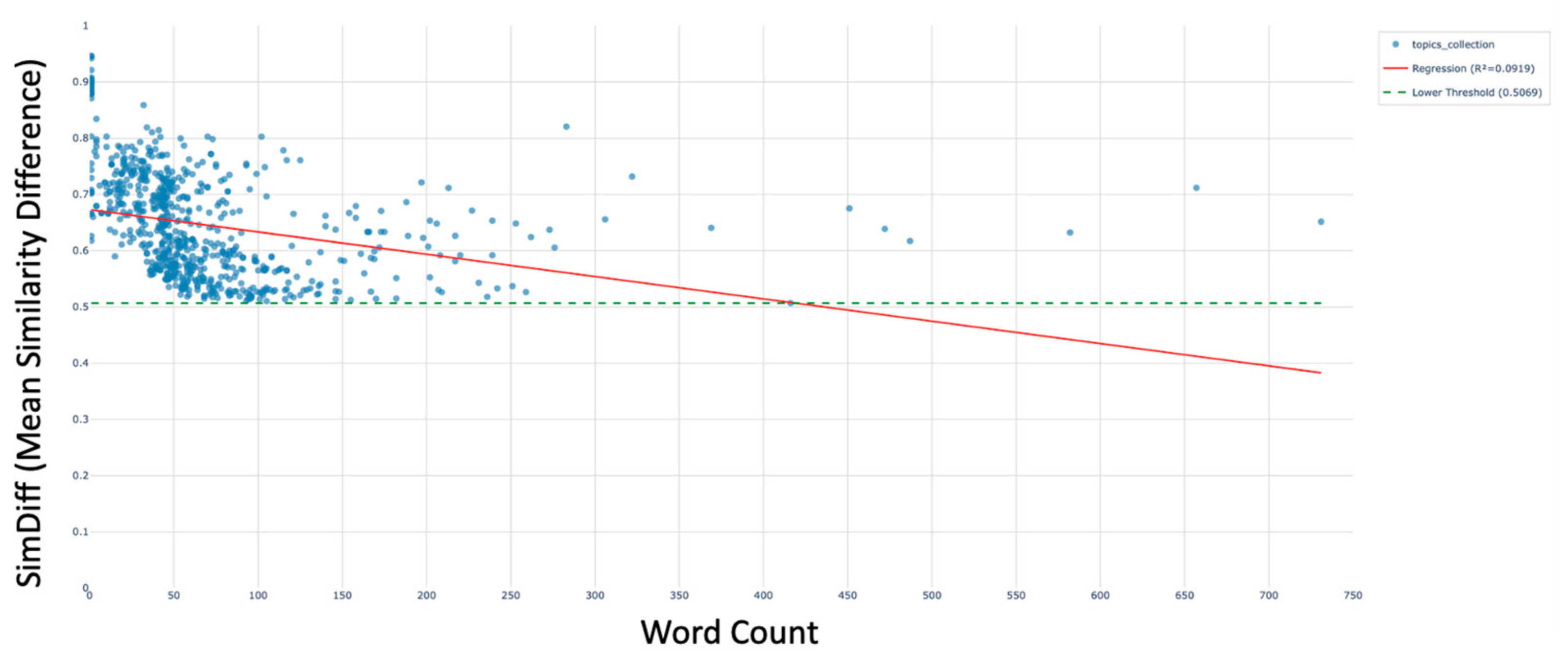
Based on these results, the question arose as to whether topic size provides any insight into AI readiness in the context of MSD. Therefore, scatter plots were generated, revealing the correlation between topic size and MSD for the global ensemble and the sub-ensembles. For the global ensemble (Figure 10), smaller topics generally clustered towards higher MSD values, while distinct outliers with low MSD were detectable. Similar tendencies appeared for the document sub-ensembles (Figure 11). For the product sub-ensembles (Figure 12), there were more outliers with higher and lower MSD values. This could be because there were generic topics but also highly specific topics in those sub-ensembles.

5. Summary and Outlook

5.1. Summary

The used methodology of ensemble properties has proven to conduct AI-supported analyses of content reuse, which deliver results for architectural content development. These analyses can support conclusions for content management and classical content delivery by showing, for example, errors in metadata allocation or for understanding and improving reuse behavior.

For AI-based delivery in RAG processes that concerns retrieval sharpness, the ensemble sizing influences retrieval sharpness, which is proven quantitatively and qualitatively by ensemble properties such as Similarity Difference (MSD). Within the scope of this project, the results indicate a tendency towards higher MSD values in product sub-ensembles that correspond to more accurate retrieval.

This means that topic-based delivery, including precise and correct metadata architectures, allows for reducing the global ensemble situationally to content subsets by pre-filtering in the delivery process. Metadata is therefore a key to precise RAG processes. Furthermore, in the exemplary and qualitative review in the context of this paper, the linguistic response style and exactness were influenced by the respective LLM.

5.2. Outlook

For AI Readiness analyses, the semantic level (XML structuring and metadata) influence on AI Readiness could be evaluated for the investigated ensembles as in [14]. A more systematic and comparative evaluation could be conducted to determine the effect of different LLMs for RAG response handling, including models that were not yet considered within the scope of this project. Furthermore, the influence of varying base prompts and query prompts on retrieval behavior and response quality warrants systematic investigation.