Proceeding Paper

Anomaly Detection in Temporal Power Grid Using an LSTM Autoencoder Two-Phase Framework †
School of Electrical and Electronics Engineering, University of Johannesburg, Johannesburg 2006, South Africa
*
Author to whom correspondence should be addressed.
Presented at the 34th Southern African Universities Power Engineering Conference (SAUPEC 2026), Durban, South Africa, 30 June–1 July 2026.
Eng. Proc. 2026, 140(1), 6; https://doi.org/10.3390/engproc2026140006
Published: 12 May 2026

Abstract

Detecting anomalies in high-dimensional temporal data in modern power grids is important for operational resilience. A long short-term memory (LSTM) autoencoder framework was introduced to detect anomalous windows. In the first phase, due to the lack of labeled anomalous data, the first 75% of the multi-feature nodal dataset was taken to represent normal operational patterns. From the normal, 75% was allocated for training and 25% for validation. In phase 2, statistical filtering was used to select the windows in the top 80% with the lowest reconstruction error calculated after training the phase 1 model. The LSTM autoencoder achieved a better reconstruction loss value of 0.000179 and identified 3062 anomalous windows in comparison to a standard autoencoder.

1. Introduction

Modern power grids are evolving from centralized generation systems to intelligent networks that incorporate bidirectional power flows, distributed energy sources (DERs), and digital communication infrastructure [1]. Smart grids, while providing operational efficiency and the ability to integrate renewable energy, have also brought about several challenges for protection and reliability of systems [2]. With the increasing use of the Internet of Things and the increasing complexity of grid operations, a large amount of temporal data is being generated, which must be analyzed to ensure stable and secure grid operations [3].
Anomaly detection in power systems is a growing research area, driven by the need to identify irregularities that could be linked to cyber-attacks, such as equipment failures or cascading failure events, before they become major disruptions [4,5]. Traditional monitoring systems, while easy to implement, often fail to detect subtle anomalies and often raise false alarms, especially as power grid operation patterns evolve [4].
In the field of unsupervised anomaly detection, autoencoders (AEs) have emerged as a promising approach by learning compressed representations from normal operational patterns. When given data that do not resemble the normal patterns they have learned, these models yield high reconstruction errors, providing a quantifiable metric for anomaly detection [6,7]. The unsupervised nature of autoencoders is advantageous for power systems, where labeled anomaly data is scarce due to the rarity of catastrophic events and the evolving nature of power grid threats [8].
However, standard AEs alone cannot capture temporal dependencies and sequential patterns in the time series power grid dataset because they process data independently. This limitation has spurred the development of temporal and spatiotemporal architectures that model how the grid state changes over time [9]. Furthermore, a power grid is structured in such a way that buses (nodes) are interconnected through transmission lines (edges), disturbances also propagate through this network, and they follow physical laws and topological constraints [10].
This research addresses the problem of anomaly detection in temporal dynamic power grids using autoencoders. In this study, the focus is on detecting anomalies in grid reconfiguration scenarios where failure propagation under changing conditions must be monitored across multiple temporal snapshots. While the power grid is structured with interconnected buses and edges, this study focuses on modeling the temporal snapshots of nodal features using LSTM-AE, leaving the explicit incorporation of physical topology for future work.
The paper is structured as follows: Section 2 presents a literature review of previous works on anomaly detection in power grids and the use of autoencoders. The methodology, autoencoder architectures used, and model training are presented in Section 3. The results of the study and a discussion of the results are presented in Section 4. Section 5 concludes the paper, discussing limitations and future work.

2. Literature Review

Anomaly detection in power systems has evolved through multiple technological paradigms, each building upon the limitations of previous approaches. Early methods relied on statistical process control and threshold-based techniques that establish control limits from historical data distributions [11]. While computationally efficient, these approaches struggle with high-dimensional data and assume stationary distributions, increasingly unrealistic assumptions in modern grids with renewable integration [12]. Machine learning methods advanced the field by handling non-linear relationships [13].
Upon recognizing that standard AE process data points independently and cannot capture temporal dependencies in a time series dataset, research then combined AE with temporal modeling to develop Recurrent Neural Network AEs (RNN-AEs), such as the long short-term memory AE (LSTM-AE). LSTM-AEs combine the standard AE ability to reconstruct with long short-term memory networks to capture long-term dependencies in sequential data [14]. Hu et al. used an LSTM-AE to monitor power plant equipment, and they were able to develop normal behavior models to learn patterns in operating variables across both space and time [15]. Their model successfully detects anomalies in real-time using Mahalanobis distance with a 99% confidence interval. Gated recurrent unit autoencoders (GRU-AEs) also offer similar temporal modeling capabilities with reduced computational complexity; this makes them suitable for real-time anomaly detection in complex systems [16,17].
The generative characteristics of variational AEs (VAEs) have enabled the analysis of the underlying causes of anomalies by examining the learned latent representations. LSTM-VAEs have been effective in power grid applications by incorporating wavelet decomposition for improved temporal feature extraction [18]. Electricity behavior modeling has been possible by processing sequential windows of measurements using deep variational autoencoder networks with sliding windows [19]. These temporal architectures have also been applied in federated learning. They enable privacy-preserving anomaly detection across distributed grid stations because there is no centralized data sharing. Shrestha et al., using this method, achieved an F1 score of 97% and an accuracy of 98% using a 128-bit homomorphic encryption key [20]. Stacked autoencoders with GRU-AEs have been used in semi-supervised anomaly detection in power grids. Harrou et al. [21] developed a GRU-AE model for anomaly detection to improve cybersecurity in power grids. The model had the highest detection rate, outperforming standalone algorithms when evaluated on a traffic dataset. Park et al. proposed a convolutional variational autoencoder for anomaly detection in photovoltaic virtual power plants. Their model, with 99% accuracy, detected anomalies that could affect forecasting accuracy and reduce forecasting errors by 23% [22].
A critical challenge in unsupervised studies is the lack of ground truth for validation. This research addresses the gap by using a two-phase statistical filtering method to refine the normal behavior model and minimize the impact of unlabeled anomalies.

3. Methodology

3.1. Dataset Description

The dataset is a temporal dynamic graph of a simulated power grid spanning over 17,520 hourly observations. Each hourly observation has 33 nodes. The features in the dataset include pv_output, load_profile, load_dispatch, dg_output, loss, voltage, node_type, and time stamp. The numerical description of the dataset is presented in Table 1.

3.2. Data Preprocessing

A Min–Max scaler was used to normalize feature magnitudes and ensure stable gradient updates during training. The dataset was then divided into sliding windows of size 24 time steps, forming input segments of shape (24, 33, 12); this allows the model to learn short-term temporal dependencies across the network within daily intervals, and 17,497 windows were created.

3.3. Model Architecture

3.3.1. Standard Autoencoder

An AE is a type of neural network that receives input data, compresses it, trains on compressed data, and reconstructs compressed data to match the original input [23]. As shown in Figure 1, the autoencoder architecture consists of the following components:
  • Encoder: It consists of three layers—an input layer, a hidden layer, and an output layer. The input layer is where data enters the network, the hidden layer is where data is transformed, and the output layer is where the encoder outputs a compressed version of the input. For input data x, the encoding process is defined as:
    z = σ ( W enc x + b enc )
    where z is the latent representation, Wenc and benc are the encoder weights and biases, and σ is the activation function.
  • Latent space: It serves as a bottleneck for information, forcing the model to learn only the relevant data attributes and helping to improve generalization.
  • Decoder: It reconstructs compressed data to match the original input data closely. The decoder has hidden layers that progressively expand the latent vector back to a higher-dimensional space by successive transformations, and an output layer that produces reconstructed output that is intended to be as close as possible to the original input. The decoding process is defined as:
    x ^ = σ ( W dec z + b dec )
    where x ^ is the reconstructed output, and Wdec and bdec are the decoder weights and biases.
During training, the aim is to minimize the reconstruction loss between the output (the reconstructed input) and the original input. The choice of loss function depends on the type of data being processed. The Mean Squared Error (MSE) is commonly used for continuous data, while Binary Cross-Entropy is used for binary data. For this study, the hidden dimension is set to (1024, 256) and the latent dimension to 64.

3.3.2. LSTM Autoencoder

This is an extension of the standard autoencoder. Instead of the dense layers used in the standard autoencoder, the LSTM autoencoder uses LSTM layers. The LSTM layers process the input sequence sequentially and retain hidden and cell states to capture temporal dependencies between successive steps. LSTM layers solve the problem of vanishing gradients in traditional recurrent neural networks through the input, forget and output gating mechanisms [24]. It enables the network to learn long-term dependencies, making it a perfect fit for time series tasks [25]. For the input sequence x = ( x 1 , x 2 , x T ) , the LSTM encoder at each time step t is processed using Equation (3):
h t = LSTM enc ( x t , h t 1 , c t 1 )
where ht and ct are the hidden state and cell state at time step t. The latent space is identical to the standard autoencoder, but the decoder also uses layers of the LSTM layers to reconstruct the sequence from the latent representation and preserve temporal relationships. The decoding generates the output step by step, as shown in Equations (4) and (5):
h t = LSTM dec ( z , h t 1 , c t 1 )
x ^ t = W out h t + b out
where h t and c t are the decoder’s hidden and cell states, and x ^ t is the reconstructed output at time step t. The training process and loss function remain the same as in a standard autoencoder, except that the loss is calculated for all time steps in the sequence. For this study, the hidden dimension is 64, the number of layers in the LSTM is 1, and the dropout rate is set to 0.3.

3.4. Model Training

Model training was carried out in two phases. In the first phase, it was assumed that the first 75% of the data set mainly reflected normal operating behavior in the absence of labeled anomalies. The first 75% of the dataset was assumed to be normal based on simulation parameters representing standard operating conditions without injected faults. Of the segment assumed normal, 75% was used for model training and the remaining 25% for validation. The model was trained for 150 epochs with a batch size of 32 and a learning rate of 0.001 using the MSE loss function. Early stopping with a patience of ten epochs was used to avoid overfitting. After the first phase of training, reconstruction errors were calculated for all windows in the whole data set. The reconstruction error is the difference between the original input data x and the data reconstructed x ^ by the autoencoder as defined in Equation (6).
L mse = 1 N i = 1 N ( x i x ^ i ) 2
The windows were ranked according to reconstruction error, with the bottom 80% with the lowest MSE being the most representative sample of normal behavior. In the second phase, the autoencoder was reinitiated and retrained using only windows that matched the bottom 80% of the reconstruction errors detected in the first phase. For this filtered subset, the same preprocessing and data splitting techniques used in the first training phase were applied, and the training configuration was maintained. This retraining step refines the model to learn a more accurate representation of normal network dynamics and improve its ability to detect anomalies in future inference.

4. Results and Discussion

4.1. Model Performance

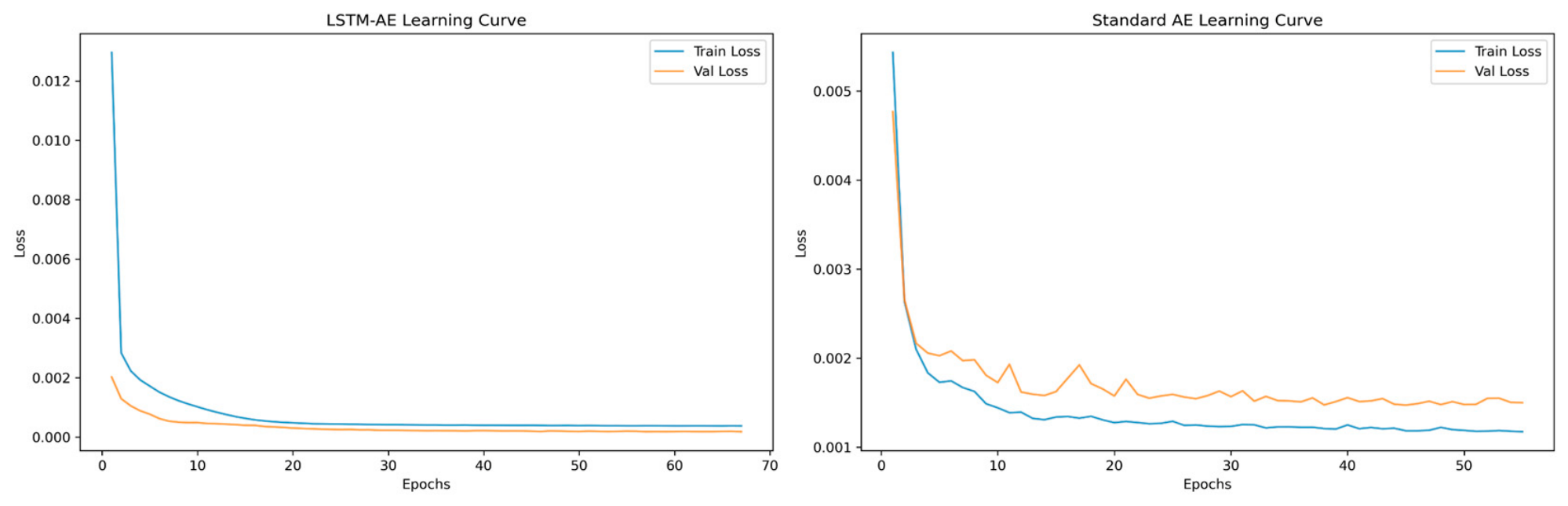
For both phases, the reconstruction loss for the training and validation sets was calculated. The result for both phases is presented in Table 2. The learning curve for phase 2 is shown in Figure 2. The improvement in validation loss from 0.000185 to 0.000179 in phase 2, while numerically small (~3%), is practically significant in power systems as it enables a tighter threshold for anomaly detection, reducing the risk of false positives.

4.2. Anomaly Detection

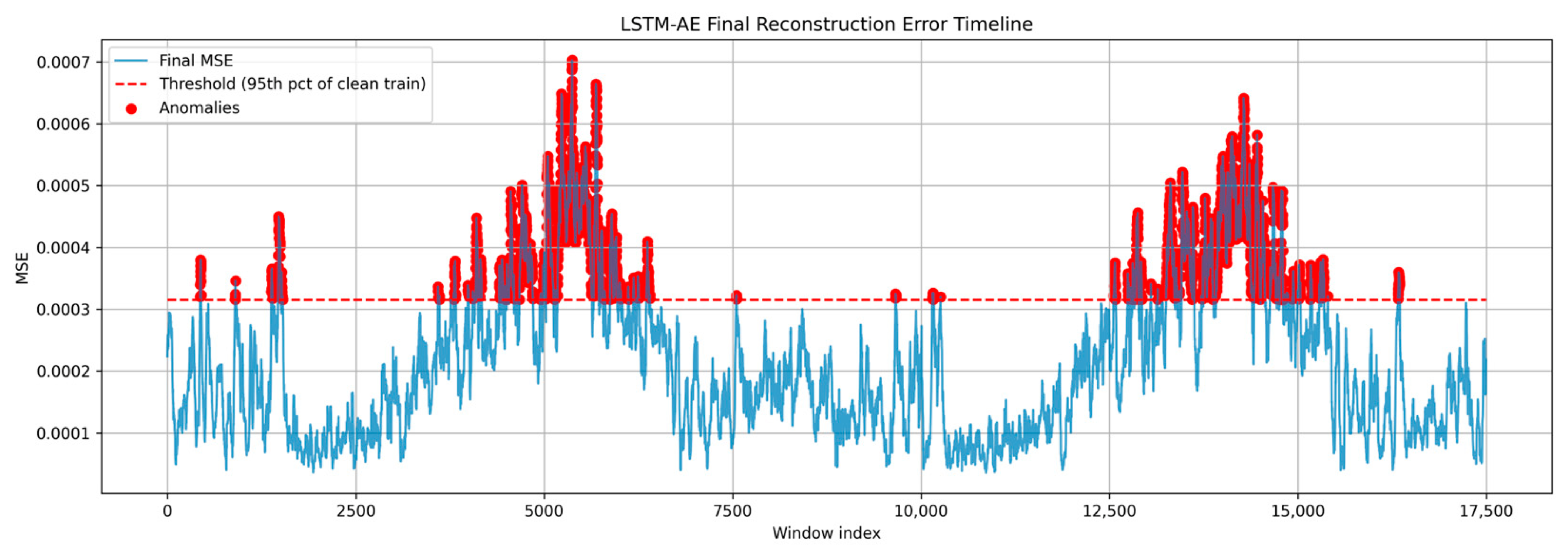
Using the models from the second training phase, an anomaly detection threshold of 95% of all window reconstruction error values was set, corresponding to 0.002315 for the standard autoencoder, and 0.000315 for the LSTM autoencoder. Any window whose reconstruction error exceeded this limit was classified as anomalous. Using this criterion, 3062 and 3501 windows were found to be anomalous for the LSTM autoencoder and standard autoencoder, respectively. A graphical representation of anomalies detected in different windows for the LSTM autoencoder is shown in Figure 3.

4.3. Anomaly Attribution

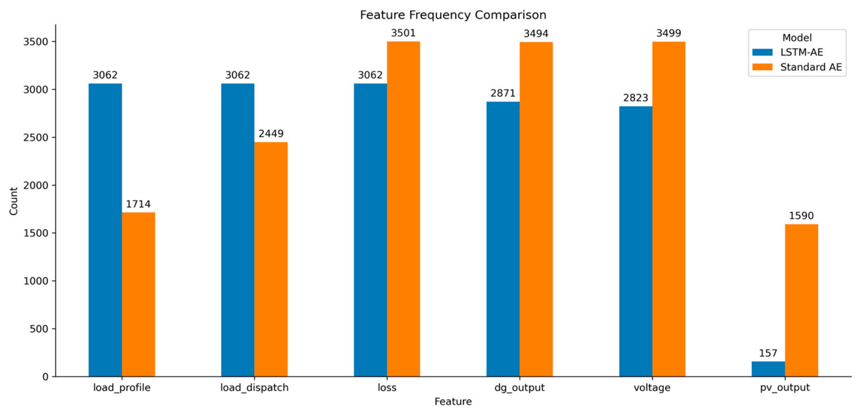
To identify the sources of the detected anomalies, an attribution analysis was done. The analysis of feature importance, as shown in Figure 4, indicates that all the features in the data strongly contributed to the anomalies detected for the LSTM autoencoder, except for pv_output, having only a little influence, while loss, dg_output, and load were the most contributing features for the standard autoencoder.

4.4. Discussion

The results provided several pieces of information on the models’ efficacy and the nature of the anomalies in the dataset. The learning curves for both training phases showed good convergence with consistent decline in both training and validation losses, indicating that the models learned meaningful representations without overfitting. The improved validation loss in the second training phase demonstrates that the refined training process has led to a more accurate and generalized representation of the normal behavior of the system. This is important because it reduces the likelihood of false positives and ensures that model reconstruction errors are a reliable indicator of deviation. The result strongly suggests that the operation of these devices or the events that require their operation are the main factors causing deviations from what the model learnt. This is also confirmed by feature contribution analysis, which identifies loss, dg_output, and load as the main factors for the standard autoencoder, while the LSTM autoencoder captures dependencies across all system variables.

5. Conclusions

This study presents the implementation of a two-stage unsupervised autoencoder framework for power grid time series anomaly detection. The method had an improvement in validation loss in the second stage through statistical filtering of the window with the lowest error. A total of 3062 and 3501 anomalous windows were found for the LSTM and standard autoencoders respectively. The analysis shows that the anomalies found by the standard autoencoder are mainly due to loss, dg_output, and load, while the LSTM-AE detected more dependencies across all variables. These results indicate that reconstruction-based autoencoders achieved better performance for power grid anomaly detection, and they can also provide insights that can help to address targeted monitoring.
Despite this success, there are still some limitations. A fixed 24 h time step window cannot capture anomalies that occur at shorter intervals, like transient faults, or at longer horizons. Future work should focus on using graph neural networks to explicitly model power grid topology. Attention mechanisms can be used to improve readability, with physical constraints to improve data performance. Dynamic threshold adjustment for seasonal patterns, continuous model updates to address conceptual drift, and ensemble techniques to reduce false alarms may also be added.

Author Contributions

Conceptualization, A.O.; methodology, A.O.; software, A.O.; validation, A.O.; formal analysis, A.O.; investigation, A.O.; writing—original draft preparation, A.O.; writing—review and editing, P.O.; visualization, A.O.; supervision, P.O. All authors have read and agreed to the published version of the manuscript.

Funding

This research received no external funding.

Institutional Review Board Statement

Not applicable.

Informed Consent Statement

Not applicable.

Data Availability Statement

Conflicts of Interest

The authors declare no conflicts of interest.

References

  1. Jabbari Zideh, M.; Khushalani Solanki, S. Multivariate physics-informed convolutional autoencoder for anomaly detection in power distribution systems with widespread deployment of distributed energy resources. Sustain. Energy Grids Netw. 2025, 44, 102022. [Google Scholar] [CrossRef]
  2. Powell, J.; McCafferty-Leroux, A.; Hilal, W.; Gadsden, S.A. Smart grids: A comprehensive survey of challenges, industry applications, and future trends. Energy Rep. 2024, 11, 5760–5785. [Google Scholar] [CrossRef]
  3. Hasan, M.K.; Habib, A.A.; Shukur, Z.; Ibrahim, F.; Islam, S.; Razzaque, M.A. Review on cyber-physical and cyber-security system in smart grid: Standards, protocols, constraints, and recommendations. J. Netw. Comput. Appl. 2023, 209, 103540. [Google Scholar] [CrossRef]
  4. Aghazadeh Ardebili, A.; Hasidi, O.; Bendaouia, A.; Khalil, A.; Khalil, S.; Luceri, D.; Longo, A.; Abdelwahed, E.H.; Qassimi, S.; Ficarella, A. Enhancing resilience in complex energy systems through real-time anomaly detection: A systematic literature review. Energy Inform. 2024, 7, 96. [Google Scholar] [CrossRef]
  5. Oyedeji, A.; Olukanmi, P. Intelligent Condition Monitoring of Power Transformers via Machine Learning. In 2025 33rd Southern African Universities Power Engineering Conference (SAUPEC); IEEE: New York, NY, USA, 2025; pp. 1–6. [Google Scholar]
  6. Finke, T.; Krämer, M.; Morandini, A.; Mück, A.; Oleksiyuk, I. Autoencoders for unsupervised anomaly detection in high energy physics. J. High Energy Phys. 2021, 2021, 161. [Google Scholar] [CrossRef]
  7. Ji, T.; Xu, P.; Guo, D.; Sun, L.; Ma, K.; Wang, Y.; Han, X. Variational Autoencoder Based Anomaly Detection in Large-Scale Energy Storage Power Stations. Energies 2025, 18, 2770. [Google Scholar] [CrossRef]
  8. Neloy, A.A.; Turgeon, M. A comprehensive study of auto-encoders for anomaly detection: Efficiency and trade-offs. Mach. Learn. Appl. 2024, 17, 100572. [Google Scholar] [CrossRef]
  9. Sahili, Z.; Al Awad, M. Spatio-Temporal Graph Neural Networks: A Survey. arXiv 2023, arXiv:2301.10569. [Google Scholar] [CrossRef]
  10. Zhang, Y.; Karve, P.M.; Mahadevan, S. Graph neural networks for power grid operational risk assessment under evolving grid topology. arXiv 2024, arXiv:2405.07343. [Google Scholar] [CrossRef]
  11. Cooper, A.; Bretas, A.; Meyn, S. Anomaly Detection in Power System State Estimation: Review and New Directions. Energies 2023, 16, 6678. [Google Scholar] [CrossRef]
  12. Zhang, J.E.; Wu, D.; Boulet, B. Time Series Anomaly Detection for Smart Grids: A Survey. In 2021 IEEE Electrical Power and Energy Conference (EPEC); IEEE: New York, NY, USA, 2021. [Google Scholar]
  13. Yin, T.; Naqvi, S.A.R.; Nandanoori, S.P.; Kundu, S. Advancing Cyber-Attack Detection in Power Systems: A Comparative Study of Machine Learning and Graph Neural Network Approaches. In 2024 Resilience Week (RWS); IEEE: New York, NY, USA, 2024; pp. 1–9. [Google Scholar]
  14. Wei, Y.; Jang-Jaccard, J.; Xu, W.; Sabrina, F.; Camtepe, S.; Boulic, M. LSTM-Autoencoder based Anomaly Detection for Indoor Air Quality Time Series Data. IEEE Sens. J. 2022, 23, 3787–3800. [Google Scholar] [CrossRef]
  15. Hu, D.; Zhang, C.; Yang, T.; Chen, G. Anomaly Detection of Power Plant Equipment Using Long Short-Term Memory Based Autoencoder Neural Network. Sensors 2020, 20, 6164. [Google Scholar] [CrossRef] [PubMed]
  16. Gong, X.; Liao, S.; Hu, F.; Hu, X.; Liu, C. Autoencoder-Based Anomaly Detection for Time Series Data in Complex Systems. In 2022 IEEE Asia Pacific Conference on Circuits and Systems (APCCAS); IEEE: New York, NY, USA, 2022; pp. 428–433. [Google Scholar]
  17. Xu, X.; Qin, F.; Zhao, W.; Xu, D.; Wang, X.; Yang, X. Anomaly Detection with GRU Based Bi-autoencoder for Industrial Multimode Process. Int. J. Control Autom. Syst. 2022, 20, 1827–1840. [Google Scholar] [CrossRef]
  18. Guha, D.; Chatterjee, R.; Sikdar, B. Anomaly Detection Using LSTM-Based Variational Autoencoder in Unsupervised Data in Power Grid. IEEE Syst. J. 2023, 17, 4313–4323. [Google Scholar] [CrossRef]
  19. Lin, R.; Chen, S.; He, Z.; Wu, B.; Zou, H.; Zhao, X.; Li, Q. Electricity Behavior Modeling and Anomaly Detection Services Based on a Deep Variational Autoencoder Network. Energies 2024, 17, 3904. [Google Scholar] [CrossRef]
  20. Shrestha, R.; Mohammadi, M.; Sinaei, S.; Salcines, A.; Pampliega, D.; Clemente, R.; Sanz, A.L.; Nowroozi, E.; Lindgren, A. Anomaly detection based on LSTM and autoencoders using federated learning in smart electric grid. J. Parallel Distrib. Comput. 2024, 193, 104951. [Google Scholar] [CrossRef]
  21. Harrou, F.; Bouyeddou, B.; Dairi, A.; Sun, Y. Exploiting Autoencoder-Based Anomaly Detection to Enhance Cybersecurity in Power Grids. Future Internet 2024, 16, 184. [Google Scholar] [CrossRef]
  22. Park, T.; Song, K.; Jeong, J.; Kim, H. Convolutional Autoencoder-Based Anomaly Detection for Photovoltaic Power Forecasting of Virtual Power Plants. Energies 2023, 16, 5293. [Google Scholar] [CrossRef]
  23. Bank, D.; Koenigstein, N.; Giryes, R. Autoencoders. In Machine Learning for Data Science Handbook: Data Mining and Knowledge Discovery Handbook; Rokach, L., Maimon, O., Shmueli, E., Eds.; Springer International Publishing: Cham, Switzerland, 2023; pp. 353–374. ISBN 978-3-031-24628-9. [Google Scholar]
  24. Lachekhab, F.; Benzaoui, M.; Tadjer, S.A.; Bensmaine, A.; Hamma, H. LSTM-Autoencoder Deep Learning Model for Anomaly Detection in Electric Motor. Energies 2024, 17, 2340. [Google Scholar] [CrossRef]
  25. Son, N.; Jung, M. Analysis of Meteorological Factor Multivariate Models for Medium- and Long-Term Photovoltaic Solar Power Forecasting Using Long Short-Term Memory. Appl. Sci. 2020, 11, 316. [Google Scholar] [CrossRef]
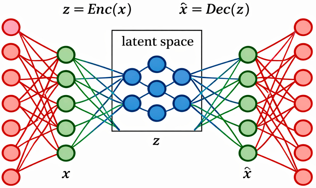
Figure 1. Autoencoder architecture outer and hidden layers represented by the red and green colors.
Engproc 140 00006 g001
Figure 2. Phase 2 learning curve.
Engproc 140 00006 g002
Figure 3. Window timeline showing the MSE, threshold, and anomalous windows for the LSTM autoencoder.
Engproc 140 00006 g003
Figure 4. Feature importance comparison.
Engproc 140 00006 g004
Table 1. Description of the dataset features.
PV OutputLoad ProfileLoad DispatchDG OutputLossVoltageTime Step
Mean0.004110.07890.07220.005880.9950.001568759.500
Std0.01400.09010.08530.02650.02170.003195057.592
Min0.00.00.00.00.95000.00.0
Max0.1200.8400.8360.2501.04950.029717,519.000
Table 2. Validation losses for the two models during each phase.
Training PhaseModel TypeConvergence EpochValidation Loss (MSE)
1Standard AE470.001515
1LSTM-AE890.000185
2Standard AE450.001472
2LSTM-AE570.000179
Disclaimer/Publisher’s Note: The statements, opinions and data contained in all publications are solely those of the individual author(s) and contributor(s) and not of MDPI and/or the editor(s). MDPI and/or the editor(s) disclaim responsibility for any injury to people or property resulting from any ideas, methods, instructions or products referred to in the content.