Proceeding Paper

Scheduling Solar-Dryer Operating Windows from Learned Drying Rate Trajectories †
by
Niño Louie R. Boloron
1,2,*,
Karell Keith P. Gulben
1,
Datu Al-Ashari Salat
1 and
Basilio Corleone U. Boddie
1
1
Mechanical Engineering Department, College of Engineering and Architecture, Mapua Malayan Colleges Mindanao, Davao City 8000, Davao del Sur, Philippines
2
Mechanical Engineering Department, College of Engineering, Central Mindanao University, Maramag 8710, Bukidnon, Philippines
*
Author to whom correspondence should be addressed.
Presented at the 7th Eurasia Conference on IoT, Communication and Engineering 2025 (ECICE 2025), Yunlin, Taiwan, 14–16 November 2025.
Eng. Proc. 2026, 134(1), 100; https://doi.org/10.3390/engproc2026134100
Published: 14 July 2026

Abstract

We developed a telemetry-driven scheduler that recommends hour-by-hour operating windows for a small solar dryer used for Moro-Moro fish. Operational logs and moisture-ratio (MR) trajectories are aligned with solar resource descriptors and chamber thermal states to learn MR decline as a function of elapsed time and conditions. A nonparametric tree-based trajectory learner generates point forecasts of MR and, in parallel, uncertainty intervals obtained through quantile regression and conformal calibration. Schedules are synthesized by projecting the time-to-threshold (e.g., MR ≤ 0.20) under the learned trajectories and selecting operating windows that minimize completion time while enforcing uncertainty-aware guardrails. Using the project’s DRYER telemetry, a cold-start model captures typical drying curves from historical runs, while an online (recursive) variant adapts within a run as new MR observations arrive. The approach yields accurate held-out predictions, empirically reasonable interval coverage given the limited sample, and transparent schedules that can be printed or sent as JSON payloads for operators. The pipeline is robust to short telemetry gaps through conservative imputation policies and incorporates a chamber “health” index that flags regime shifts before schedules degrade.

1. Introduction

Solar drying is widely used to preserve fish and other high-moisture food products in coastal communities, yet traditional open-sun drying remains vulnerable to contamination, weather variability, and inconsistent product quality. Recent reviews emphasize that modern solar dryers, with controlled airflow, enclosed chambers, and tailored heat-transfer configurations, can substantially improve efficiency and hygiene compared with open-sun practices [1]. Thin-layer drying models have been extensively applied to characterize agricultural product drying in solar systems, providing generalized drying curves and time estimates but typically assuming stable laboratory conditions and dense measurements that may not hold in field deployments [2].
In practice, small-scale dryers in coastal communities operate under nonstationary, data-scarce conditions: sensors fail intermittently, weather shifts rapidly, and local operators cannot continuously monitor trajectories. Surveys on missing data in machine learning highlight how naïve imputation can bias downstream models and emphasize the need for structure-aware handling in time-series settings [3]. At the same time, interpretability remains crucial when embedding machine learning into operational decisions. Tree-based Shapley Additive Explanations (TreeSHAP) provides consistent, individualized feature attributions for tree ensembles and is widely used to explain gradient-boosted models [4]. Offline change-point detection and time-series feature engineering methods provide tools for identifying regime shifts and constructing informative temporal features, which are especially important in multi-run experimental data [5,6]. Probabilistic forecasting with quantile regression has become standard in renewable-energy and building-load applications, allowing models to output conditional quantiles rather than point forecasts [7]. Conformal prediction adds distribution-free uncertainty quantification with finite-sample guarantees [8], and conformalized quantile regression (CQR) combines conformal prediction with classical quantile regression to obtain adaptive prediction intervals [9]. Gradient-boosted decision trees, such as Light Gradient Boosting Machine (LightGBM), are widely adopted for tabular energy and engineering problems due to their accuracy and efficiency [10], and recent work demonstrates that conformal and CQR-style approaches can provide calibrated prediction intervals for load and energy forecasting tasks [11].
From the predict-then-optimize perspective, forecasting quality must be evaluated by the downstream decisions it supports, rather than by error metrics alone [12]. Building on these ideas, we developed a conformalized quantile gradient boosting (CQGB) framework for risk-aware drying-schedule synthesis in a small solar-assisted fish dryer, integrating robust preprocessing, calibrated probabilistic forecasting, a health index, and simple policies that explicitly trade off drying time against the risk of under- and over-drying.

2. Methodology

2.1. Dataset

In the case study, we used telemetry from a mixed-mode solar dryer with auxiliary nichrome-wire heating designed for Moro-Moro fish in Davao City, Philippines. Each drying run corresponds to a batch of prepared fillets loaded onto trays inside the drying chamber. During operation, ambient temperature and humidity, chamber air temperature and humidity, heater status, and product mass are recorded at regular intervals; initial moisture content is determined at loading. From the mass measurements and initial moisture, we derive the moisture ratio (MR), defined as the ratio of current to initial moisture content, which serves as the primary response variable. Runs were conducted across a range of weather conditions and loading configurations, so the resulting dataset covers both favorable sunny days and marginal conditions with clouds or high ambient humidity.
The raw time series contains gaps and occasional anomalies due to sensor dropouts and communication issues. After cleaning and time-alignment, we obtain a set of run-level time series, where each record is a snapshot containing the current MR, environmental, and chamber conditions, the heater state, and derived temporal features. Figure 1 illustrates representative MR trajectories from several experimental runs, highlighting how drying rates vary with ambient conditions and heater usage. On favorable days, MR declines smoothly toward the target safe moisture band within a relatively short time window, while on marginal days, MR decays slowly and may remain near or above the safety threshold well into the afternoon. These observed patterns motivate the need for a forecasting and scheduling framework that accounts for uncertainty and variability across runs, rather than relying on fixed-time heuristics.

2.2. Trajectory Learner

The predictive component is a gradient-boosted decision-tree ensemble implemented in LightGBM. We train (i) a point model for MR and (ii) quantile models for uncertainty bounds. To ensure a leak-free cold-start formulation, the cold-start model uses only exogenous and time-derived predictors that are available at the start of a run, namely elapsed time since loading (time_min, time_hr), time-of-day harmonics (hour_sin, hour_cos), available environmental drivers (e.g., temperature, relative humidity, and irradiance when present), and a categorical policy indicator. The resulting cold-start model directly maps these predictors to MR, enabling it to generate an expected drying trajectory as a function of elapsed time under the observed conditions.
Because MR is expected to decrease as drying progresses, we apply monotonic constraints on elapsed time to the point model. Quantile models (P10, P50, P90) are trained under LightGBM’s quantile objective and are used to form raw prediction bands; due to objective-level constraints in LightGBM, monotonic constraints are applied to the point model but not enforced in the quantile objective. Predictions are finally clipped to the physically meaningful range MR ∈ [0, 1].

2.3. Cold-Start and Online Updating

To support both pre-run planning and within-run adaptation, we distinguish between a cold-start (CS) model and an online model. The CS variant is trained exclusively on completed historical runs and is used at the start of a new batch when no current-run MR observations have been recorded. It encodes prior knowledge about typical drying trajectories as a function of weather, loading time, and initial chamber conditions. Once the run begins and a few MR measurements become available, the online model continually refines forecasts by conditioning on the observed trajectory so far.
In practice, the online variant starts from the CS model parameters and is updated walk-forward. At each step, the model processes data from past time steps and earlier runs. This protocol mimics deployment, in which future information is unavailable when making predictions. The CS model provides initial estimates of time-to-safe-moisture that are useful for planning, whereas the online model corrects for day-specific deviations such as unusually high humidity or atypical loading patterns. The two modes allow the scheduler to provide early guidance at loading time and increasingly precise recommendations as drying progresses.

2.4. Uncertainty Quantification

Quantile regression directly estimates conditional quantiles of MR at each horizon, but the resulting prediction intervals can be miscalibrated in finite samples or under model misspecification [7]. To obtain finite-sample, distribution-free marginal coverage under an exchangeability assumption, we wrap the LightGBM quantile model in conformalized quantile regression (CQR) [9]. Drying runs are split into three disjoint subsets at the run level: a training set used to fit the quantile model, a calibration set used to adjust intervals, and a test set used solely for evaluation. After training, we compute nonconformity scores on the calibration set as the maximum deviation of each observation from the predicted lower and upper quantiles at each time step, and use the empirical quantiles of these scores to form an additive inflation term that widens the raw quantile band to the desired nominal level.
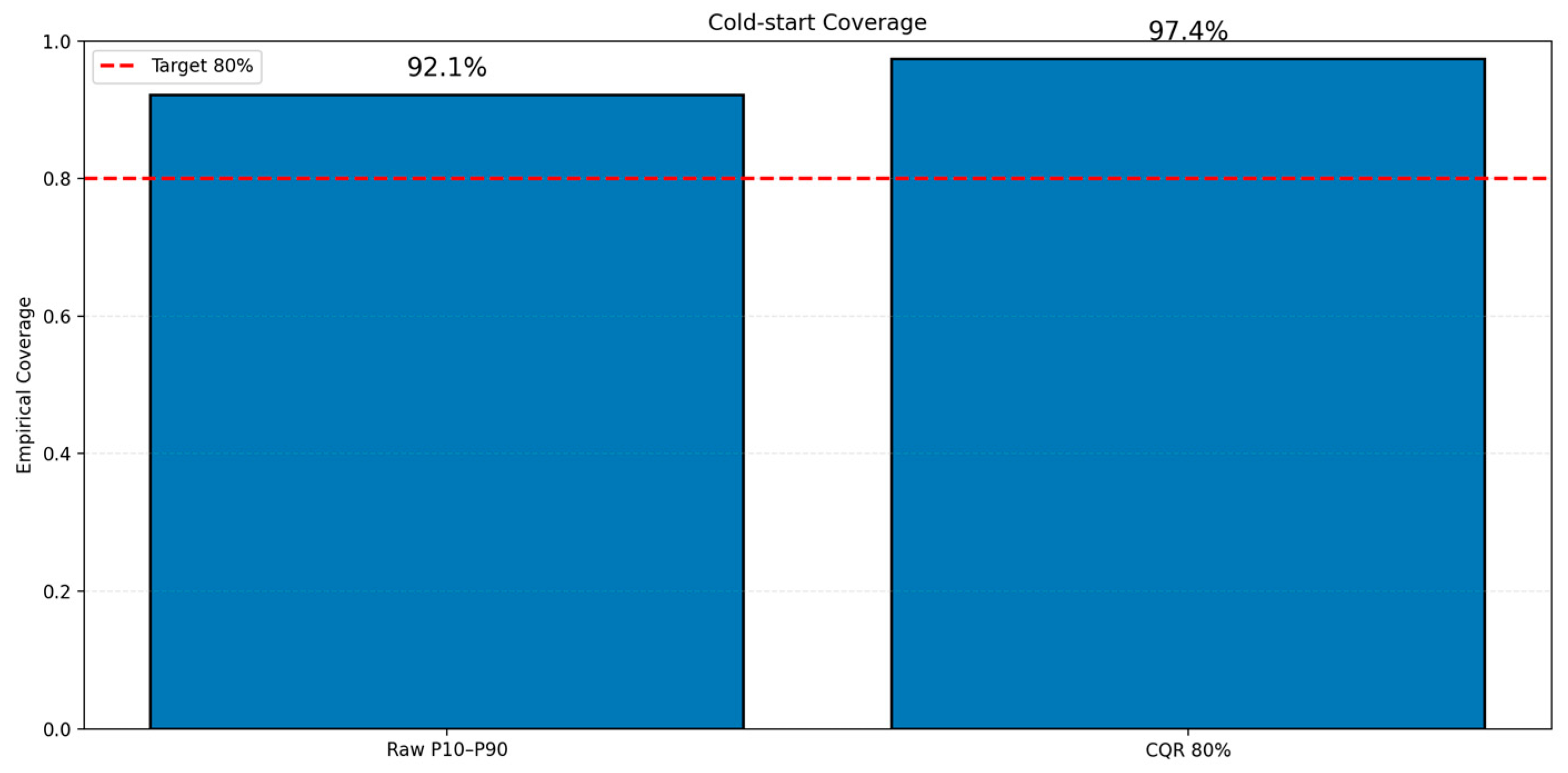
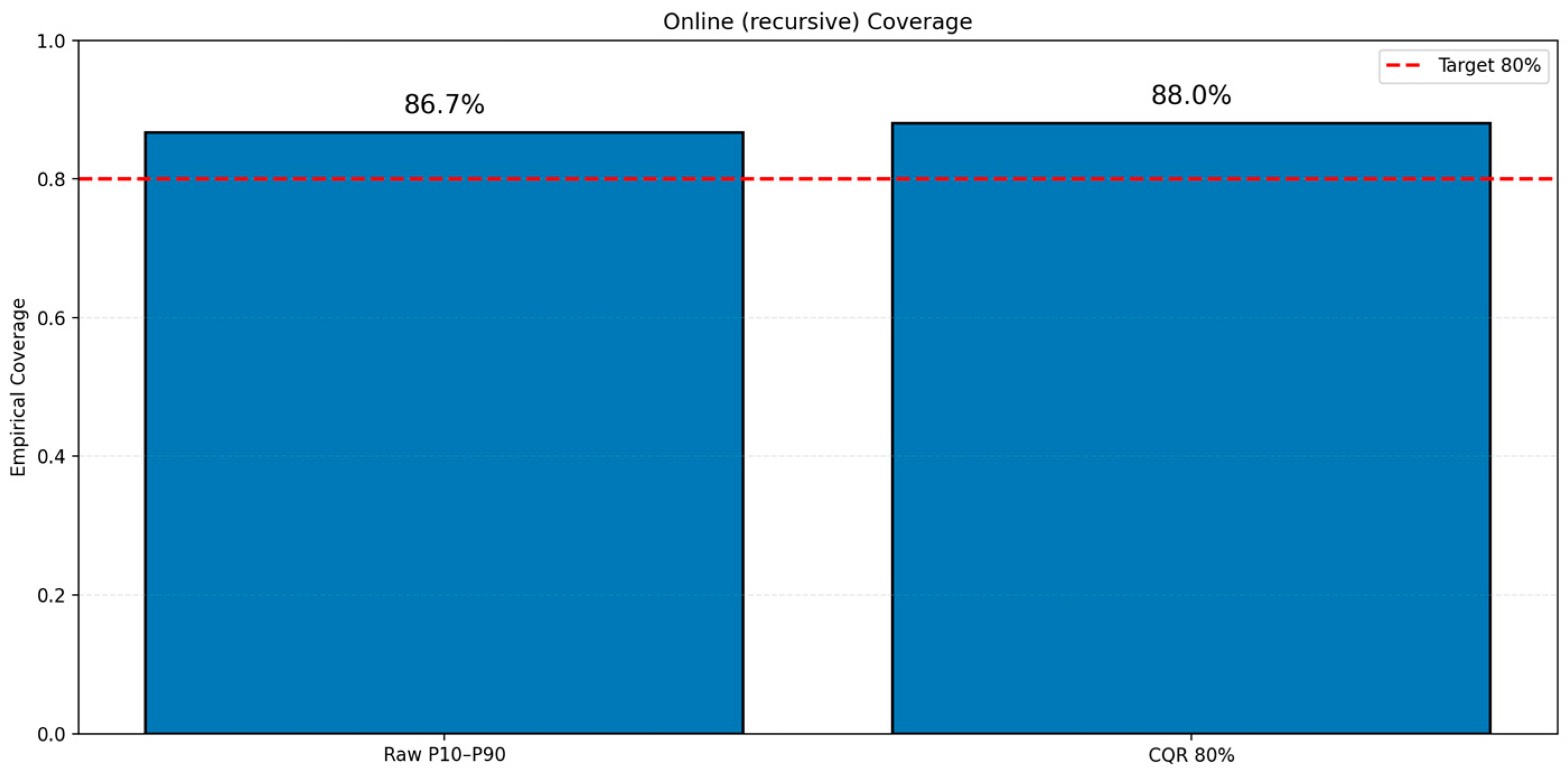
In this dataset, the raw P10–P90 bands are already conservative on held-out runs, and CQR therefore acts primarily as an additional safety margin rather than a correction for pronounced under-coverage. At the 80% nominal level, cold-start coverage increases from 92.1% (raw) to 97.4% (CQR), while online coverage increases from 86.7% (raw) to 88.0% (CQR) (Figure 2 and Figure 3; Table 1). The corresponding conformal inflation terms are small (CS_qhat = 0.0061; ON_qhat = 0.0041), consistent with relatively tight but conservative uncertainty bands for a bounded target MR ∈ [0, 1].

2.5. Schedule Synthesis and Guardrails

We translate probabilistic MR trajectories and their conformalized intervals into drying schedules by defining simple decision policies that map forecasts to start/stop rules. A risk-neutral policy continues drying until the median forecasted MR is projected to fall below the upper safety threshold within a short future window, then terminates the run. A conservative policy in contrast, requires that the upper conformal bound fall below the safety threshold over a longer window, thereby greatly reducing the probability that the true MR remains unsafe at termination. A third, flexible policy behaves conservatively when the intervals are wide, or the median forecast is close to the threshold, but switches to a more aggressive stopping rule when the intervals tighten, and MR is predicted to enter the safe band quickly.
Each policy can be encoded as a set of guardrails on forecasted quantiles and interval widths. We simulate these policies across historical runs by stepping through each run in time, querying the CQGB forecasts and intervals, and applying the corresponding stop conditions. For each simulated schedule, we record the completion time, the MR trajectory at termination, and the resulting health index summaries. The simulation outputs are aggregated into tables and plots that show how completion time and risk trade off under different policy choices. This “predict-then-optimize” design directly links forecast properties to decisions and aligns with recent work on learning models evaluated by downstream optimization performance [12].

2.6. Health Index and Regime-Shift Flags

To connect MR forecasts to safety and quality outcomes, we define a scalar health index (HI) that penalizes deviations from a target safe moisture band. At each time step, HI accumulates penalties for under-drying when MR exceeds an upper safety threshold associated with microbial risk, and for over-drying when MR drops below a lower threshold associated with quality loss and unnecessary energy use. The penalty weights are selected in consultation with local stakeholders to reflect their relative aversion to under- versus over-drying, but the construction itself is generic and can be adapted to other products or risk preferences.
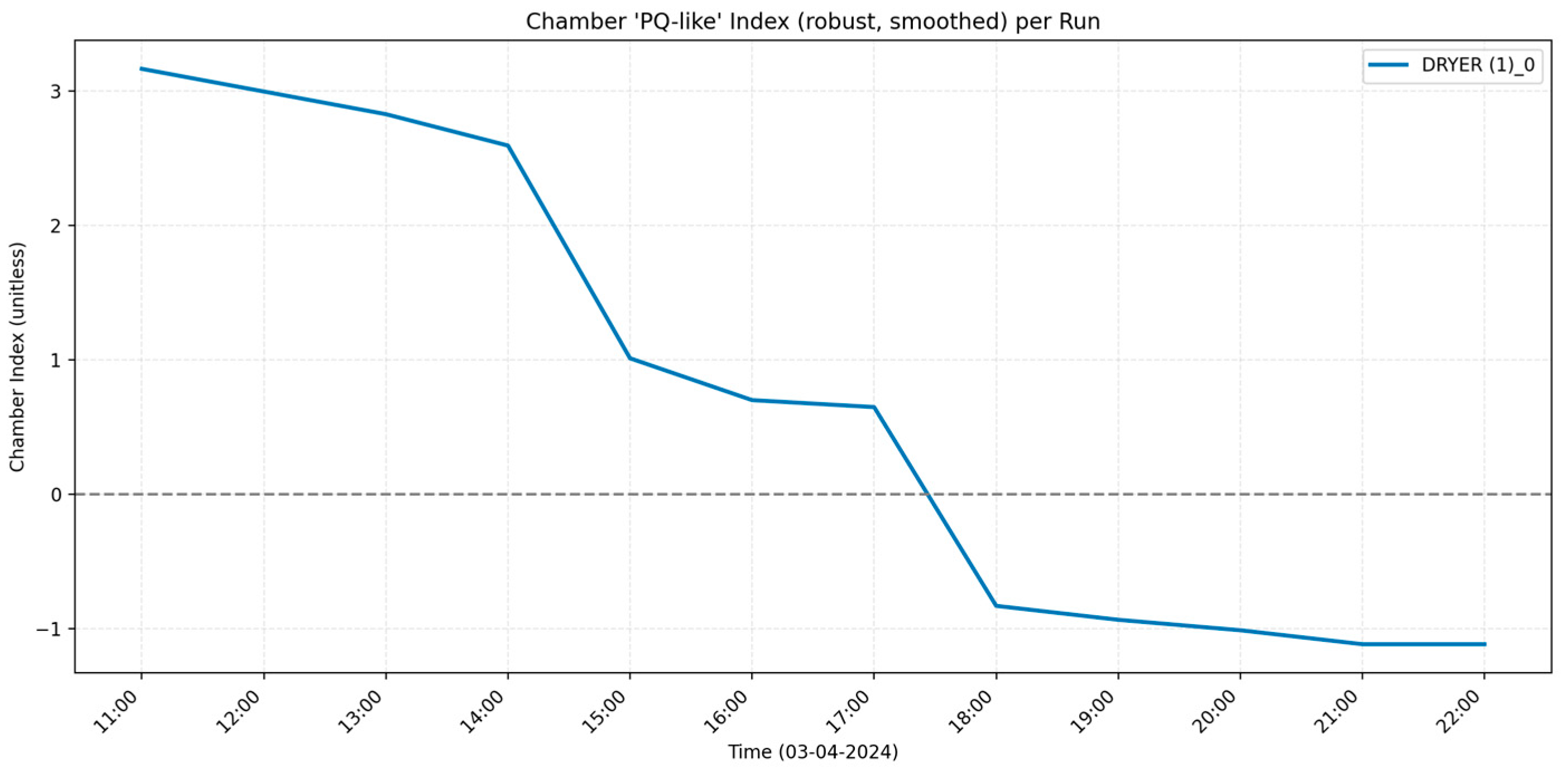
Using the CQGB forecasts and conformal intervals, we compute expected HI trajectories and summary statistics such as peak HI and area under the HI curve for each run and policy. Figure 4 illustrates HI trajectories for representative under-dried, well-dried, and over-dried runs: under-dried runs show sustained high HI values, well-dried runs slope smoothly toward zero as MR enters the safe band, and over-dried runs exhibit extended periods near zero MR with quality-penalty contributions. In addition, we derive simple regime-shift flags from changes in MR gradients and thermal variables, inspired by offline change-point detection methods [5]. These flags identify time segments where drying behavior changes abruptly—such as when weather fronts move in or airflow patterns shift—and can be used to trigger more conservative policies or operator inspections when needed.

2.7. Explainability and Diagnostics

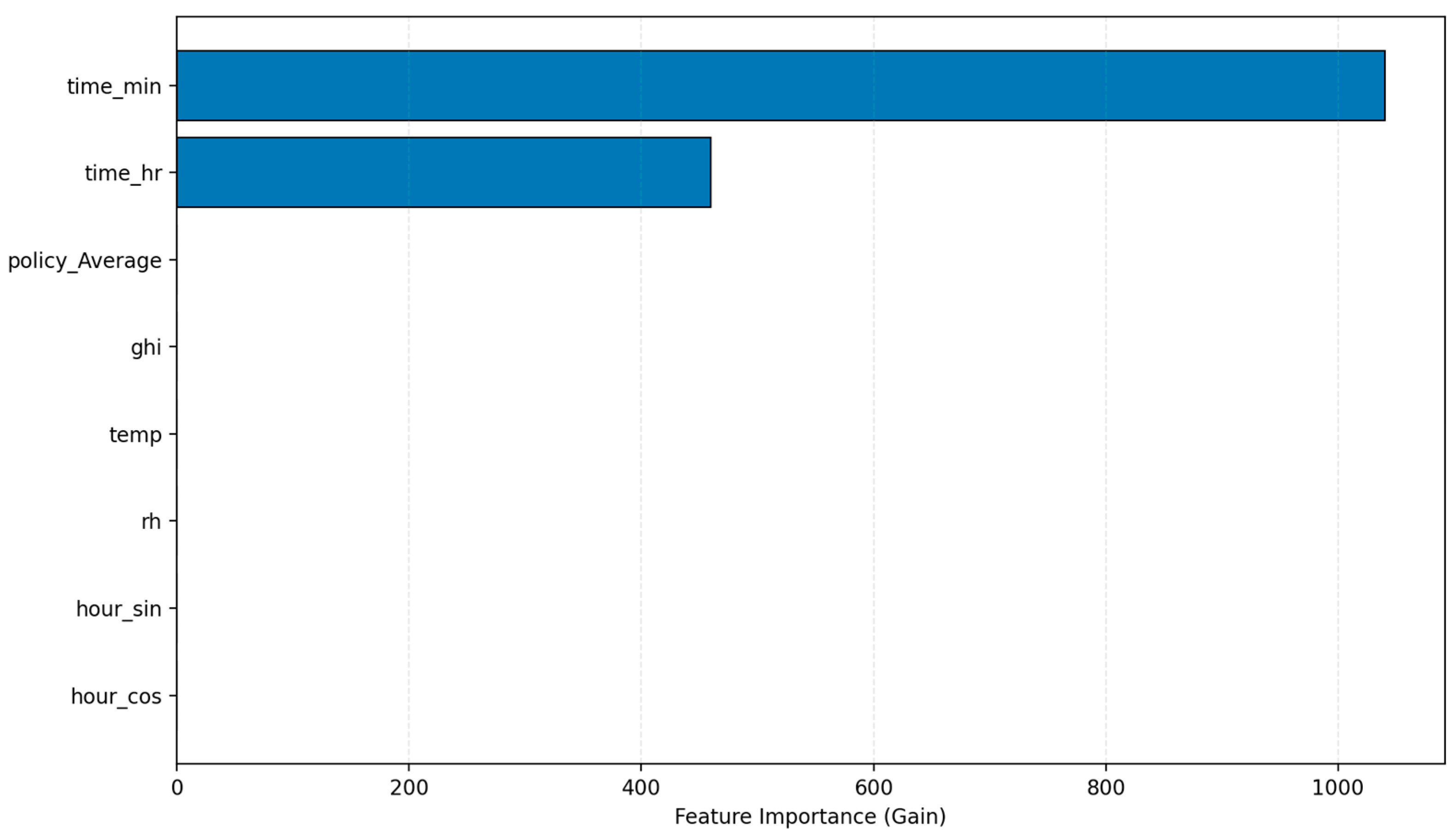
To make the CQGB model interpretable to operators and engineers, we apply TreeSHAP to compute individualized feature attributions for each forecast [4]. Global SHAP summaries (Figure 5) indicate that recent MR, chamber temperature, heater status, and ambient humidity are the most influential features across horizons. Time-of-day indicators and regime-shift flags become more important at longer horizons, reflecting their ability to capture diurnal patterns and structural changes in drying behavior. These patterns align with physical intuition: the current moisture state and internal thermal environment strongly shape drying rate, while ambient humidity and detected change points help adjust expectations under evolving conditions.
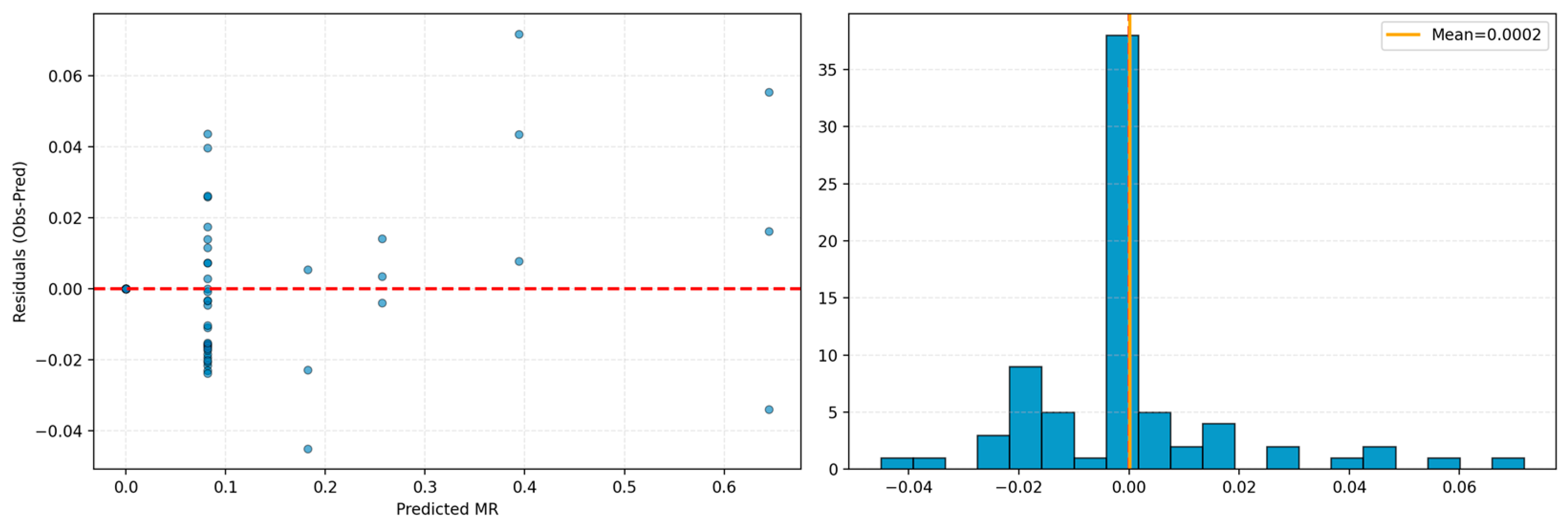
Residual diagnostics complement the SHAP analysis. Figure 5 presents a residual scatter plot and distribution histogram for the cold-start CQGB forecasts on 76 held-out test observations, where each point represents a single observation plotted against its predicted MR value and the dashed red line marks zero residual, indicating perfect agreement between observed and predicted values; points above the line reflect under-prediction and points below reflect over-prediction. The histogram on the right summarizes the distribution of these residuals, with the orange vertical line marking the mean residual of 0.0022, confirming negligible systematic bias across the test set. The residual distribution exhibits a standard deviation of 0.0216, strong positive skewness of 1.9870, and excess kurtosis of 5.8326, indicating that while the majority of errors are small and tightly centered near zero—with 59.2% of test observations falling within ±0.01 MR and 94.7% within ±0.05 MR—a modest proportion of observations produce larger positive errors, reflecting a right-skewed tail. Phase-wise decomposition reveals an important heteroscedastic pattern: the late drying phase (MR ≤ 0.20, n = 67) exhibits the tightest residuals (mean = −0.0024, std = 0.0139), reflecting the model’s strongest predictive accuracy precisely where scheduling decisions—such as determining the end of the drying window—matter most. The mid phase (0.20 < MR ≤ 0.60, n = 6) and early phase (MR > 0.60, n = 3) show wider residual spreads (std = 0.0302 and std = 0.0366 respectively), though both phases are represented by few test samples and their statistics should be interpreted cautiously. Six observations (7.9% of the test set) were identified as outliers with residuals exceeding 2 standard deviations, concentrated in the predicted MR range [0.0821, 0.6043], spanning the mid- and late-phase boundary. The absence of strong systematic bias across drying phases supports the exchangeability assumption underlying the conformal quantile regression framework, and the observed heteroscedasticity in the early and mid phases justifies the use of adaptive interval widths, as conformalized intervals automatically widen in these higher-uncertainty regions. Operationally, practitioners can rely on model predictions with the greatest confidence during the final drying phase, while the wider prediction intervals in the early and mid phases serve as an automatic signal to exercise greater caution or increase monitoring frequency during those periods.

2.8. Pre-Processing, Missingness, and Splits

Pre-processing aligns each drying run to a common time base measured from the start of loading. Moisture ratio (MR) is computed from the available mass and moisture measurements and restricted to the physically meaningful interval [0, 1]. Runs are segmented using time-gap rules so that all observations within a run correspond to a single batch under a shared operating context.
Environmental covariates (e.g., temperature, relative humidity, and irradiance when available) are converted to numeric form, and missing values are imputed using within-run robust summaries to avoid injecting information across runs. Time features (elapsed time and time-of-day harmonics) are computed deterministically from timestamps, and categorical policy labels are encoded as indicator variables.
To evaluate performance on unseen runs, training, calibration, and test sets are defined at the run level (not the time-step level), ensuring that all records from a given run appear in only one split. We use a balanced run-wise splitting strategy that targets approximately a 60/20/20 partition by record count while preserving run integrity. Conformal calibration is computed on the calibration split only, and all metrics and plots in Section 3 are reported exclusively on the held-out test split.

2.9. Evaluation Metrics and Artifacts

We assess point forecasts using mean absolute error (MAE), root mean squared error (RMSE), and coefficient of determination (R2) over held-out time-step predictions from test runs. Interval quality is evaluated via empirical coverage of nominal-level prediction intervals, comparing the raw quantile band (P10–P90) against conformalized quantile regression (CQR) at the 80% nominal level. Table 1 summarizes leak-free metrics for both cold-start and online configurations.
Beyond aggregate metrics, the pipeline produces artifacts that support interpretation and deployment. These include time-to-threshold estimates (τ summaries) and schedule tables listing recommended operating windows under different risk stances (Table 2), along with empirical coverage comparisons (Figure 2 and Figure 3), feature-importance summaries (Figure 5), residual diagnostics (Figure 6), and diagnostic plots such as goodness-of-fit scatter plots (Figure 7 and Figure 8). Together, these artifacts provide an operationally relevant view of both accuracy and risk.

3. Results and Discussion

3.1. Accuracy on Held-Out Runs

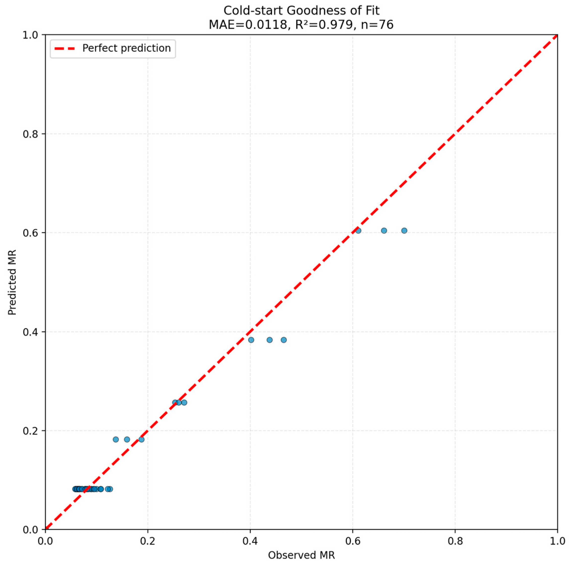
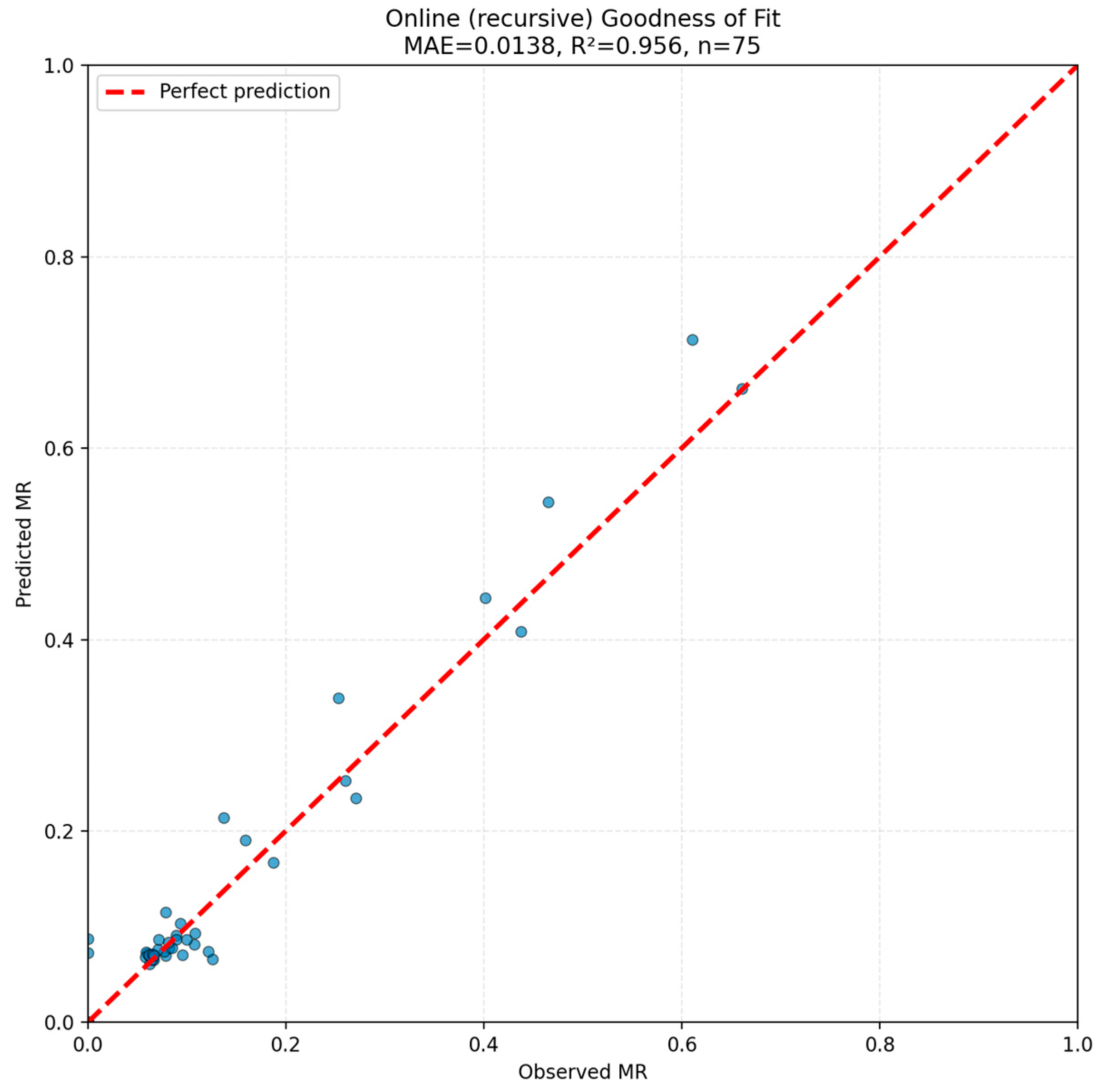
On held-out runs, the CQGB model shows strong agreement between predicted and observed moisture ratio (MR) in both evaluation modes. In the cold-start setting (Figure 7), predictions closely track the 1:1 line with MAE = 0.0118, RMSE = 0.0218, and R2 = 0.9790 over n = 76 samples, indicating that the learned trajectories reproduce the overall scale and shape of drying behavior without run-specific adaptation. In the online (recursive) setting (Figure 8), performance remains high with MAE = 0.0138, RMSE = 0.0279, and R2 = 0.9564 over n = 75 samples, consistent with modest degradation from recursive multi-step prediction and day-specific deviations that are only partially explained by limited within-run observations.
Dispersion increases as MR approaches very low values, where small absolute deviations become visually amplified; however, this tail region is less consequential for under-drying risk than the mid-trajectory regime near the safety threshold. Together with the summary metrics in Table 1, these goodness-of-fit results support using CQGB forecasts as the predictive backbone for schedule synthesis, provided uncertainty intervals are carried into decision rules when operating close to the threshold.

3.2. Interval Calibration

Interval calibration is evaluated by empirical coverage of the nominal 80% prediction interval, comparing raw quantile bands (P10–P90) against conformalized quantile regression (CQR). In the cold-start configuration (Figure 2), the raw P10–P90 interval already over-covers at 92.1%, and CQR further increases coverage to 97.4%. In the online configuration (Figure 3), raw coverage is 86.7% and increases to 88.0% after CQR. This indicates that the base quantile models are conservative in this dataset, and that conformalization primarily adds a safety margin rather than correcting severe under-coverage.
Formally, letting q ^ l o x and q ^ h i x denote the predicted lower and upper quantiles, the CQR nonconformity score on a calibration sample x i , y i is s i = m a x q ^ l o x i y i ,   y i q ^ h i x i , 0 , which is nonnegative by construction. The conformal inflation term is q ^ = Q u a n t i l e 1 α s i , yielding calibrated intervals q ^ l o x q ^ ,   q ^ h i x + q ^ . In Table 1, q ^ is small and positive (CS_qhat = 0.0061; ON_qhat = 0.0041), consistent with conservative but relatively tight intervals given the bounded MR target and the limited number of calibration samples.

3.3. Operational Value

Simulated application of the scheduling policies shows clear trade-offs between drying time and risk. Under the risk-neutral policy, many runs terminate relatively early, and MR at termination is typically within or just below the target safe band; however, when ambient humidity remains high or clouds persist, the upper conformal bound can still overlap the safety threshold at the chosen stop time, leaving a non-negligible probability of under-drying. The conservative policy, by contrast, requires that the entire conformal interval lies within the safe band over a future window, substantially reducing under-drying risk at the cost of longer average completion times. HI trajectories under this policy (Figure 4) converge smoothly toward zero and exhibit few late-run excursions, indicating robust safety margins.
The flexible policy balances these extremes by adapting to the width and position of the conformal intervals. When forecasts are tight, and MR is projected to enter the safe band quickly, the policy behaves similarly to the risk-neutral rule, enabling earlier termination. When intervals are wide or uncertain, the policy reverts to conservative guardrails, extending drying until high-confidence safety conditions are met. Table 2 summarizes completion times and HI outcomes under all three policies: the flexible policy recovers much of the time savings of the risk-neutral strategy while maintaining health-index profiles close to those of the conservative policy. Table 2 illustrates representative completion windows for three runs; a fuller set of run-level schedules is omitted for brevity. For small-scale operators, this suggests a practical interface that presents a small menu of labeled policies (faster but riskier, balanced, and slow but safest) along with expected completion times and risk summaries, thereby embedding sophisticated, uncertainty-aware optimization into simple, interpretable choices.

4. Conclusions

We developed a risk-aware drying schedule synthesis framework for a small-scale solar-assisted fish dryer by integrating conformalized quantile gradient boosting with a health index and simple decision policies. The framework combines structure-aware preprocessing, time-series feature engineering, and LightGBM-based quantile modeling to generate moisture-ratio forecasts with calibrated uncertainty estimates. TreeSHAP analysis results confirmed that the model relies on physically meaningful predictors, including recent MR, chamber temperature, heater status, and ambient humidity. The derived HI and policy simulations translated these probabilistic forecasts into actionable drying schedules that explicitly balance completion time against the risks of under- or over-drying. An adaptive policy can recover much of the time savings associated with a risk-neutral strategy while preserving the safety and quality benefits of a conservative approach. These results illustrate how uncertainty-aware machine learning can enhance the safe and efficient operation of small-scale post-harvest technologies in data-scarce and variable environments, while motivating future work on broader experimental validation, richer quality indicators, and lightweight interfaces that present forecast and risk information in accessible formats for local operators.

Author Contributions

Conceptualization, N.L.R.B.; methodology, N.L.R.B., K.K.P.G., D.A.-A.S. and B.C.U.B.; validation, N.L.R.B.; formal analysis, N.L.R.B.; investigation, K.K.P.G., D.A.-A.S. and B.C.U.B.; data curation, N.L.R.B., K.K.P.G., D.A.-A.S. and B.C.U.B.; writing—original draft preparation, N.L.R.B., K.K.P.G., D.A.-A.S. and B.C.U.B.; writing—review and editing, N.L.R.B.; visualization, N.L.R.B.; supervision, N.L.R.B. All authors have read and agreed to the published version of the manuscript.

Funding

This research was funded purely by the proponents. Mapua Malayan Colleges Mindanao provided financial support for participation in the conference and for the presentation of the paper.

Institutional Review Board Statement

Not applicable. This study did not involve human participants, human biological materials, animals, or personally identifiable human-subject data.

Informed Consent Statement

Not applicable.

Data Availability Statement

The data presented in this study are available from the corresponding author upon reasonable request and subject to the removal of security-sensitive facility information.

Acknowledgments

Gratitude is extended to Mapua Malayan Colleges Mindanao for sharing the resources and equipment needed to conduct the research.

Conflicts of Interest

The authors declare no conflicts of interest.

References

  1. Fernandes, L.; Tavares, P.B. A review on solar drying devices: Heat transfer, air movement and type of chambers. Solar 2024, 4, 15–42. [Google Scholar] [CrossRef] [Scilit]
  2. Kidane, H.; Farkas, I.; Buzás, J. Characterizing agricultural product drying in solar systems using thin-layer drying models: Comprehensive review. Discov. Food 2025, 5, 84. [Google Scholar] [CrossRef] [Scilit]
  3. Emmanuel, T.; Maupong, T.; Mpoeleng, D.; Semong, T.; Mphago, B.; Tabona, O. A survey on missing data in machine learning. J. Big Data 2021, 8, 140. [Google Scholar] [CrossRef] [Scilit] [PubMed]
  4. Lundberg, S.M.; Erion, G.G.; Lee, S.-I. Consistent individualized feature attribution for tree ensembles. arXiv 2018, arXiv:1802.03888. [Google Scholar]
  5. Truong, C.; Oudre, L.; Vayatis, N. Selective review of offline change point detection methods. Signal Process. 2020, 167, 107299. [Google Scholar] [CrossRef] [Scilit]
  6. Wang, C.; Baratchi, M.; Bäck, T.; Hoos, H.H.; Limmer, S.; Olhofer, M. Towards time-series feature engineering in automated machine learning for multi-step-ahead forecasting. Eng. Proc. 2022, 18, 17. [Google Scholar] [CrossRef]
  7. Xu, C.; Sun, Y.; Du, A.; Gao, D.-C. Quantile regression based probabilistic forecasting of renewable energy generation and building electrical load: A state of the art review. J. Build. Eng. 2023, 79, 107772. [Google Scholar] [CrossRef] [Scilit]
  8. Angelopoulos, A.N.; Bates, S. A gentle introduction to conformal prediction and distribution-free uncertainty quantification. arXiv 2021, arXiv:2107.07511. [Google Scholar]
  9. Romano, Y.; Patterson, E.; Candès, E.J. Conformalized quantile regression. In Proceedings of the 33rd Conference on Neural Information Processing Systems (NeurIPS 2019), Vancouver, BC, Canada, 8–14 December 2019; Curran Associates Inc.: Red Hook, NY, USA, 2019; pp. 3538–3548. [Google Scholar]
  10. Ke, G.; Meng, Q.; Finley, T.; Wang, T.; Chen, W.; Ma, W.; Ye, Q.; Liu, T.-Y. LightGBM: A highly efficient gradient boosting decision tree. In Proceedings of the 31st Conference on Neural Information Processing Systems (NIPS 2017), Long Beach, CA, USA, 4–9 December 2017; Curran Associates Inc.: Red Hook, NY, USA, 2017; pp. 3146–3154. [Google Scholar]
  11. Matulin, L.; Capuder, T.; Plavšić, T. Short-term probabilistic load forecasting based on conformalized quantile regression. In Proceedings of the 15th International Conference on Applied Energy (ICAE 2023), Doha, Qatar, 3–7 December 2023. [Google Scholar]
  12. Elmachtoub, A.N.; Grigas, P. Smart “Predict, then Optimize”. Manag. Sci. 2022, 68, 9–26. [Google Scholar] [CrossRef] [Scilit]
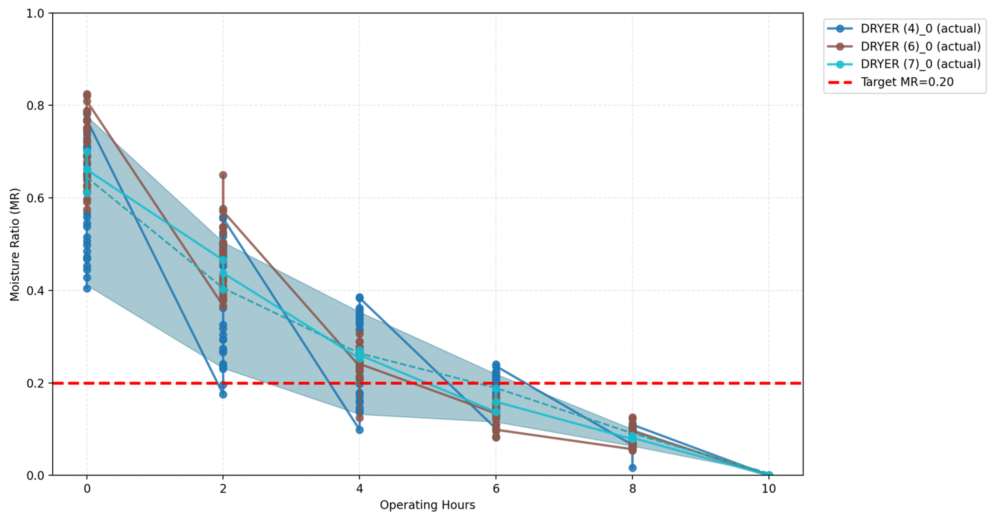
Figure 1. Learned drying rate (MR) trajectories.
Engproc 134 00100 g001
Figure 2. Cold-start empirical interval coverage and 80% target.
Engproc 134 00100 g002
Figure 3. Online empirical interval coverage and 80% target.
Engproc 134 00100 g003
Figure 4. Chamber HI (robust, smoothed) per run.
Engproc 134 00100 g004
Figure 5. Most influential trajectory descriptors (cold-start): model-reported feature importance (gain).
Engproc 134 00100 g005
Figure 6. Residual diagnostics: residuals vs. fitted (left) and residual distribution with mean and standard deviation (right). In the scatter plot, each point represents a single held-out observation plotted against its predicted MR value, and the dashed red line marks zero residual; points above the line indicate under-prediction and points below indicate over-prediction. The histogram summarizes the residual distribution across 76 test observations, with the orange vertical line marking the mean residual of 0.0022.
Engproc 134 00100 g006
Figure 7. Cold-start goodness-of-fit: predicted vs. observed MR with 1:1 reference line.
Engproc 134 00100 g007
Figure 8. Online (recursive) goodness-of-fit.
Engproc 134 00100 g008
Table 1. Leak-free evaluation metrics on held-out runs.
MetricValueMetricValue
CS_MAE0.0118ON_MAE0.0138
CS_RMSE0.0218ON_RMSE0.0279
CS_R20.9790ON_R20.9564
CS_Coverage_Raw0.9211ON_Coverage_Raw0.8667
CS_Coverage_CQR0.9737ON_Coverage_CQR0.88
CS_qhat0.0061ON_qhat0.0041
CS_N_train226.0000ON_N_train225.00
CS_N_calib76.0000ON_N_calib75.00
CS_N_test76.0000ON_N_test75.00
Table 2. Leak-free recommended operating window schedules (hour-by-hour).
Run IdentificationTau Median (hrs)Tau Lower (hrs)Tau Upper (hrs)Uncertainty (hrs)
DRYER (4)_06484
DRYER (6)_06484
DRYER (7)_06484
Disclaimer/Publisher’s Note: The statements, opinions and data contained in all publications are solely those of the individual author(s) and contributor(s) and not of MDPI and/or the editor(s). MDPI and/or the editor(s) disclaim responsibility for any injury to people or property resulting from any ideas, methods, instructions or products referred to in the content.