Identification of the Natural Vibration Modes of a Turbine Engine Fan Using One- and Three-Dimensional Laser Vibrometry ^†

Abstract

Turbine engine discs operate at high speeds with heavy loads. Any failure may result in the engine stopping or being destroyed. Therefore, it is necessary to check the normal modes and determine the rotational speeds at which they may occur. The aim of this article is to present a method of non-contact measurement of normal modes using the single and three-dimensional modes. The test element is the isolated first compressor stage of the DGEN-380 miniature jet engine (minijet). The disc has the shape of a hollow truncated cone with large blades. Vibration measurements were carried out in a non-contact manner using a scanning Doppler vibrometer. The measurement was made in 1D and 3D mode. The 1D mode is simpler and easier to prepare. In 3D mode, the calibration of three scanning heads significantly complicates the measurement preparation, but allows researchers to obtain the deformation in three-dimensional space The summary shows the measured frequencies using both modes. The shapes of deformation are also summarized. It is described how close the 1D measurement is to the 3D mode and in what frequency range. Finally, it is shown to what extent it is possible to describe the nature of structural oscillations in the 1D measurement mode.

1. Introduction

The normal modes of rotating components are highly critical for the safe operation of drive units. Maintaining permissible stresses in rotating components and shifting resonance frequencies beyond the operating range of rotational pulsations are essential aspects of engine safety.

Testing rotating engine components in turbine engines presents many problems and requires some trade-offs. There is no physical way to examine a component during actual operation. Therefore, these components are removed from the inside of the engine and tested on the stands. A replacement fixing is used to replicate the fixing conditions as close as possible to the actual conditions.

Currently, the most popular are discs with integrated blades (BLISK), whose advantage is their low weight. This causes a lot of difficulties when examining with laser methods. The object is a disk permanently connected to the blades, so its geometry causes it to have more curved surfaces than the laser beam can cover. Exciting a separated component is also problematic, as in a stationary test stand configuration, such excitation does not result from natural rotational motion. The vibrations of the component should be induced artificially, for example, by using a forcing system with a vibration exciter. Non-contact methods are recommended for measuring the vibrations of individual, often relatively lightweight components, ensuring the analysis of structures with unchanged mass distribution.

The convergence of the natural (model) frequencies with the resonant (measured) frequencies is a key requirement for the calibration of FEM models in the context of their application to subsequent, more advanced analyses of complex vibrations (identification of the eigenmodes of the rotating rotor) [1,2,3,4].

2. Measurement Equipment

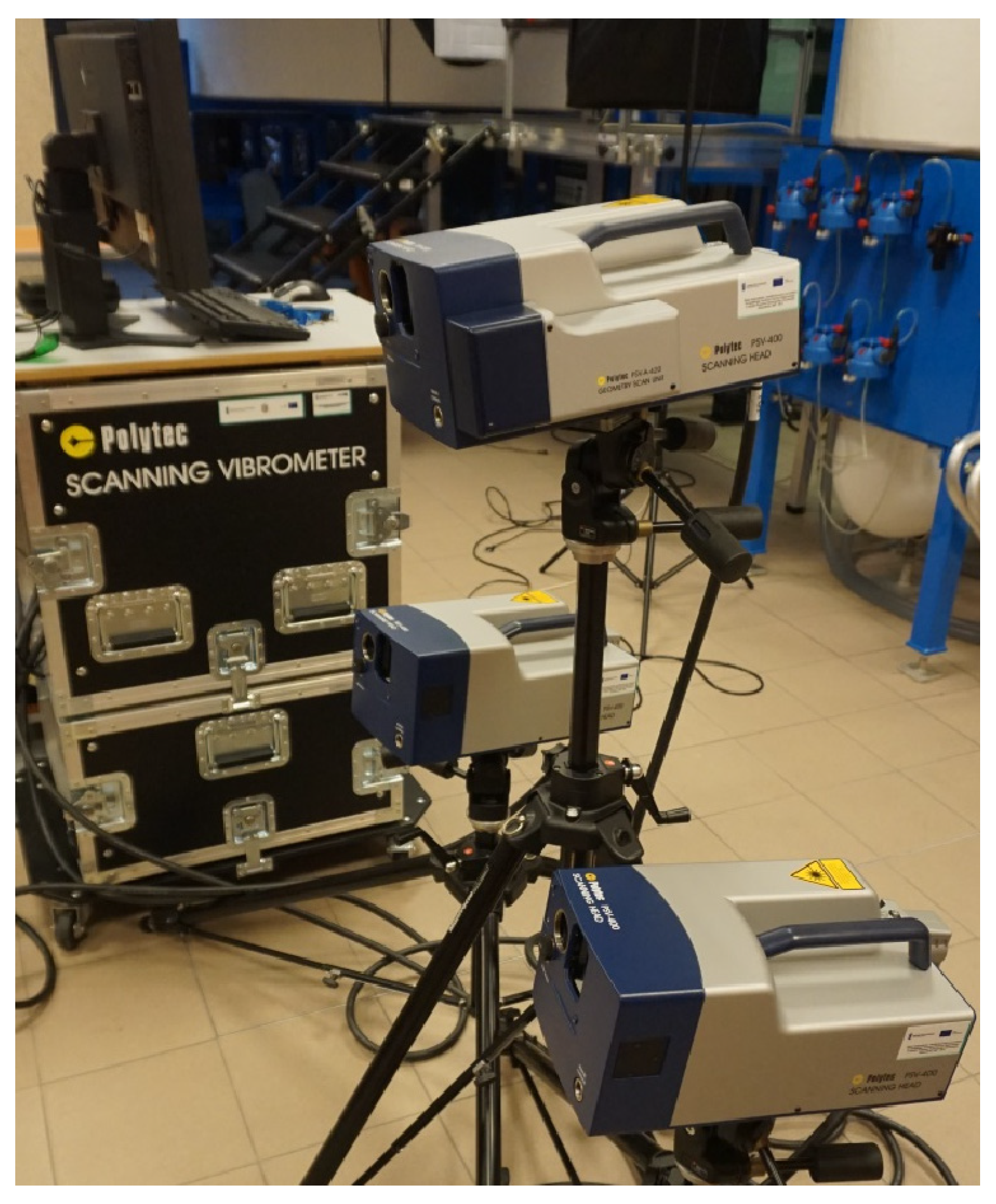
The POLYTEC PSV-400-3D laser vibrometer (Figure 1) is a device that allows for the analysis and visualization of all types of structural vibrations. Its operating principle is based on the splitting of a laser beam generated in the head. One part remains internal and serves as a reference beam, while the other is an emission beam directed at the surface of the tested object. The returning beam is captured by a camera and compared with the reference. Based on this, the instrument determines the displacements on the element and adjusts them to the frequency set by the generator. The 3D measurement involves determining three displacement vectors (three scanning heads) and then, based on these, determining the components in all three directions [5].

Using three independent scanning heads and three controllers, vibration velocity is measured simultaneously in all three directions at the points of a vibrating structure. The three transducers are controlled simultaneously by the PSV central unit and dedicated software. The entire surface of a given object can be automatically scanned according to a pre-defined grid of measurement points. Dedicated software analyses the collected measurement data and, based on it, creates animations depicting the vibration modes of the object across a wide frequency range. An additional geometry scanning module is used to measure and virtually map the object’s measurement surface. The main applications of the laser scanning vibrometer include solving problems related to noise and operational vibration, with particular emphasis on vibration in automotive and aerospace products.

Optical interference can be observed when two coherent light beams converge [6,7]. The resulting intensity, for example, at a photodetector differs from the phase difference Δφ between the two beams according to the equation:

$$I\left(\phi \right)={\displaystyle \frac{I_{max}}{2}}·(1+cos\phi )$$

(1)

The phase difference Δφ is a function of the path difference ΔL between the two beams, according to the formula:

$$\phi ={\displaystyle \frac{L}{\lambda }}·2\pi$$

(2)

where λ is the laser wavelength. If one of the two beams is reflected from a moving object (the object beam), the path difference becomes a function of time ΔL = ΔL(t). The interference fringe pattern moves across the detector, and the object displacement can be determined by directional fringe transition counting. The velocity component in the direction of the object beam is a function of the path difference L depending on:

$${\displaystyle \frac{dL(t)}{dt}}=v(t)·2\pi$$

(3)

For a constant propagation velocity v, the following relationship can be defined:

$$\left|{\displaystyle \frac{dL(t)}{dt}}\right|={\displaystyle \frac{\lambda }{2\pi }}·\left|{\displaystyle \frac{d\phi }{dt}}\right|=f_D·\lambda =\left|v\right|·2$$

(4)

This leads to a frequency shift defined by the expression:

$$f_D={\displaystyle \frac{\left|v\right|}{\lambda }}·2$$

(5)

Thus, the motion of an object causes a frequency shift in the object beam, which is called the Doppler shift f_D and is a function of the velocity component in the direction of the object beam. The master object beam and the internal reference beam, i.e., two electromagnetic waves with slightly different frequencies, generate an excitation frequency in the detector, which is equal to the Doppler shift. Expression (5) is used to determine the velocity and is independent of its sign. The direction of the velocity can be determined by introducing an additional constant frequency shift f_B in the interferometer, to which the Doppler shift with the appropriate sign is added. Thus, the final frequency in the detector f_mod is calculated by the formula:

$$f_{mod}=f_B+{\displaystyle \frac{v}{\lambda }}·2$$

(6)

3. Tested Object

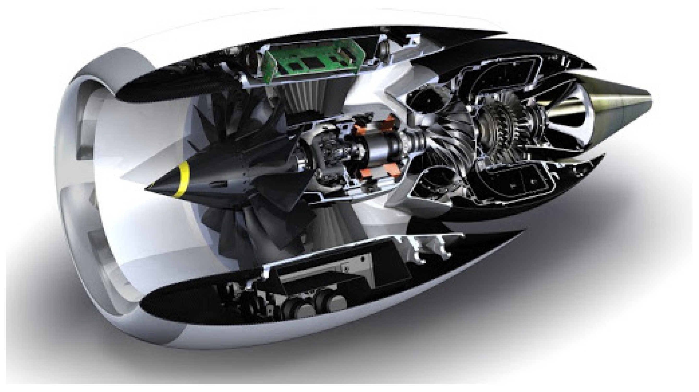
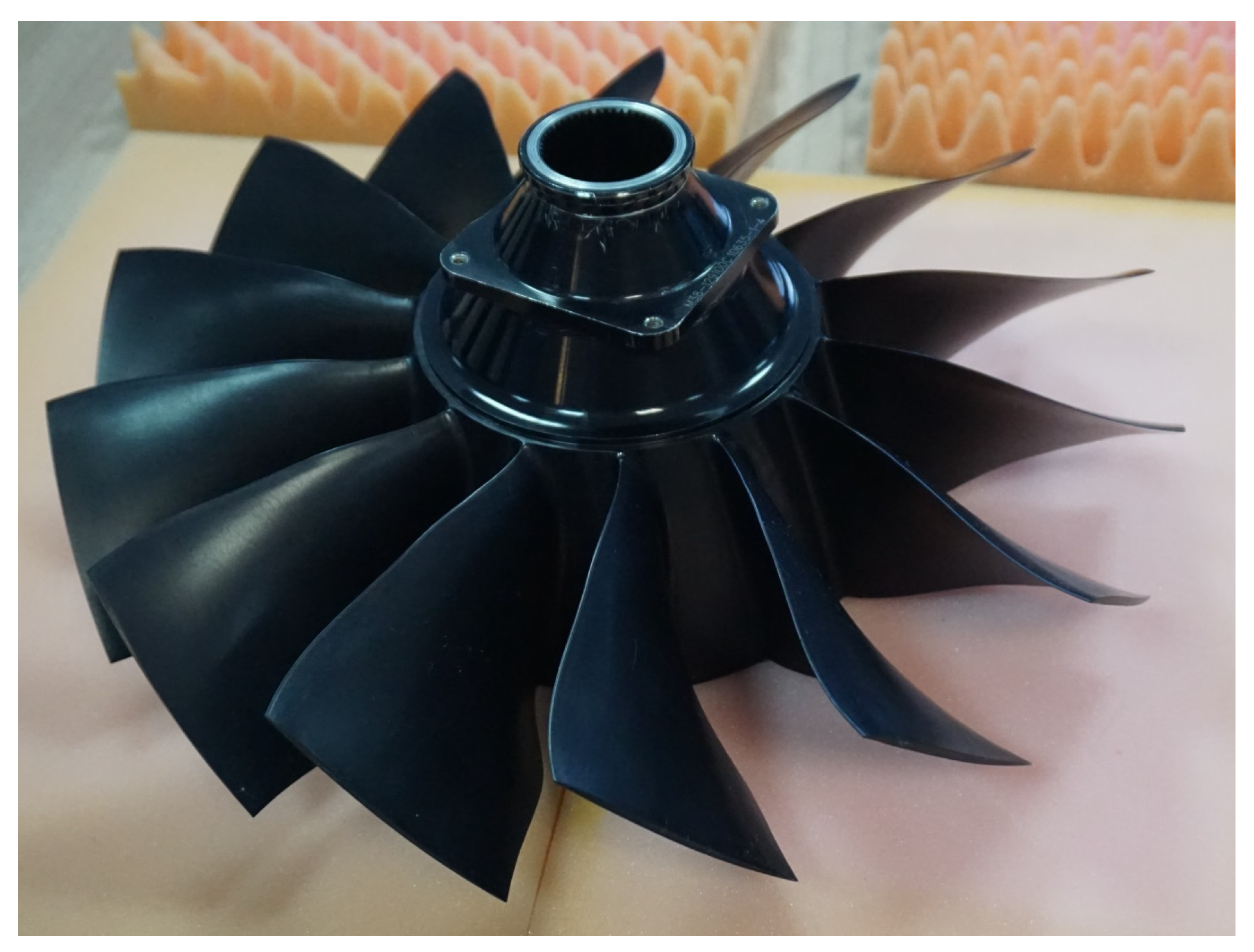
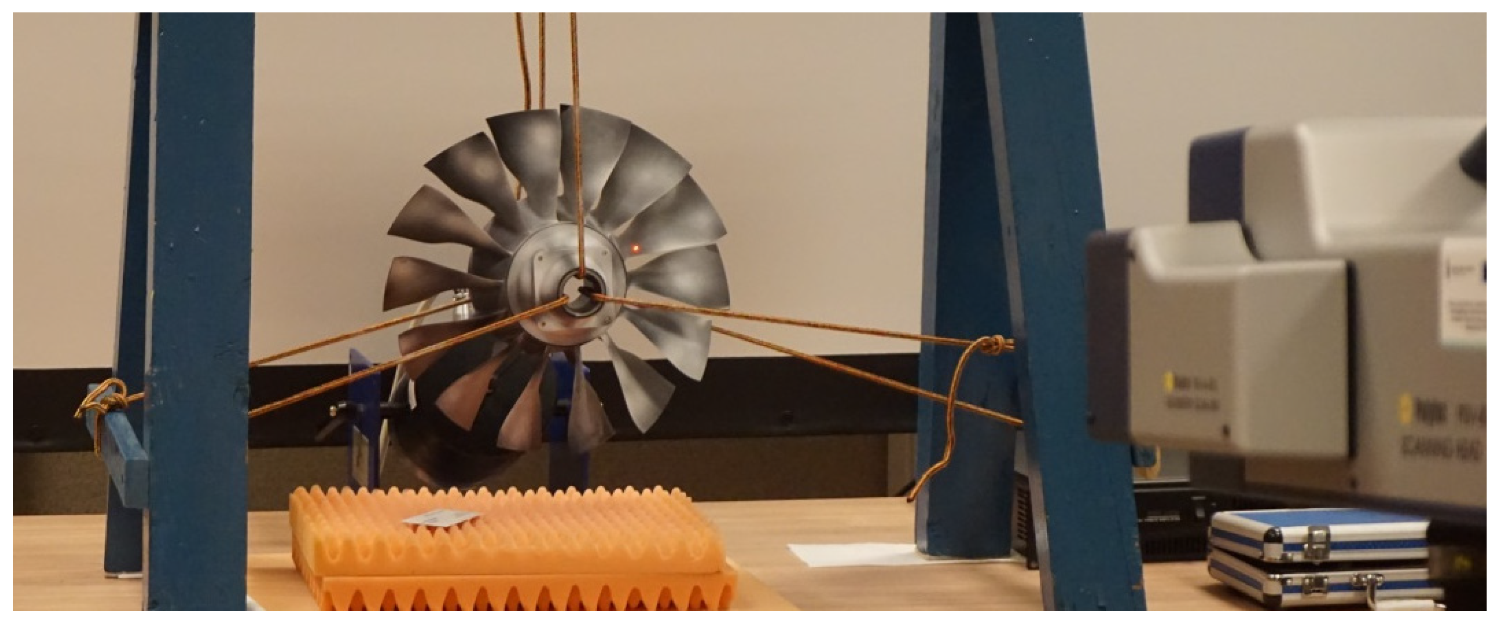
The test element is the isolated first compressor stage of the DGEN-380 miniature jet engine (PRICE INDUCTION, Anglet, France, Figure 2). It is a very complicated object to be examined using the laser method. The disc has the shape of a hollow truncated cone with large blades (Figure 3). For measurements, a disc was suspended inside the frame on flexible wires. In this way, conditions similar to real conditions were ensured. The forcing was carried out by a modal exciter that performs strikes at one point on the back of the shield. Vibration measurements were carried out in a non-contact manner using the Polytec PSV-400-3D scanning Doppler vibrometer.

To replicate the actual setup, the disc was mounted inside a rigid frame using three tensioned rope slings (Figure 4). An electrodynamic exciter from The Modal Shop 2100E11 with a QSC RMX 450 amplifier was used for excitation. The excitation signal was generated by a measurement device (Junction Box). Excitation to the object was achieved by striking it with a stinger with a rubber cap. The excitation point was located on the undercut of the fan’s closing ring, opposite the upper mounting point. The manufacturer’s dedicated PSV 8.7 software was used for acquisition and measurement [9].

4. Results

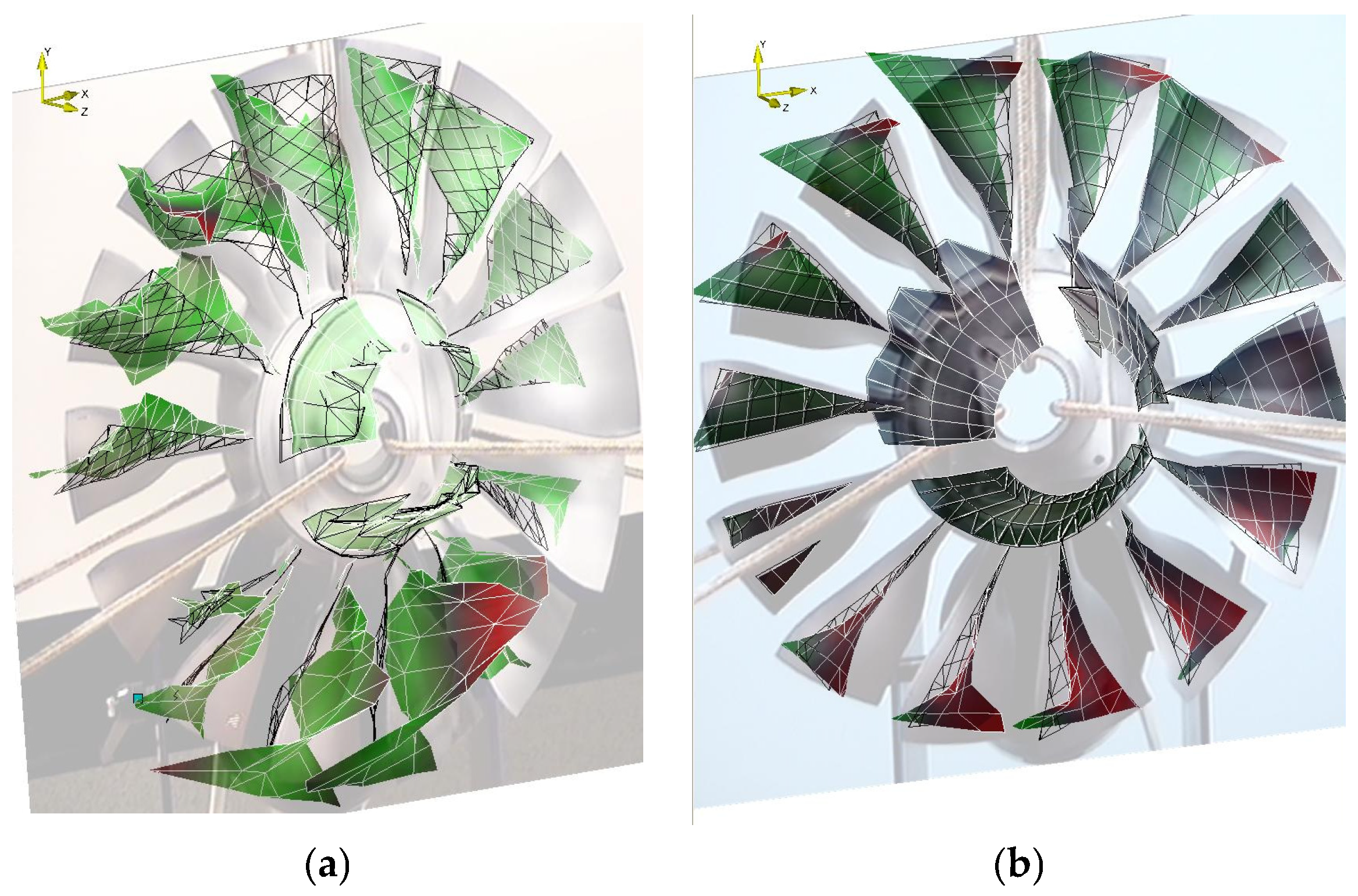
During the experiment, the natural vibration modes of the Dgen-380 engine fan rotor were measured using a laser vibrometer. Two measurement modes were used: 1D, with measurements along the inflow axis, and 3D, with measurements in all three axes. In both modes, the geometry of the object posed a significant challenge, as the laser spot often missed the object at the trailing edges of the blades and at the inflow edge above the connection with the disc. For scan points with the status Overrange, Invalidated or Disabled, the software does not display any measurement data. Researchers can interpolate and display data from neighbouring scan points for these scan points. If they have user-defined data sets available, they can disable, interpolate, and show points individually for each data set. The original data remain unaffected. During interpolation, the distance of a scan point is interpolated from the distances of the neighbours of this point. Then the coordinate is calculated from this distance and the position of the point on the video image. If the point has no neighbours with coordinates, the coordinate remains unmeasured and the dialogue is displayed again. The command Interpolate Data represents measures taken to rid measurements of interference signals and noise levels. When defining the quantity of scan points, it should already be ensured that there is a sufficient scan point density, depending on the shape and expected direction of the maximum amplitudes of the measured object. Careful scan point definition also helps avoiding interference signals caused by unsuitable selection of scan points, e.g., glancing incidence at the edge of an object or undesirable measuring in object openings.

Table 1. Summary of natural frequency results measured with 1D and 3D techniques.

No.	Modes from 1D Measurement [Hz]	Modes from 3D Measurement [Hz]	Δ [Hz]
1	445.3125	446.875	1.5625
2	473.4375	473.4375	0
3	600	600.7813	0.7813
4	900	1063.281	163.281
5	1296.875	1299.219	2.344
6	1515.625	-	-
7	1653.125	1654.688	1.563
8	1778.125	1778.906	0.781
9	1831.25	1839.063	7.813
10	2285.938	2282.813	3.125
11	3114.063	3114.844	0.781
12	3360.938	-	-
13	3426.563	3427.344	0.781
14	3471.875	3474.219	2.344
15	3526.563	3528.906	2.343
16	4020.313	4020.313	0
17	4057.813	-	-
18	4090.625	4080.469	10.156
19	4114.063	4111.719	2.344
20	-	4195.313	-
21	4989.063	4989.844	0.781
22	5564.063	-	-

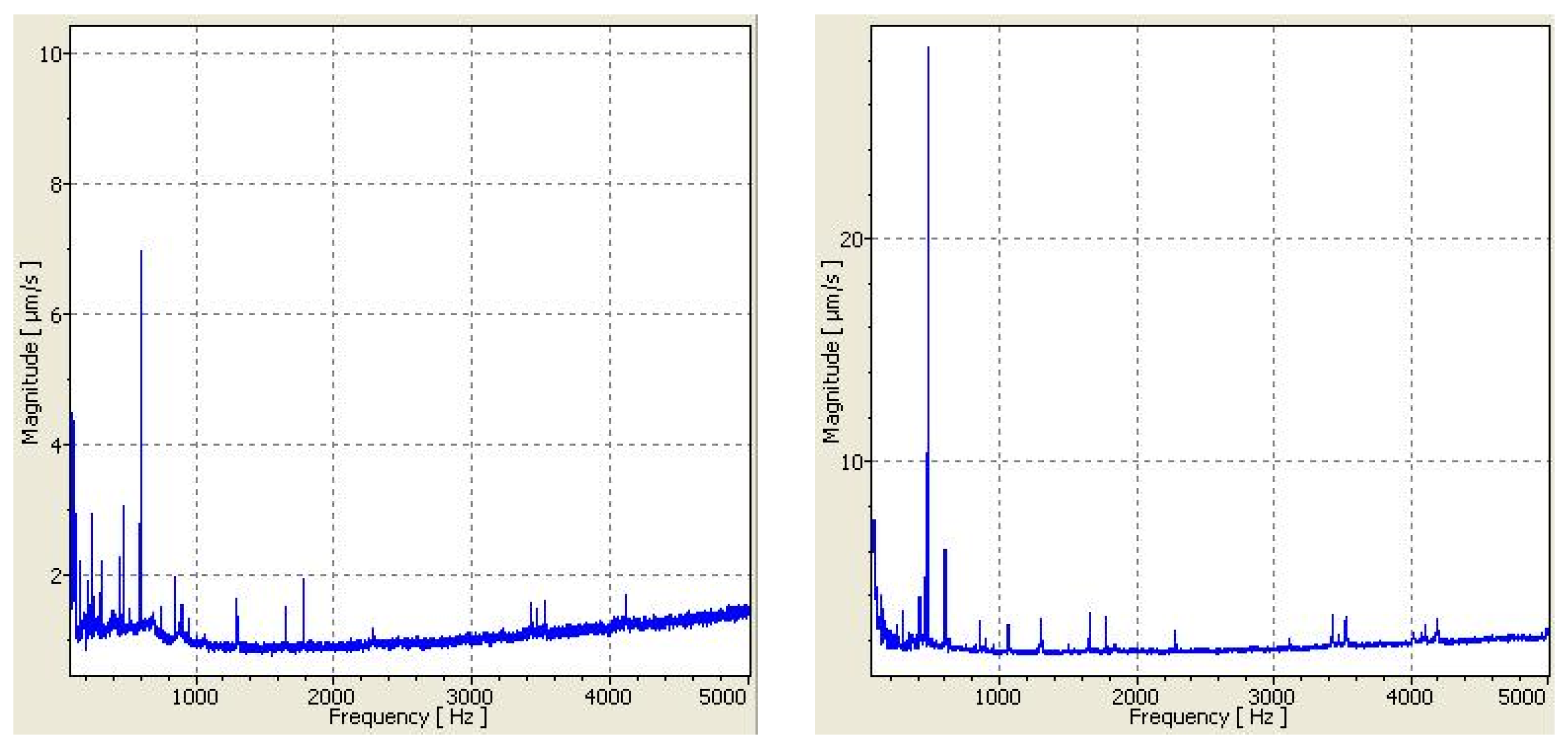
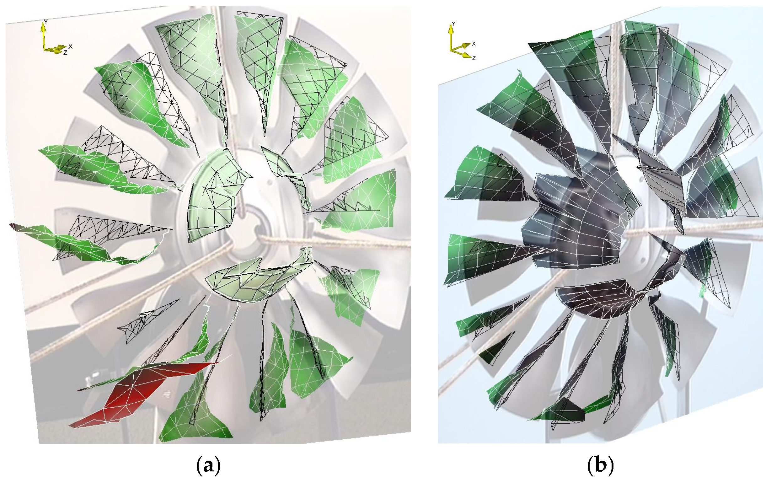
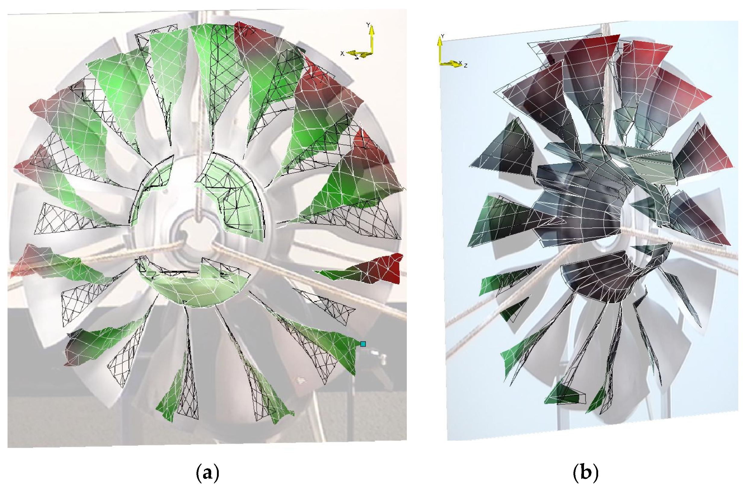
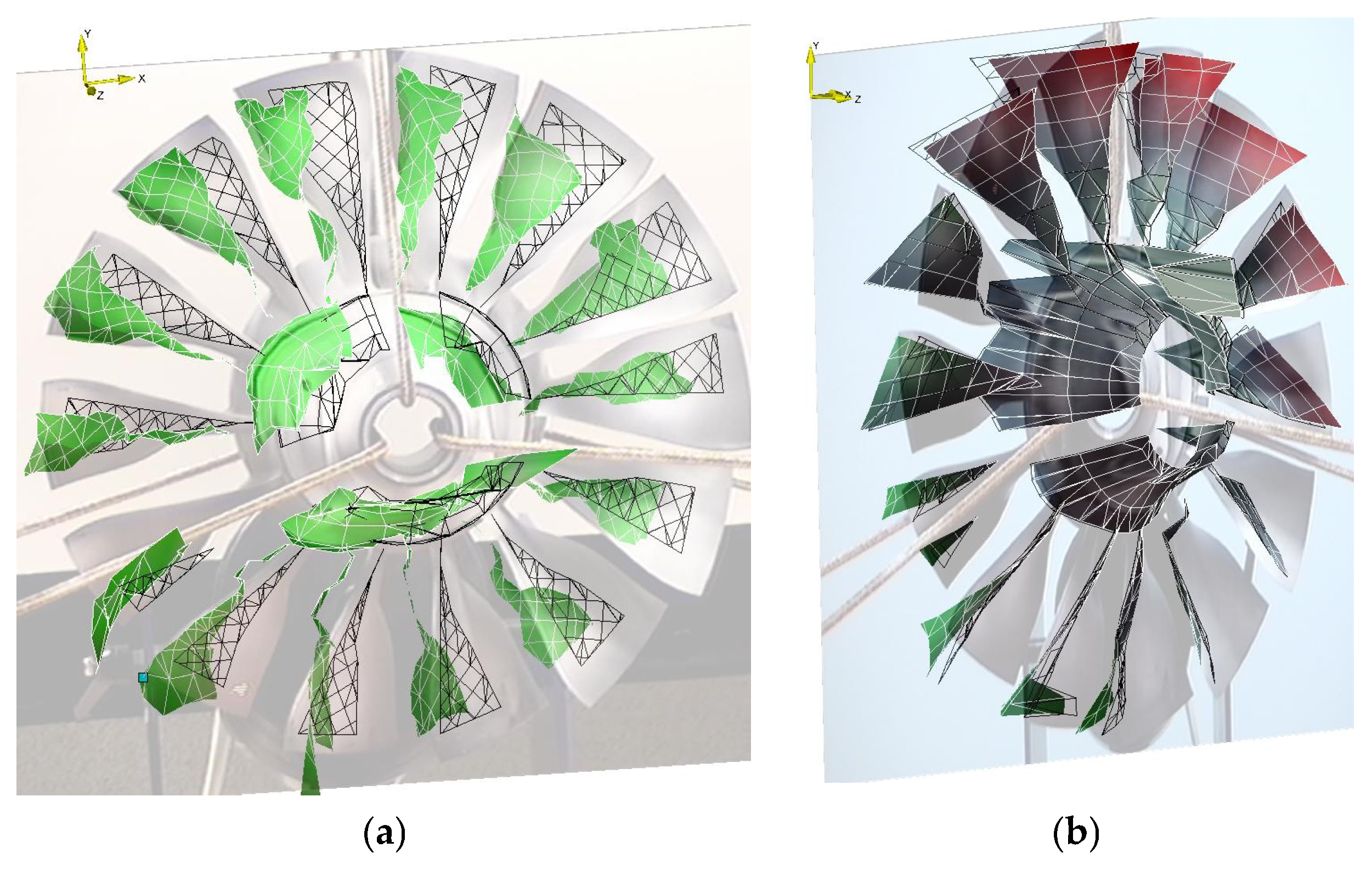
summarizes the obtained frequencies. Figure 5 show average spectrum of measurements. Figure 6, Figure 7, Figure 8 and Figure 9 show four selected pairs of natural vibration modes. Green color indicates movement in the positive direction (towards the head), while red indicates movement away from the head.

5. Conclusions

The measurement was made in 1D and 3D mode. Both measurements were carried out under the same forcing conditions. The 1D mode is simpler and easier to prepare. Only one head is needed. For measurement, the head is set in the axis of rotation of the rotor. The vibrations are represented as unidirectional, parallel to the object-head axis. The 3D mode is more complicated. Three heads must be placed on an equilateral triangle plan with the tested element in the middle. Each head must be calibrated separately and then all must be aligned together. Each head is set at a different angle. This results in three vectors. Determining the mutual position of the heads allows to determine the resultant vector in three-dimensional space. Since the point of the measuring grid must be in the measuring area of each scanning head to measure, it significantly limits the available area. Therefore, the scanned surface is smaller than the area in 1D mode. In 3D mode, the calibration of the three probes greatly complicates measurement preparation. In addition, it is necessary to have advanced and more expensive equipment consisting of three independent heads and three separate controllers. But it allows researchers to get deformation in three-dimensional space.

Figure 4, Figure 5, Figure 6, Figure 7 and Figure 8 show four selected pairs of natural vibration modes. The greatest differences occur in modes with contribution of lateral or angular displacements. This is most visible in mode 4, presented in Figure 7. The disc is being bent simultaneously with the blades. In the 1D mode, this motion resembles spinning around a displaced axis. Furthermore, in the 3D mode, a larger area of the disc’s truncated cone is covered. This is due to the positioning of the heads. In the 1D mode, the axial positioning of the head causes the beam to become tangential to the disc curvature near the blade attachment.

The 1D mode allowed for a better interpretation of the disc vibrations than the 3D mode. Displacements are measured only along the Z axis, which corresponds to the direction of airflow into the engine. There are no displacements in other directions, as in 3D mode, making it easier to interpret the vibration mode or determine the number of nodes. The scanning head is positioned directly in front of the object, ensuring axially symmetrical beam angles and allowing for more precise alignment of the measurement grid to the object’s surface. In 3D mode, three heads are used, which must be properly aligned to ensure that all three laser beams strike the same point with the highest possible accuracy (1.5–0.5 mm). Each beam is positioned at a different angle, so often on curves, one beam misses the object or is obscured. This necessitated reducing the grid size at the edges. As a result, the grid field covered a smaller area than the grid for 1D mode. The blade vibrations can be easily observed from the 3D measurement. For the 1D measurement, the mesh was adequate for analyzing the measured mode sizes, while for the 3D measurement, the mesh was sufficient for analyzing the basic vibration mode sizes, but it should be finer for more accurate interpretation. Because each measurement always involved a dozen or so points being interpolated or measured at the upper tolerance, the amplitude-frequency spectrum is noisy, which complicates interpretation. Interpretation of small amplitudes is highly difficult with noise. Despite this, both methods achieved a number of distinct mode sizes, and the difference between the methods, except for one case, was less than 1%.

References

- Kaliski, S.; Solarz, L.; Dzygadlo, Z.; Wlodarczyk, E. Drgania i Fale w Ciałach Stałych; Państwowe Wydawnictwo Naukowe: Warsaw, Poland, 1966. (In Polish) [Google Scholar]
- Lipka, J. Wytrzymałość Maszyn Wirnikowych; Wydawnictwa Naukowo-Techniczne: Warszawa, Poland, 1967. (In Polish) [Google Scholar]
- Rao, S.S. Mechanical Vibrations, 5th ed.; Pearson Education, Inc.: London, UK, 2011. [Google Scholar]
- Szczeciński, S.; Balicki, W.; Chachurski, R.; Głowacki, P.; Kawalec, K.; Kozakiewicz, A.; Szczeciński, J. Lotnicze Zespoły Napędowe; Wojskowa Akademia Techniczna: Warszawa, Poland, 2009. (In Polish) [Google Scholar]
- Software Manual—Polytec Scanning Vibrometer, Software 8.7; Polytec Deutschland: Waldbronn, Germany, 2009.
- Olejnik, A.; Rogólski, R.; Szcześniak, M. Non-contact Vibration Measurement of Selected Rotor Elements from Aircraft Turbine Engines. Probl. Mechatron.—Armament Aviat. Saf. Eng. 2018, 9, 129–146. (In Polish) [Google Scholar] [CrossRef] [Scilit]
- Theory Manual—Polytec Scanning Vibrometer; Polytec Deutschland: Waldbronn, Germany, 2007.
- Sutliff, D.; Upadhyay, P.; Gold, J. DGEN380 Aero-propulsion Research Turbofan (DART)—Status Update. In Acoustics Technical Working Group Meeting; NASA Glenn Research Center: Cleveland, OH, USA, 2023. [Google Scholar]
- Hardware Manual, Polytec Scanning Vibrometer; PSV-4003D; Polytec GmbH: Waldbronn, Germany, 2011.