Machine Learning-Based Resolution of Strategic Conflicts in U-Space Airspaces ^†

Abstract

The rapid expansion of Unmanned Aircraft System (UAS) operations has created an urgent need for scalable strategic conflict resolution methods within the U-space framework. When requested 4D flight plans overlap with previously authorised ones, the Flight Authorisation Service (FAS) denies the request, and can provide the UAS operator with an alternative route, free of conflict. This work introduces a Machine Learning-based tool designed to support this process, which consists of three sequential phases. First, an Octree spatial partitioning technique is proposed, discretising the airspace, further identifying the previously occupied cells and visualising the occupied airspace, so that the UAS operator can manually find an alternative route. Then, the widely known A* pathfinding algorithm is implemented in this discretized airspace, allowing the shortest or most optimal conflict-free alternative route. Finally, the methodology integrates a Machine Learning (Reinforcement Learning) model, created from scratch and trained with realistic flight trajectories from a PX4 Simulator, to further optimise flight paths, explicitly accounting for operational constraints such as distance and battery consumption. In this work, both methods are compared, addressing traditional algorithms limitations with Machine Learning (ML) techniques, showing that a near-optimal behaviour can be achieved with the ML approach, at a fraction of the computation time needed.

1. Introduction

In recent years, the demand for Unmanned Aircraft Systems (UASs) has increased steadily across multiple domains, creating an urgent need to effectively manage and standardise the emerging U-space airspace to ensure safety and operational efficiency. With this purpose, research works are being carried out all around the globe, especially when it comes to combining two emerging technologies, UASs and AI [1].

Within U-space services, the Flight Authorisation Service (FAS) checks whether a requested 4D flight plan overlaps spatially and temporally with previously authorised traffic. Non-overlapping plans are typically approved, whereas overlapping ones are rejected: conflicts are detected but not resolved. To support strategic conflict resolution, this work proposes a three-stage tool that provides alternative, optimised routes [2]. First, the tool generates a 4D graphical representation of the occupied airspace, enabling operators to visually identify candidate routes. Second, an A* (A-star) pathfinding algorithm is applied in the discretised space to obtain a conflict-free reference trajectory. Third, a Reinforcement Learning (RL) approach is introduced as an alternative to compute near-optimal routes at lower computational cost.

A* is a well-established graph-search algorithm that, under certain conditions, guarantees globally optimal paths, but its computational cost grows exponentially with route length, especially in 3D environments. In contrast, Deep RL (DRL), and in particular a Deep Q-Network (DQN), can scale more favourably while still approximating optimal solutions. In this paper, A* and a DRL-based policy are compared on U-space-like scenarios derived from PX4 simulations [3].

Deep RL has shown the potential to replicate or improve classical algorithms [4] and has been applied to path planning [5] and aerial routing [6]. However, its application to UASs in complex U-space scenarios is still limited.

In this work, A* and a DRL-based policy are compared to assess whether near-optimal paths can be obtained with lower computation times, showing promising results for DRL.

2. Materials and Methods

2.1. Airspace Discretisation and Cell Representation

The airspace is discretised using an Octree structure, dividing the 3D environment into cubic cells and extending them with a temporal dimension. Each flight occupies a sequence of 4D cells (latitude, longitude, altitude and time). When a new request is received, the system identifies all previously occupied cells within the spatial and temporal bounds of the candidate trajectory (the original one plus some extra cells) [7].

2.2. Conflict Detection Workflow

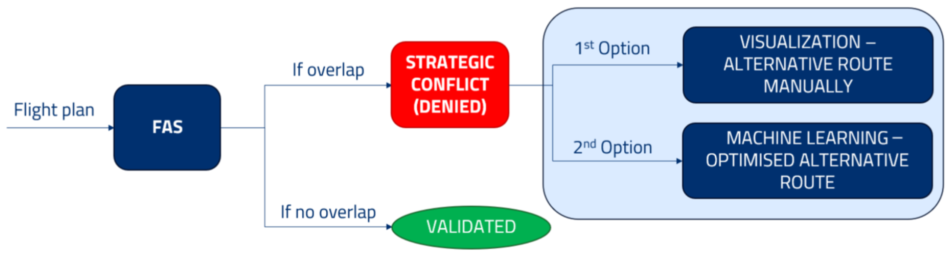
This tool is connected to the FAS, whose database is located in a MySQL server (version 8.0, Oracle Corporation, Austin, TX, USA). If a flight plan is rejected, the tool will detect it and obtain its corresponding Operational Intent (OI)—similar to the flight plan. As shown in Figure 1, if a strategic conflict is detected, the tool offers two different solutions: First, the visualisation of the occupied airspace (as explained previously). Then, the ML-optimised alternative route, which allows for the optimisation of distance and energy.

2.3. Energy Model

An approximate energy model was developed to assign a relative energetic cost to each manoeuvre, combining power and energy-per-distance data from [8,9]. Due to the lack of detailed manoeuvre-based consumption data, the model is a first-order approximation and assumes a multirotor (quadrotor) platform [10].

Several simplifications were applied: wind and aerodynamic interactions were ignored, battery mass was considered constant, and only turning or vertical transitions were assumed to generate acceleration effects. All manoeuvres were assumed feasible, and hover or fixed-wing dynamics were not considered.

The resulting normalised costs (dimensionless, relative to a straight segment) are shown in

Table 1. Final normalised energy costs for all manoeuvres.

Section	Manoeuvre	Cost	Manoeuvre	Cost
Basics	Straight segment	1.0000	Ascent moving 1	1.0012
	Vertical ascent	0.0488	Double ascent moving 2	2.0024
	Vertical descent	0.0323	Descent moving	1.0005
	Double descent moving	2.0010
Diagonal Movements	Straight segment	1.4142	Ascent	1.4151
	Double ascent	2.8302	Descent	1.4146
	Double descent	2.8292
45° turns	Horizontal	1.4616	Descending turn	1.3467
	Double descending	2.6934	Ascending turn	1.3474
	Double ascending	2.6948
90° turns	Horizontal	1.9233	Descending turn	1.6931
	Double descending	3.3862	Ascending turn	1.6939
	Double ascending	3.3878
135° turns	Horizontal	2.8849	Descending turn	2.5396
	Double descending	5.0792	Ascending turn	2.5408
	Double ascending	5.0816
180° turns	Horizontal	4.3273	Descending turn	3.8094
	Double descending	7.6188	Ascending turn	3.8112
	Double ascending	7.6224

¹ Moving: It is being done while moving horizontally as well. ² Double ascent: Case when the drone is going downwards in movement and starts going upwards in movement. It is simplified to ascent twice.

. The low cost of vertical ascent reflects the reduced altitude size of each cell, whereas combined turning–ascending manoeuvres (e.g., double ascending 180° turns) result in the highest relative cost.

2.4. Reference Method: A* Pathfinding

A* is a classical graph-based pathfinding algorithm that extends Dijkstra’s method with a heuristic function, making the search more efficient. In Equation (1), its mathematics are explained [11].

$$f\left(n\right)=g\left(n\right)+h\left(n\right),$$

(1)

where

• $g\left(n\right)$ is the accumulated cost from the initial node to the current node n.
• $h\left(n\right)$ is the heuristic function. It estimates the remaining cost from the current node n to the goal. It should always underestimate the remaining distance; that is why the Euclidean distance is often used here.
• $f\left(n\right)$ is the total cost of the most efficient path from the initial point to the goal while travelling through n.

Under certain conditions that are met in this work, this algorithm ensures the most efficient (absolute optimal) path. By default, it is used for distance optimisation. However, the cost functions can be modified to optimise the desired variables. In this work, both distance and energy are optimised, so the energy costs are included in the cost function.

However, these graph-based classical algorithms, despite being the most precise approach, have an extremely high computational cost, especially when it comes to long routes and 3D environments. Equation (2) shows that the computational complexity (proportional to cost) grows exponentially with the distance of the route [11].

$$O\left(b^d\right),$$

(2)

where

• b is the branching factor (number of adjacent nodes to the current node), which is 26 due to the 3D environment ($3^3-1$).
• d is the route length, which quickly becomes prohibitive for long trajectories.

This is the main flaw of the algorithm, and the objective of this work is to develop an RL model that performs similarly to A* (ideally equal) and finds paths at a fraction of the computational cost.

2.5. Proposed Alternative: RL Model

As an alternative, we use Deep Q-Learning (DQN), which is a form of Reinforcement Learning (RL) that combines Q-learning with deep neural networks (DNNs) to handle large state spaces [12,13].

The computation time of an RL model is given by the computational complexity, shown in Equation (3), where d is the distance of the route, showing that time grows linearly with it.

$$O\left(d\right),$$

(3)

The model used has been created using Python (version 3.10, Python Software Foundation, Wilmington, DE, USA) with the stable-baselines3 (version 2.0, Stable Baselines3 Team, San Francisco, CA, USA) library by OpenAI (San Francisco, CA, USA). These models base their learning on an Agent that learns from a training process, and it basically learns to perform based on a reward function. From the state space it sees, it predicts the expected reward and from the Action Space it chooses the action that is likely to provide the highest reward signal, further maximizing it.

Then, the state space has been designed as follows.

The state space includes the one-hot-encoded current direction (26 elements), the normalised direction to the goal (3), a vision vector indicating whether adjacent cells are obstacles or out of bounds (26), a binary vector marking whether the goal lies in any neighbouring cell (26), and the normalised Euclidean distance to the goal (1).

The reward function is one of the most important parts of the model, since it determines its final behaviour. See Equation (4).

$$R={\alpha }_d·R_d+{\alpha }_e·R_e+{\alpha }_s·R_s+R_t,$$

(4)

where

• $R_d=d_{prev}-d_{next}$ (distance improvement, positive if gets nearer the goal);
• $R_e$ penalises energetically inefficient actions (energy model);
• $R_s$ is a fixed step cost;
• $R_t$ is the terminal reward ($+10$ goal, $-50$ collision/out);
• ${\alpha }_d,{\alpha }_e,{\alpha }_s$ are the corresponding weights, adjusted accurately.

2.6. Training Process

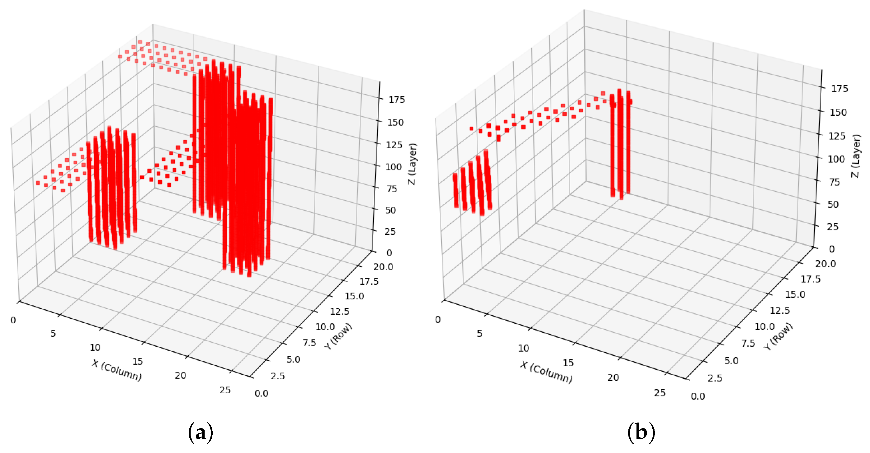
The model has been trained with synthetic data created from realistic flight trajectories generated by the PX4 (version 1.14, Dronecode Foundation, Zurich, Switzerland) SITL Simulator [3]. These have been taken as a reference to synthetically create new trajectories pseudo-randomly, with the same shape and structure. The similarity between the simulator and the pseudo-random trajectories can be seen in Figure 2. The reason why they have been created pseudo-randomly is to ensure the generalisation of the RL model [14]. As can be noted, the pseudo-randomly generated trajectories have the same shape as the other ones but contain a higher obstacle density. This is intentional, since if the model performs well in (b), it will definitely perform well or even better in the real trajectory, (a).

The training process was carried out for $100,000$ episodes, throughout 100 different scenarios, with start and end points generated randomly at the beginning of each episode, again ensuring the generalisation of the model.

3. Results and Discussion

3.1. Training Results

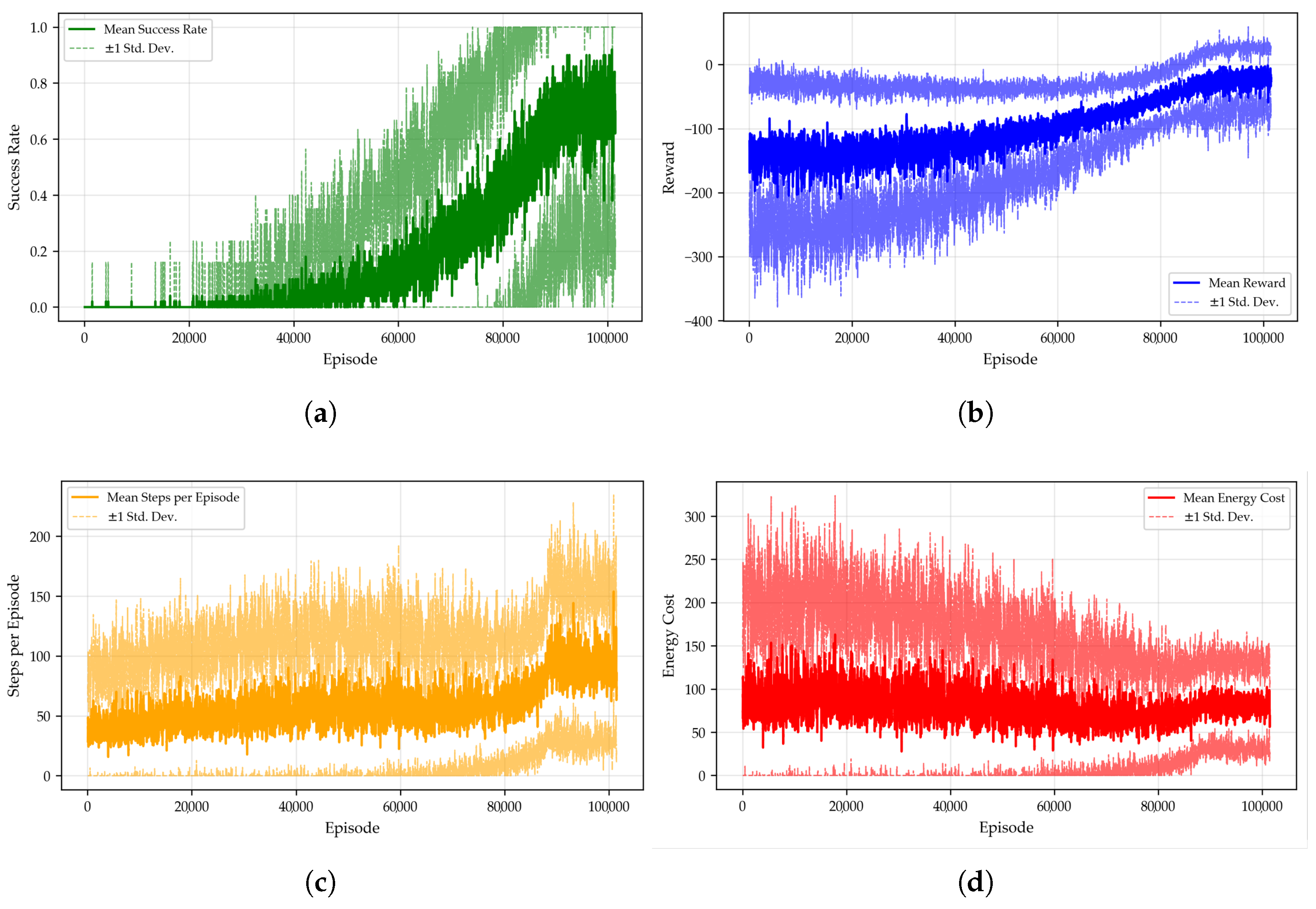
First, the results of the training process are presented in Figure 3.

In Figure 3a, the success rate is shown, improving from 0 at the beginning of the training to $75\%$, meaning that on $75\%$ of occasions, the agent is able to successfully reach the goal without colliding. This shows that the agent learns to achieve the goal, but it does not provide information about how it does it. The episode rewards, portrayed in Figure 3b, show an improvement from $-150$ to around $-20$. The negative sign is not important; what is paramount is that the absolute value of the reward tends to increase throughout the training. This means that the agent has learned to maximise its reward, and consequently, if the reward function has been programmed properly, the agent has learned to successfully optimise distance and energy. Figure 3c shows that the number of steps has increased at the end of the training, which makes sense since routes are longer because the agent collides less often. Furthermore, Figure 3d shows that the energy costs, despite having a high variance, slightly decrease until they stabilise at the end, like the rest of the parameters.

3.2. Evaluation of the Model

Finally, the trained model has been evaluated in different environments generated by the aforementioned PX4 Simulator [3]. Importantly, none of these environments were part of the training dataset, meaning that the agent had no prior exposure to them. This methodology ensures that the results reflect genuine generalisation rather than memorisation, providing a realistic and trustworthy evaluation of the model’s performance.

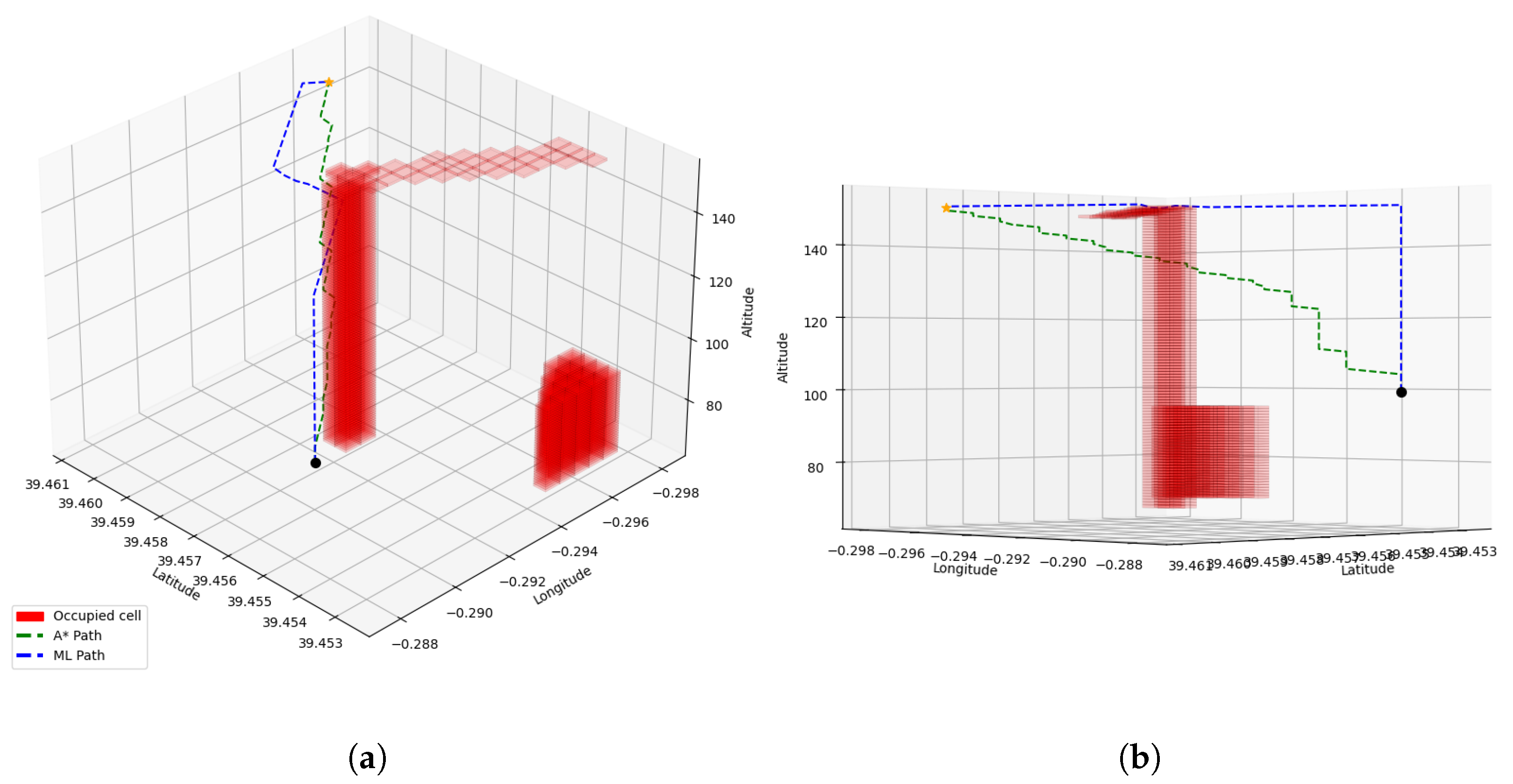
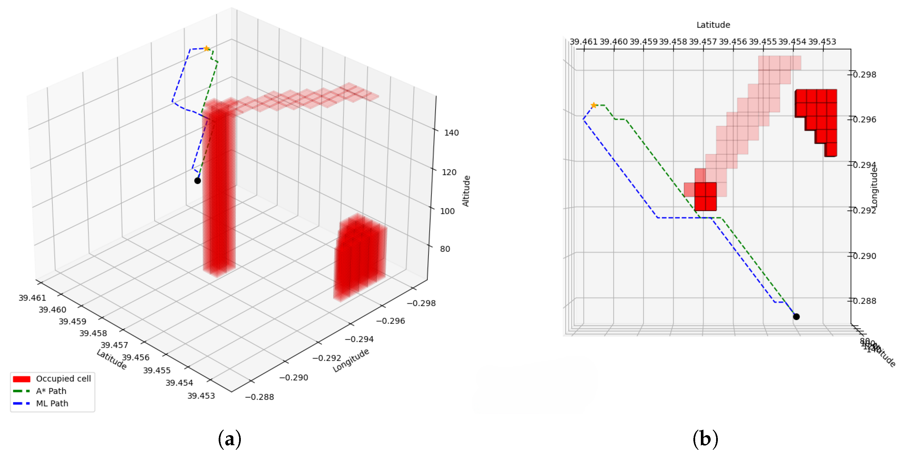
The first scenario evaluation is shown in Figure 4. The blue line shows the A* route while the green line shows the ML one. Both of them get from the start point to the goal while avoiding the red (occupied) cells. Graphically, both are quite similar. In the numerical results, shown in

Table 2. Numerical results of evaluation in the first scenario.

Method	Length [Steps]	Energy [-]	Time [s]
A*	20	26.69	0.023
ML	23	28.43	0.011
Increment [%]	15.00	6.51	−52.00

, it can be noted that the length and the energy increment by $15\%$ and $6.51\%$ while computation time reduces by a half. These results are considered to be near-optimal, since the increment is considered low and noteworthy.

The second scenario is shown in Figure 5. In the horizontal plane, both methods behave similarly, while the main difference appears in the vertical plane due to the altitude change between the start and goal. As seen in

Table 3. Numerical results of evaluation in the second scenario.

Method	Length [Steps]	Energy [-]	Time [s]
A*	66	27.93	35.47
ML	87	31.29	0.038
Increment [%]	32.00	12.01	−99.89

, the DRL route is longer (+32%) and slightly less efficient in energy (+12%), but the key result is the computation time: A* requires $35.47\mathrm{s}$ whereas DRL obtains a solution in only $0.038\mathrm{s}$, a reduction of four orders of magnitude. For longer trajectories, A* scales exponentially (Equation (2)), whereas DRL time increases only mildly (Equation (3)), making the difference decisive in this case.

4. Conclusions

The comparative evaluation of the RL model on previously unseen PX4-derived scenarios shows that the proposed method can achieve near-optimal routes with respect to A* in terms of length and energy, while drastically reducing computation time, especially for longer 3D trajectories where the combinatorial explosion of A* becomes huge, achieving a reduction of four orders of magnitude in simple environments. However, for shorter trajectories, where the time difference is not so notable, A* outperforms ML, being a better option in that case. These results indicate that DRL is a promising candidate for scalable strategic conflict resolution in future large and dense U-space environments. Nevertheless, the current energy model and flight assumptions are intentionally simplified, and the success rate does not yet reach full optimality. Future work will focus on refining the energy model with real flight data, incorporating additional operational constraints (e.g. vehicle-specific limitations), extending the framework to multi-agent conflict resolution and testing the approach in larger, more heterogeneous U-space scenarios.

References

- Obaid, L.; Hamad, K.; Al-Ruzouq, R.; Dabous, S.A.; Ismail, K.; Alotaibi, E. State-of-the-Art Review of Unmanned Aerial Vehicles (UAVs) and Artificial Intelligence (AI) for Traffic and Safety Analyses: Recent Progress, Applications, Challenges, and Opportunities. Transp. Res. Interdiscip. Perspect. 2025, 33, 101591. [Google Scholar] [CrossRef] [Scilit]
- He, S.; Jiang, C. Strategic Conflicts in the Aviation Industry: Evolution and Impact Analysis Using Graph Model with Application to Airspace Conflict between European Countries and Russia. Transp. Econ. Manag. 2025, 3, 199–213. [Google Scholar] [CrossRef] [Scilit]
- Sanchis, A.; Garcia, A.; Esparza, S.; Balbastre, J.V. Realistic Trajectory Generation in Simulated Environments for U-Space Systems Assessment. In Proceedings of the 2025 Integrated Communications, Navigation and Surveillance Conference (ICNS), Brussels, Belgium, 8–10 April 2025; pp. 1–9. [Google Scholar] [CrossRef] [Scilit]
- Mankowitz, D.J.; Michi, A.; Zhernov, A.; Gelmi, M.; Selvi, M.; Paduraru, C.; Leurent, E.; Iqbal, S.; Lespiau, J.B.; Ahern, A.; et al. Faster Sorting Algorithms Discovered Using Deep Reinforcement Learning. Nature 2023, 618, 257–263. [Google Scholar] [CrossRef] [Scilit] [PubMed]
- Lv, L.; Zhang, S.; Ding, D.; Wang, Y. Path Planning via an Improved DQN-Based Learning Policy. IEEE Access 2019, 7, 67319–67330. [Google Scholar] [CrossRef] [Scilit]
- Yao, J.; Li, X.; Zhang, Y.; Ji, J.; Wang, Y.; Zhang, D.; Liu, Y. Three-Dimensional Path Planning for Unmanned Helicopter Using Memory-Enhanced Dueling Deep Q Network. Aerospace 2022, 9, 417. [Google Scholar] [CrossRef] [Scilit]
- Amarillo, S.; Sanchis, A.; Freire, B.F.; Balbastre, J.V. Proposal of UAS Strategic Conflict Detection Concept with a Centralised Service in Multi-USSP Environment Using an Octree Data Structure. In Proceedings of the 2025 Integrated Communications, Navigation and Surveillance Conference (ICNS), Brussels, Belgium, 8–10 April 2025; pp. 1–8. [Google Scholar] [CrossRef] [Scilit]
- Gong, H.; Huang, B.; Jia, B.; Dai, H. Modelling Power Consumptions for Multi-rotor UAVs. arXiv 2022, arXiv:2209.04128. [Google Scholar] [CrossRef] [Scilit]
- Jacewicz, M.; Żugaj, M.; Głębocki, R.; Bibik, P. Quadrotor Model for Energy Consumption Analysis. Energies 2022, 15, 7136. [Google Scholar] [CrossRef] [Scilit]
- Höhrová, P.; Soviar, J.; Sroka, W. Market Analysis of Drones for Civil Use. LOGI Sci. J. Transp. Logist. 2023, 14, 55–65. [Google Scholar] [CrossRef] [Scilit]
- Russell, S.J.; Norvig, P. Artificial Intelligence: A Modern Approach, 4th ed.; global edition; Prentice Hall Series in Artificial Intelligence, Pearson: Boston, MA, USA, 2022. [Google Scholar]
- Sutton, R.S.; Barto, A.G. Reinforcement Learning: An Introduction; The MIT Press: Cambridge, MA, USA, 2014. [Google Scholar]
- Liang, S.; Srikant, R. Why Deep Neural Networks for Function Approximation? arXiv 2017, arXiv:1610.04161. [Google Scholar] [CrossRef] [Scilit]
- Goodfellow, I.; Bengio, Y.; Courville, A. Deep Learning; MIT Press: Cambridge, MA, USA, 2016. [Google Scholar]