Comparative Study of Rigid and Flexible Multibody Dynamics in a 3D-Printed Two-Link Robotic Mechanism ^†

Abstract

The use of 3D printing in robotics enables lightweight, customized, and geometrically complex structures, but the resulting structural compliance challenges accurate dynamic prediction. Traditional rigid multibody models often neglect structural deformations and vibrations that can critically affect performance and control. This work presents initial advances toward a computational framework for flexible multibody dynamics of 3D-printed robotic structures. A two-link mechanism is modeled in MATLAB Simscape Multibody under both rigid and flexible assumptions, and parametric analyses are conducted to assess the influence of geometry, mass distribution, and stiffness on system dynamics. The proposed framework is formulated to accommodate reduced-order and data-driven modeling approaches for efficient simulation and analysis of flexible robotic mechanisms.

1. Introduction

The advent of additive manufacturing (AM) is revolutionizing mechanical and robotic systems design by permitting complex geometries that were previously almost impossible using standard subtractive or formative approaches [1,2]. Within this context, the production of lightweight, topologically optimized and functionally graded parts has created a new class of robotic structures that merges mechanical compliance, material efficiency and structural adaptability [3,4]. Among these, metal additive manufacturing has gained eminence for its precision, mechanical integrity, and ability to produce small-scale lightweight components with complex internal features [5,6].

For robotic systems, such design freedom permits engineers to design links and joints that contain integrated compliant mechanisms, built-in flexible elements and have distributed mass properties which improve dexterity and lower energy intake. However, these benefits come with inherent challenges. 3D-printed metallic parts, being light and slim, are more susceptible to elastic deformations, mode coupling, and vibrational instabilities, for instance, when under dynamic loading [7,8]. Common rigid multibody dynamic models assume perfectly rigid links and ideal joints, which usually fail to capture these phenomena, leading to inconsistencies between anticipated and actual system responses during precision tasks.

Rigid multibody modeling still forms the basis for both the kinematic and dynamic analysis of robotic systems, certainly because of its computational and implementation simplicity [9]. Such a modeling approach treats links as rigid mass elements connected via ideal joints and derives the equations of motion by Newton–Euler or Lagrangian formulations. While this assumption has worked well for classical industrial manipulators, made of high-stiffness materials, it becomes less adequate for lighter mechanisms, particularly those that are additively manufactured. In such cases, local flexibility and distributed compliance remain highly critical in the overall system [10,11]. For instance, elastic vibrations can generate oscillations, positional errors, and phase shifts within thin-walled or lattice-reinforced 3D-printed arms. These effects can compromise control accuracy and stability [12].

The insufficiencies of existing methodologies demand the development of a sophisticated modeling scheme capable of capturing both rigid multibody motion and elastic deformation. Flexible multibody dynamics (FMBD) has emerged as an advanced modeling framework capable of capturing both the phenomena within a unified formulation. FMBD allows each link to deform under load, with simultaneous global motion inputs restrained by multibody constraints. The dynamic systems are generally described using finite-element discretization, modal reduction or lumped parameter representations. This method allows us to accurately simulate structural flexibility, vibration propagation, and dynamic coupling between components, particularly relevant for 3D-printed systems.

Several studies have demonstrated that rigid multibody formulations may underestimate vibration amplitudes and phase lag in lightweight robotic manipulators, particularly when link slenderness increases or excitation frequencies approach structural resonances [13,14]. Modal-based flexible multibody formulations, frequently implemented using the floating frame of reference approach, enable the incorporation of structural compliance while maintaining computational efficiency [15]. These formulations express elastic deformation through a truncated modal expansion, allowing dominant bending modes to be captured without full finite-element discretization.

In recent years, simulation environments such as MATLAB R2025a Simscape Multibody have enabled the practical integration of rigid and flexible bodies within a unified modeling framework, facilitating comparative studies and parametric analyses of multibody systems [16]. However, systematic investigations that directly compare rigid and flexible multibody formulations for 3D-printed robotic mechanisms remain limited, particularly with respect to the influence of geometric properties, mass distribution, and structural stiffness.

This study intends to take the first step toward fulfilling this research gap by a comparative analysis of rigid and flexible multibody dynamics for a 3D-printed, two-link metal robotic system, modeled in MATLAB Simscape Multibody. By performing parametric analyses involving variations in geometry, material stiffness, and excitation torque, the study reveals the performance trade-offs between dynamic stability and lightweight design. Beyond conventional finite-element and multibody approaches, the framework is conceived as a foundation for future integration of reduced-order and AI-driven surrogate models, offering real-time predictive simulation necessary for model-based control and design optimization.

2. Materials and Methods

2.1. Design of the Two-Link Robotic Mechanism

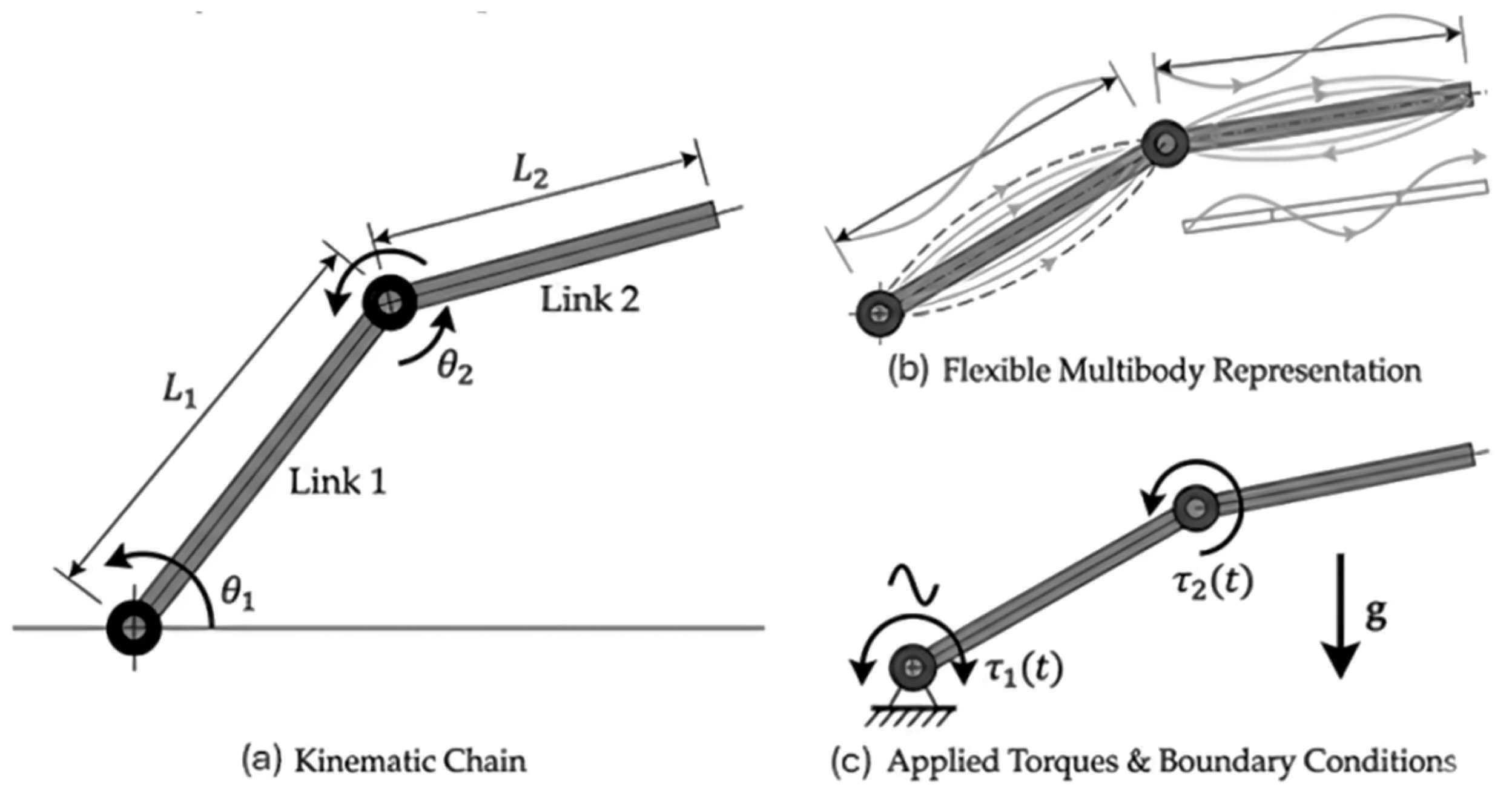
As a case study, a planar two-link robotic mechanism was designed to assess different dynamics using rigid and flexible modeling assumptions, as shown in Figure 1. Each link was to be treated as a uniform prismatic beam connected through revolute joints, allowing it to mimic a generic lightweight manipulator structure. The first link is anchored at the base and rotates about the z-axis. The second link is attached to the distal end of the first through a revolute joint. The geometric parameters correspond to a representative lightweight robotic link configuration commonly used in laboratory-scale manipulators and precision positioning systems. The first link has a length of $L_1=0.25\hspace{0.17em}\mathrm{m}$, while the second link has a length of $L_2=0.20\hspace{0.17em}\mathrm{m}$. Mass values m = ρAL were computed from cross-sectional area A and density ρ, ensuring consistency between material properties and inertial parameters. Both links share a rectangular cross-section of $15\times 10\hspace{0.17em}{\mathrm{mm}}^2$.

2.2. Material Properties and Assumptions

The robotic links were modeled using linear elastic material properties representative of Ti6Al4V alloy, which is widely used in lightweight structural applications [17]. The material is assumed to be homogeneous and isotropic, with the properties listed in

Table 1. Material and geometric properties used in the simulations.

Property	Symbol	Value	Unit
Density	$\rho$	4430	kg/m3
Elastic modulus	$E$	110	GPa
Poisson’s ratio	$\nu$	0.33	—
Yield strength	${\sigma }_y$	830	MPa
Link 1 length	$L_1$	0.25	m
Link 2 length	$L_2$	0.20	m
Link 1 mass	m1	0.166	kg
Link 2 mass	m2	0.133	kg
Cross-section	$A=b\times h$	1.5 × 10−4	m2
Damping coefficient	$c$	0.02	N·m·s/rad

[18,19].

The flexible formulation assumes small deformations and linear elastic behavior. No material anisotropies, residual stresses, plasticity, or process-induced effects are included in the present model. While Ti6Al4V is commonly associated with additive manufacturing applications, the present analysis does not model manufacturing process physics. The selected material properties serve as representative values for a lightweight metallic structure.

2.3. Modeling and Mathematical Formulation

In the rigid multibody representation, the configuration of the system is fully described by a vector of generalized joint coordinates,

$${\mathit{q}}_r\left(t\right)={\left[\begin{array}{cc}{\theta }_1\left(t\right)& {\theta }_2\left(t\right)\end{array}\right]}^{\mathsf{T}}$$

(1)

where ${\theta }_1\left(t\right)$ and ${\theta }_2\left(t\right)$ denote the rotation angles of the first and second revolute joints, respectively. The equations of motion are obtained using classical multibody dynamics formulations and can be written as

$$\begin{array}{cccc}& {\mathit{M}}_r\left({\mathit{q}}_r\left(t\right)\right)\hspace{0.17em}{\ddot{\mathit{q}}}_r\left(t\right)+{\mathit{C}}_r\left({\mathit{q}}_r\left(t\right),{\dot{\mathit{q}}}_r\left(t\right)\right)\hspace{0.17em}{\dot{\mathit{q}}}_r\left(t\right)={\mathit{f}}_r\left(t\right),& & \end{array}$$

(2)

where ${\mathit{M}}_r\left({\mathit{q}}_r\right(t\left)\right)$ is the configuration-dependent mass matrix, ${\mathit{C}}_r\left({\mathit{q}}_r\right(t),{\dot{\mathit{q}}}_r(t\left)\right)$ collects Coriolis and centrifugal effects, and ${\mathit{f}}_r\left(t\right)$ is the vector of generalized external forces, including actuation torques and gravity contributions. No stiffness matrix appears in Equation (2), as rigid multibody models do not admit elastic deformation and therefore do not possess intrinsic vibration modes. Any oscillatory response arises from external excitation or nonlinear kinematic coupling.

To account for structural flexibility, each link is modeled as a flexible body undergoing small elastic deformation superimposed on large rigid multibody motion. The generalized coordinate vector of the flexible system is partitioned as

$${\mathit{q}}_f\left(t\right)=\left[\begin{array}{c}{\mathit{q}}_r\left(t\right)\\ \eta \left(t\right)\end{array}\right],$$

(3)

where $\mathit{\eta }\left(t\right)$ denotes the vector of elastic (modal) coordinates. The elastic displacement field of each link is approximated using a modal superposition approach:

$$\begin{array}{cccc}& u(x,t)=\sum _{i=1}^n{\varphi }_i\left(x\right)\hspace{0.17em}{\eta }_i\left(t\right),& & \end{array}$$

(4)

where ${\varphi }_i\left(x\right)$ representing assumed mode shapes, ${\eta }_i\left(t\right),$ the corresponding modal amplitudes, and $x$ denotes the scalar spatial coordinate measured along the undeformed neutral axis of the flexible link. In this study, the reduced-order flexible model retains one bending mode for each link, resulting in two elastic coordinates in addition to the rigid-body generalized coordinates. The equations of motion of the flexible multibody system can then be written in block-matrix form as

$$\begin{array}{cccc}& \left[\begin{array}{cc}{\mathit{M}}_{rr}& {\mathit{M}}_{r\eta }\\ {\mathit{M}}_{\eta r}& {\mathit{M}}_{\eta \eta }\end{array}\right]\left[\begin{array}{c}{\ddot{\mathit{q}}}_r\left(t\right)\\ \ddot{\mathit{\eta }}\left(t\right)\end{array}\right]+\left[\begin{array}{cc}{\mathit{C}}_{rr}& {\mathit{C}}_{r\eta }\\ {\mathit{C}}_{\eta r}& {\mathit{C}}_{\eta \eta }\end{array}\right]\left[\begin{array}{c}{\dot{\mathit{q}}}_r\left(t\right)\\ \dot{\mathit{\eta }}\left(t\right)\end{array}\right]+\left[\begin{array}{cc}0& 0\\ 0& {\mathit{K}}_{\eta \eta }\end{array}\right]\left[\begin{array}{c}{\mathit{q}}_r\left(t\right)\\ \mathit{\eta }\left(t\right)\end{array}\right]=\left[\begin{array}{c}{\mathit{f}}_r\left(t\right)\\ {\mathit{f}}_{\eta }\left(t\right)\end{array}\right].& & \end{array}$$

(5)

In this formulation, ${\mathit{M}}_{ij}$ are mass submatrices that depend/ on the instantaneous configuration of the mechanism, reflecting the time-varying inertia induced by large rigid multibody motion. The matrices ${\mathit{C}}_{ij}$ collect velocity-dependent inertial and damping effects. The stiffness matrix ${\mathit{K}}_{\mathit{\eta }\mathit{\eta }}$ acts only on the elastic modal coordinates $\eta$, while rigid-body coordinates are unaffected by structural stiffness terms. The vectors ${\mathit{f}}_r\left(t\right)$ and ${\mathit{f}}_{\eta }\left(t\right)$ denote generalized forces associated with rigid-body motion and elastic deformation, respectively.

The rigid multibody model is recovered from Equation (5) by neglecting elastic coordinates, i.e., by setting $\mathit{\eta }\left(t\right)=0$, which eliminates stiffness effects and reduces the formulation to Equation (2). This clear separation allows a direct and physically consistent comparison between rigid and flexible representations.

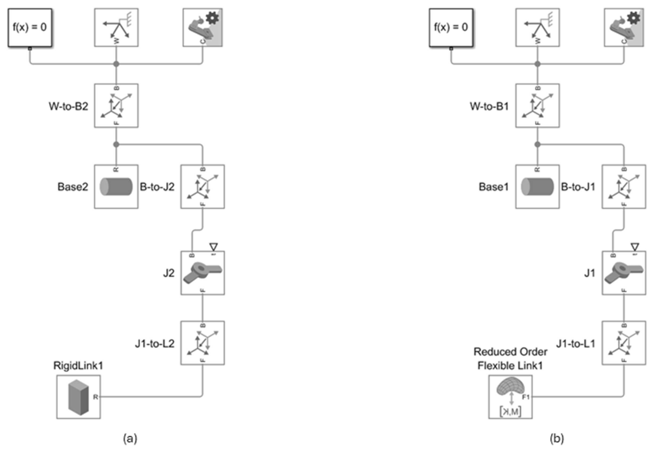
Both models are implemented in MATLAB Simscape Multibody. Rigid bodies are represented as undeformable solids with prescribed mass and inertia properties, while flexible links are modeled using modal-based flexible body formulation in Simscape Multibody, where elastic deformation is represented by a finite number of bending modes appended to the rigid-body motion. In the present study, the generalized coordinates correspond to the two joint angles and the retained bending modal coordinates of each link. The formulation is therefore directly applied to the mechanism shown in Figure 1. Figure 2 presents a Simscape Multibody block diagram representation of a single-link system.

2.4. Simulation Configuration and Boundary Conditions

The system is excited by externally applied actuation torques at the revolute joints. The generalized force vector associated with the rigid-body coordinates is defined as

$${\mathit{f}}_r\left(t\right)=\left[\begin{array}{c}{\tau }_1\left(t\right)\\ {\tau }_2\left(t\right)\end{array}\right]$$

where ${\tau }_1\left(t\right)$ and ${\tau }_2\left(t\right)$ denote the torques applied at the first and second joints, respectively. Each torque is prescribed as a harmonic excitation of the form:

$$\begin{array}{cccc}& {\mathit{\tau }}_i\left(t\right)={\tau }_{i,0}\hspace{0.17em}\mathit{sin}\left(\omega t\right) i=\mathrm{1,2}& & \end{array}$$

(6)

where ${\mathit{\tau }}_{i,0}$ represents the torque amplitude with ${\tau }_{\mathrm{1,0}}=0.25\hspace{0.17em}\mathrm{Nm}$, ${\tau }_{\mathrm{2,0}}=0.15\hspace{0.17em}\mathrm{Nm}$ and $\omega =12\hspace{0.17em}\mathrm{rad}/\mathrm{s}$ is the excitation angular frequency. To enable evaluation of decay and settling behavior, the excitation is applied only during an initial time interval. The torque profile is therefore defined as

$${\tau }_i(t)=\{\begin{array}{cc}{\tau }_{i,0}sin\left(\omega t\right),& 0\le t\le t_{off}\\ 0,& t>t_{off}\end{array}$$

(7)

where $t_{off}$ denotes the excitation termination time. After $t_{off}$, the system evolves under free vibration, allowing the decay characteristics and settling time to be evaluated. Regarding the boundary conditions, joint 1 is fixed at the base frame, joint 2 has free rotation constrained to planar motion; gravity $g=9.81\hspace{0.17em}{\mathrm{m}/\mathrm{s}}^2$.

2.5. Numerical Implementation and Solver Settings

The coupled rigid and flexible multibody models were simulated in MATLAB/Simscape using the variable-step stiff solver ode15s, which is suitable for systems containing high-frequency flexible dynamics and potential numerical stiffness. Relative and absolute tolerances were set to ${10}^{-6}$ and ${10}^{-8}$ respectively. These values were selected to ensure numerical stability while accurately capturing high-frequency modal responses. The Simscape local solver was disabled, and integration was handled by the global solver.

To verify numerical robustness, simulations were repeated with stricter tolerances (${10}^{-7}$ relative tolerance), and variations in key metrics (natural frequencies, RMS displacement, and settling time) were found to be negligible (<1%), confirming numerical convergence.

For frequency-domain analysis, the end-effector displacement signal was analyzed over a fixed steady-state window during the forced excitation phase. The harmonic torque excitation was applied over the interval $0\le t\le t_{off}$, with $t_{off}=3\hspace{0.17em}\mathrm{s}$ and a total simulation time of $5\hspace{0.17em}\mathrm{s}$. A Hanning window was applied prior to transformation to reduce spectral leakage. The frequency resolution was determined as

$$\Delta f={\displaystyle \frac{1}{T_{\mathrm{window}}}}$$

where $T_{window}=t_2-t_1=1\hspace{0.17em}\mathrm{s}$ denotes the duration of the analyzed signal segment.

2.6. Performance Evaluation Metrics

To compare the two models quantitatively, the following evaluation metrics were established. All quantities are evaluated in the planar workspace of the mechanism, and vector norms are computed using the Euclidean (ℓ₂) norm. Some metrics, such as joint angular displacement and settling time, are defined for both the rigid and flexible models. Other quantities, such as elastic vibration amplitude and flexible-mode frequency content, arise only in the flexible formulation due to the presence of elastic coordinates.

• End-effector trajectory deviation: The instantaneous deviation between the flexible and rigid model predictions is defined as

$$\Delta x\left(t\right)=\parallel {\mathit{x}}_f\left(t\right)-{\mathit{x}}_r\left(t\right){\parallel }_2$$

(8)

where ${\mathit{x}}_f\left(t\right)\in {\mathbb{R}}^2$ is the planar end-effector position from the flexible model, ${\mathit{x}}_r\left(t\right)\in {\mathbb{R}}^2$ is the corresponding position from the rigid model, and $\parallel \cdot {\parallel }_2$ denotes the Euclidean norm.

2.

Root-Mean-Square (RMS) vibration amplitude of the tip displacement: The elastic displacement of the end-effector relative to its rigid-body position is defined as

$$\mathit{u}\left(t\right)={\mathit{x}}_f\left(t\right)-{\mathit{x}}_r\left(t\right).$$

The RMS vibration amplitude is computed over a fixed steady-state window during the forced excitation phase $T=[t_1,t_2]$, where $t_1=2\hspace{0.17em}\mathrm{s}$ and $t_2=3\hspace{0.17em}\mathrm{s}$. This interval corresponds to the final 1 s of the forced-response regime, ensuring that initial transients have decayed while the harmonic excitation is still active.

$$u_{\mathrm{RMS}}=\sqrt{{\displaystyle \frac{1}{t_2-t_1}}{\int }_{t_1}^{t_2}\parallel \mathit{u}\left(t\right){\parallel }_2^2\hspace{0.17em}dt}$$

(9)

where $\parallel \cdot {\parallel }_2$ denotes the Euclidean norm. The same evaluation window is used for both the rigid and flexible models to ensure consistency of the comparison.

3.

Settling time of the end-effector oscillation post excitation: Following the termination of harmonic excitation at t = t_off, the system response transitions from forced vibration to a free-decay regime. The settling time is evaluated based on the decay of the oscillatory envelope of the end-effector displacement response. The reference amplitude u_ss is defined as the peak displacement amplitude observed immediately prior to excitation termination within the interval [t₁, t₂], which represents the steady forced-response regime. The settling time is then defined as

$$t_s=min\left\{t\ge 0\hspace{0.25em} |\hspace{0.25em} \mid u_{\mathrm{env}}(\tau )-u_{\mathrm{ss}}\mid \le \epsilon u_{\mathrm{ss}}\forall \tau \ge t\right\}$$

(10)

where $u_{\mathrm{env}}\left(t\right)$ represents the amplitude envelope of the oscillatory response, $\epsilon =0.05$ corresponds to a ±5% tolerance band.

2.7. Damping Model Formulation

Damping was introduced at two levels in the multibody formulation. First, viscous damping was applied at each revolute joint using a linear rotational damping model

$${\tau }_d=c\hspace{0.17em}\dot{\theta },$$

(11)

where c is the joint viscous damping coefficient and $\dot{\theta }$ is the joint angular velocity. This damping accounts for energy dissipation due to joint friction and actuator compliance.

Second, structural damping associated with flexible deformation was modeled using modal damping ratios assigned to the retained bending modes of the flexible links. In the reduced-order flexible formulation, the elastic deformation of each link is represented through modal coordinates, and a damping ratio ${\zeta }_i$ is assigned to each retained mode. In the absence of experimentally identified damping data, conservative modal damping ratios within the range $0.01\le \zeta \le 0.02$ were adopted. This range is commonly reported for lightly damped metallic beam structures and slender robotic link components operating under small-amplitude vibration conditions. The specific values assigned to each retained mode are listed in

Table 2. Dominant vibration frequencies observed in the flexible multibody response.

Mode	$\mathbf{Flexible} \mathbf{Model} {\mathit{f}}_{\mathbf{f}}$ (Hz)	Damping Ratio ζ	Remarks
1	17.6	0.020	Primary bending-dominated system mode
2	46.3	0.015	Coupled rigid–flexible vibration component
3	82.5	0.012	Higher-frequency coupled vibration component

. The damping ratios are defined per retained flexible mode rather than per body and remain constant throughout all parametric simulations, ensuring that variations observed in the dynamic response arise from the investigated mass and stiffness parameters rather than changes in damping characteristics. The resulting damping model therefore combines joint-level viscous dissipation and mode-specific structural damping, consistent with standard reduced-order flexible multibody formulations.

3. Results and Discussion

This section compares and discusses the results of the flexible and rigid multibody dynamic models of the 3D-printed two-link mechanism robot, developed in MATLAB Simscape Multibody. Both models were simulated with an identical torque excitation and boundary condition described in Section 2. The results are discussed in terms of time-domain response, frequency characteristics, and sensitivity to structural parameters, with emphasis on the additively manufactured robotic systems.

3.1. Time-Domain Response Analysis

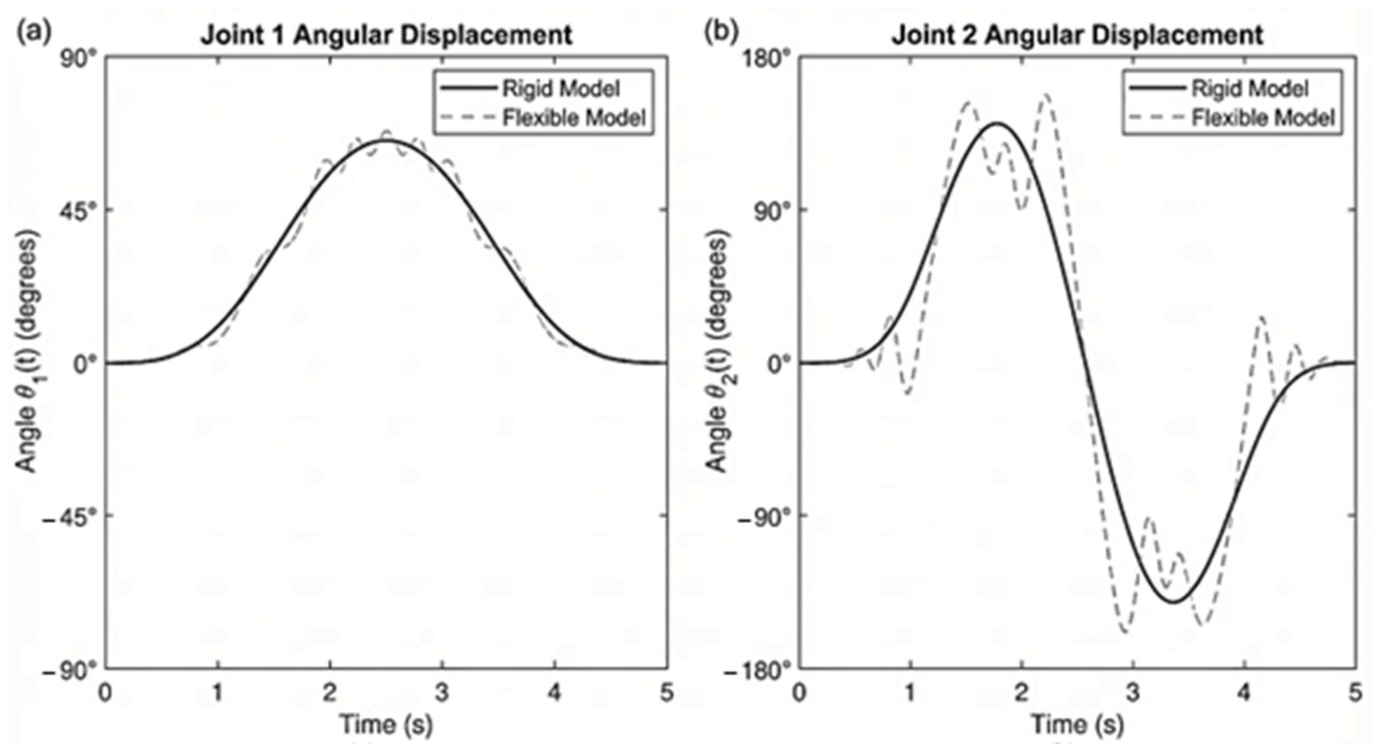
Initially, the angular displacement response of the two links for the rigid and flexible model was studied under harmonic excitation. As shown in Figure 3, the simulations of joint angles θ₁(t) and θ₂(t) for a 5 s period are presented.

Under harmonic excitation, the rigid model moves smoothly like a sine wave consistent with the imposed torque, while the flexible model moves with added wavering oscillation from bend motion. This additional wavering behavior arises from structural compliance governed by the bending stiffness, which is determined by the material properties and cross-sectional geometry listed in Table 1 (Section 2.2). The second joint response differs from the rigid-body prediction due to elastic deformation of the links, leading to additional oscillations and a delayed angular response relative to the applied excitation. The maximum angular deviation, 1.7° for joint 1 and 3.1° for joint 2, yields a tip deflection of 2.6 mm.

Following the termination of the harmonic torque excitation at $t=t_{off}$, the system response transitions from forced vibration to free decay. Under identical excitation conditions, the rigid-body model reached its steady forced-response amplitude within 0.48 s, whereas the flexible multibody model required 0.72 s to attenuate elastic oscillations and reach a steady response. The increased settling time in the flexible model is attributed to residual vibrations associated with elastic deformation of the links, represented through a reduced-order modal formulation retaining the first bending mode of each link. For the rigid-body formulation, the reported time corresponds to the transient duration required for the joint response to reach 95% of its steady forced-response amplitude. For the flexible model, settling time is defined as the time required for elastic vibration amplitudes to decay below 5% of their peak value.

3.2. Frequency-Domain Analysis and Mode Identification

The frequency-domain response of the end-effector displacement was obtained by applying a Fast Fourier Transform (FFT) to the steady-state portion of the simulated time-history signal. A Hanning window was used to reduce spectral leakage, and the frequency resolution was determined as Δf = 1/T, where T is the duration of the analyzed time window. The resulting spectrum provides insight into the dominant excitation and vibration components of the system.

The rigid-body model exhibits a single dominant peak at approximately 1.9 Hz, which corresponds directly to the applied excitation frequency and represents a purely forced response without internal structural dynamics. In contrast, the flexible multibody model exhibits several additional peaks in the frequency spectrum. These peaks arise from structural compliance introduced through the modal representation of the links. In the present formulation, each flexible link is represented using a reduced-order modal basis derived from linear beam theory. Specifically, one bending mode is retained for each link, introducing elastic coordinates that allow deformation of the structure during motion.

Although only one bending mode per link is retained, the coupled dynamics of the two-link manipulator generate multiple response peaks in the frequency spectrum of the end-effector displacement. These peaks represent coupled system vibration modes resulting from the interaction between rigid-body motion and elastic deformation. The dominant peaks were observed at approximately 17.6 Hz, 46.3 Hz, and 82.5 Hz, reflecting higher-frequency vibration components introduced by structural flexibility and dynamic coupling.

The first bending-mode frequency (17.6 Hz) is consistent with the analytical fundamental frequency of a cantilever beam with equivalent geometric and material properties, computed from Euler–Bernoulli beam theory. This agreement confirms that the reduced-order flexible formulation captures the dominant structural compliance of the links. While higher modes contribute less to overall displacement amplitude, they influence transient vibration content and settling behavior. Table 2 summarizes the dominant frequencies identified from the frequency spectrum along with the corresponding damping ratios used in the flexible model. Because the rigid-body model does not contain elastic degrees of freedom, it does not possess structural natural frequencies, and therefore, modal quantities are reported only for the flexible multibody formulation.

3.3. Effect of Mass and Stiffness Variation

To examine the influence of structural parameters on the dynamic response, a parametric study was performed by varying the material stiffness $E$ and link mass while maintaining constant geometric dimensions. The stiffness variation was implemented by scaling the Young’s modulus $E$, while the mass variation was introduced by scaling the material density $\rho$. In both cases, the link geometry (length, width, and thickness) remained unchanged to isolate the effects of stiffness and inertia.

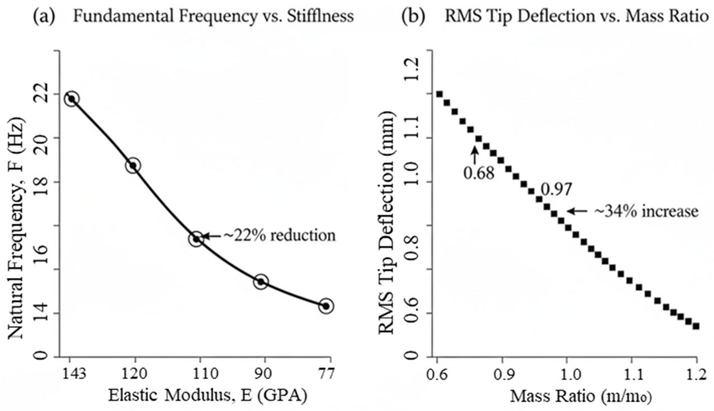
Figure 4a shows the variation in the fundamental bending frequency as a function of structural stiffness. When the Young’s modulus decreases from 110 GPa to 77 GPa (−30%), the natural frequency decreases by approximately 22%. This behavior is consistent with the classical relationship between bending stiffness and natural frequency of beam-like structures.

Figure 4b presents the variation in the RMS end-effector displacement as a function of the mass ratio. As the mass ratio decreases, the RMS vibration amplitude increases by approximately 34%. This increase reflects the greater susceptibility of lighter structures to dynamic excitation due to reduced inertial resistance. The results highlight the trade-off between structural stiffness and mass in flexible robotic systems. While reducing structural mass is desirable for lightweight design and improved actuator efficiency, excessive mass reduction may lead to increased vibration amplitudes and reduced dynamic stability. In the case of metallic structures manufactured with additive processes, the weight reduction in these components can be achieved mainly through the use of topology optimization and lattice infills. The results suggest that one should apply multi-objective optimization strategies for balancing stiffness, mass and damping, not mass minimization.

3.4. Comparative Dynamic Performance

Table 3. Summary of comparative dynamic metrics.

Metric	Rigid Model	Flexible Model	Remarks
Tip deflection amplitude (mm)	0.00	2.6	Elastic deformation present only in flexible model
Response rise time (s)	0.48	NA	Time to reach 95% of steady forced response
Settling time (s)	NA	0.72	Defined by decay of elastic oscillations
Peak angular error (°)	0.0	3.1	Relative to rigid kinematic response
RMS vibration amplitude (mm)	0.00	0.91	Vibration-induced displacement

presents a side-by-side comparison of the main performance metrics for the rigid and flexible models. Metrics associated with elastic vibration, such as settling time and RMS vibration amplitude, are defined only for the flexible multibody formulation, as the rigid-body model does not include elastic degrees of freedom.

These results quantitatively show that the flexible model induces measurable dynamic performance degradation, in particular, speed response and position accuracy. The observed trajectory deviation magnitude is directly influenced by the adopted Young’s modulus and link cross-sectional dimensions. Even minor deflections at the millimeter level can cause significant errors in the end-effector trajectory during fine manipulation. Also, the torque input and angular displacement’s phase lag imply that flexibility may change control bandwidth requirements. A stiff model might wrongly suggest steady performance at some excitation frequencies that, in reality, excite the flexible structure’s resonance.

3.5. Discussion and Implications

All of the results confirm that rigid-body approximations are inadequate for predicting the dynamic response of metal 3D-printed robotic mechanisms in which slender and lightweight links have significant compliance. Flexible modeling reveals dynamic modes not evident in rigid formulations and provides more realistic predictions of transient response, resonance, and control sensitivity in applications.

The results demonstrate that structural flexibility introduces coupling between rigid-body motion and elastic deformation through multibody kinematics. As the system configuration evolves over time, the elastic modal coordinates are excited by the joint motion, leading to the simultaneous participation of multiple bending modes in the dynamic response. For the studied configuration, flexibility introduced up to 3.1° angular deviation and 2.6 mm tip displacement relative to the rigid prediction, demonstrating that even moderate compliance can influence end-effector accuracy. The differences seen between results obtained with rigid versus flexible conditions are consistent with trends reported in experimental and numerical studies of flexible robotic manipulators [20].

This interaction results in a redistribution of vibrational energy among the retained modes, which influences transient response characteristics such as settling time and phase lag, even though the elastic behavior itself remains linear. With flexibility incorporated in the system, the design can be optimized for stiffness distribution, damping location, and control gain. From an engineering perspective, three key implications emerge: (i) flexible modeling significantly improves predictive fidelity for additively manufactured robotic structures, (ii) control strategies designed using rigid models risk instability when applied to flexible systems, and (iii) integrated simulation frameworks combining multibody dynamics, finite-element analysis, and optimization tools are essential for topology-aware stiffness tuning.

3.6. Future Prospects

Based on the comparative results presented in this study, flexible multibody modeling is vital in the accurate estimation of 3D-printed robotic dynamic mechanisms. One of the main issues for flexible multibody dynamics is that high-fidelity simulations are costly. The addition of each flexible body adds more degrees of freedom, increasing the size of system matrices and solution times. Even though the modal reduction techniques can relieve this problem, they require heavy pre-processing taking place in finite-element software. To address these limitations, future works should embed AI-driven surrogate models that replicate the behavior of complex simulations with a low computational cost. These surrogate models can approximate the nonlinear mapping between geometric, material and boundary parameters, and the dynamic responses, and are trained using datasets produced from parameterized dynamic simulations [21]. The use of hybrid physics-data systems could help with the fast prediction of dynamic responses for optimizations and adaptive control for flexible robots.

4. Conclusions

This study presented a comparative investigation of rigid and flexible multibody dynamic modeling for a 3D-printed two-link robotic mechanism, highlighting the limitations of rigid-body assumptions when applied to lightweight, additively manufactured structures. A reduced-order flexible multibody formulation was implemented to capture elastic deformation and modal dynamics, and the results were systematically compared with those obtained from a classical rigid-body model under identical excitation conditions. The principal findings can be summarized as follows:

• The flexible model displayed elastic deformations and vibrational modes not seen in the rigid model. Even slight compliance in the printed links resulted in a measurable deflection of about 2.6 mm and a phase lag between the applied joint torque and the angular displacement response, particularly at the distal joint.
• When the stiffness of the flexible links was reduced by 30%, the first natural frequency decreased by 22%, while the RMS tip vibration amplitude increased by 34%. These results indicate that lightweight structural design significantly influences the dynamic behavior of robotic manipulators and highlights the need for multi-parameter optimization in lightweight design.
• In contrast to rigid-body approaches, the flexible multibody model captured the effects of elastic damping and the interaction between rigid-body motion and elastic modes, which are critical for high-precision motion and dynamic stability.

The comparative framework presented in this work, therefore, provides a useful methodology for evaluating the impact of structural flexibility during the early stages of robotic mechanism design. While the present study provides a numerical comparison under controlled assumptions, experimental validation using a physical prototype would further quantify model fidelity and damping characterization. Such validation, together with the incorporation of process-induced material anisotropy, is identified as a direction for future work.