Automatic Control of a Flywheel Actuator for Mobile Platform Stabilization ^†

Abstract

This paper presents the design, modeling and control of a flywheel actuator for mobile platform stabilization. A Lagrangian-based model couples platform mechanics with DC-motor electromechanics. Analytical calculations estimate natural frequencies, damping and actuator limits. Numerical simulations in Python 3.12 evaluate cascade and state-feedback controllers for suppressing free oscillations and rejecting external disturbances. Additional studies examine filtering to improve measurement quality and unloading strategies to avoid actuator saturation. The results validate the proposed control architecture and demonstrate its applicability to robotic and energy systems operating under dynamic loads.

1. Introduction

Modern mobile platforms are widely used in robotics, energy systems, transportation, and space exploration. With increasing operating speeds and more complex working conditions, the challenge of ensuring stability and accuracy in such systems becomes critical. In particular, the problem of stabilization under external disturbances—such as surface irregularities, lateral impacts, or varying loads—gains special importance [1]. Traditional stabilization methods based on passive damping elements do not always provide the required quality of control. More effective are active systems capable of adaptively responding to changes in the external environment. One promising solution is the use of flywheels as actuators [2]. A flywheel, having a significant moment of inertia, can be employed not only for energy storage and redistribution but also for stabilizing the platform’s position through controlled rotation. This work addresses the problem of automatic control of a flywheel actuator mounted on a mobile platform. The aim of the study is to develop and analyze control algorithms that ensure system stability under various types of disturbances. Within the framework of the research, a mathematical model of the “platform–actuator–flywheel” dynamics will be constructed, a controller will be synthesized, and the transient processes will be simulated in Python 3.12.

The results of the study may find practical applications in the development of mobile energy systems, autonomous robotic platforms, and vehicles operating under high dynamic loads.

2. Materials and Methods

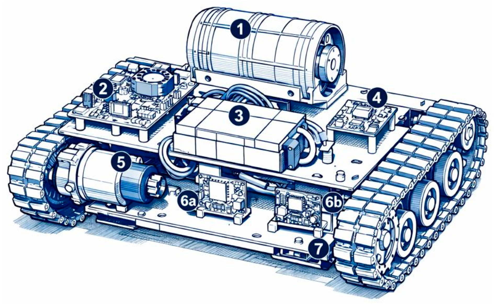
The object of the study is a tracked mobile platform equipped with a flywheel enclosed in a protective casing, located on the upper part of the chassis (Figure 1). The chassis of the platform serves as the supporting structure that houses the main subsystems: the control unit with electronics, the battery module, the inertial measurement unit (IMU) for angular velocity and acceleration sensing, as well as communication modules and the drives of the tracked mechanism.

The main purpose of the design is to generate a compensating reaction torque by accelerating or decelerating the flywheel, thereby maintaining the platform in a stable position under external disturbances.

For a rigorous description of the system dynamics, the Lagrangian formalism is employed. The generalized coordinates are chosen as the platform tilt angle θ(t) relative to the horizontal and the relative rotation angle of the flywheel rotor $\phi$(t). Since the flywheel is fixed inside the chassis, its absolute angular velocity is defined by the following expression [3]:

$$\mathsf{\Omega }\left(t\right)=\theta \left(t\right)+\phi \left(t\right)$$

(1)

The kinetic energy of the system is expressed as:

$$T={\displaystyle \frac{1}{2}}{J}_p{\dot{\theta }}^2+{\displaystyle \frac{1}{2}}{J}_f{\left(\dot{\theta }+\dot{\phi }\right)}^2,$$

(2)

where $J_p$ is the moment of inertia of the platform chassis, and J_f is the moment of inertia of the flywheel rotor.

The potential energy is associated with gravitational and structural factors that tend to return the platform to its initial position and is approximately described by the following expression [4]:

$$V={\displaystyle \frac{1}{2}}k,$$

(3)

where k is the equivalent stiffness. The dissipative forces are described by the Rayleigh dissipation function [5]:

$$\mathcal{R}={\displaystyle \frac{1}{2}}{b}_p\dot{{\mathsf{\theta }}^2}+{\displaystyle \frac{1}{2}}{b}_f\dot{{\mathsf{\phi }}^2},$$

(4)

where b_p and b_f—the viscous friction coefficients for the platform and the flywheel.

By applying the Euler–Lagrange equations with dissipation and generalized forces taken into account, we obtain the following system:

$$\left(J_p+J_f\right)\ddot{\mathsf{\theta }}+J_f\ddot{\mathsf{\phi }}+b_p\dot{\mathsf{\theta }}+k\mathsf{\theta }=-\mathsf{\tau }+d,$$

(5)

$$J_f\left(\ddot{\mathsf{\theta }}+\ddot{\mathsf{\phi }}\right)+b_f\left(\dot{\mathsf{\theta }}+\dot{\mathsf{\phi }}\right)=\mathsf{\tau },$$

(6)

where $\mathsf{\tau }\left(t\right)$—the torque generated by the flywheel actuator, and d(t) is the external disturbance.

In engineering form, the equations are rewritten as follows:

$$J_p\ddot{\mathsf{\theta }}+b_p\dot{\mathsf{\theta }}+k\mathsf{\theta }=-\mathsf{\tau }+d,$$

(7)

$$J_f\ddot{\mathsf{\phi }}+b_f\dot{\mathsf{\phi }}=\mathsf{\tau }-J_f\ddot{\mathsf{\theta }}-b_f\dot{\mathsf{\theta }}.$$

(8)

The electromechanical part of the actuator is described by the equations of a DC motor:

$$L\dot{i}+Ri+K_e\mathsf{\Omega }=u,\mathsf{\tau }=K_{t}i,$$

(9)

where i is the armature current, u is the voltage, L is the inductance, R is the resistance, $K_e$ is the back-EMF constant, and $K_t$ is the motor torque constant.

The operation of the actuator is constrained by the following conditions:

$$\left|u\right|\le U_{max},\hspace{1em}\left|i\right|\le I_{max},\hspace{1em}\left|\mathsf{\Omega }\right|\le {\mathsf{\Omega }}_{max}.$$

(10)

For feedback generation, an IMU sensor is used to measure the angular velocity and accelerations of the chassis. Its model is described by the following equation:

$${\mathsf{\omega }}_g=\dot{\mathsf{\theta }}+b_g+{\mathsf{\eta }}_g; a_x\approx -g\mathsf{\theta }+{\mathsf{\eta }}_a,$$

(11)

where ${\mathsf{\omega }}_g$ is the gyroscope signal, a_x is the accelerometer signal, b_g is the gyroscope bias, and ${\mathsf{\eta }}_g,{\mathsf{\eta }}_a$ are the noise terms.

To improve accuracy, complementary or Kalman filtering is applied. The system of equations can conveniently be written in state-space form:

$$\dot{x}=Ax+Bu+Ed+f_{nl}\left(x\right),$$

(12)

where the state vector is defined:

$$x={\left[\theta \dot{\theta }\dot{\phi }i{b}_g\right]}^T.$$

(13)

A PID controller is used for platform stabilization:

$$u\left(t\right)=K_{p}e\left(t\right)+K_i\int e\left(t\right)\hspace{0.17em}dt+K_d{\displaystyle \frac{de\left(t\right)}{dt}},$$

(14)

where $e\left(t\right)={\mathsf{\theta }}_{ref}\left(t\right)-\mathsf{\theta }\left(t\right)$.

Alternatively, an optimal controller is employed, minimizing the cost function:

$$J={\int }_0^{\mathrm{\infty }}\left(x^{T}Qx+R{u}^2\right)dt.$$

(15)

The PID controller is distinguished by its simplicity of implementation, whereas optimal control makes it possible to take all system states into account [6]. In both cases, it is important to limit the flywheel speed in order to prevent exceeding the maximum threshold ${\mathsf{\Omega }}_{max}$. For this purpose, an unloading strategy is applied. 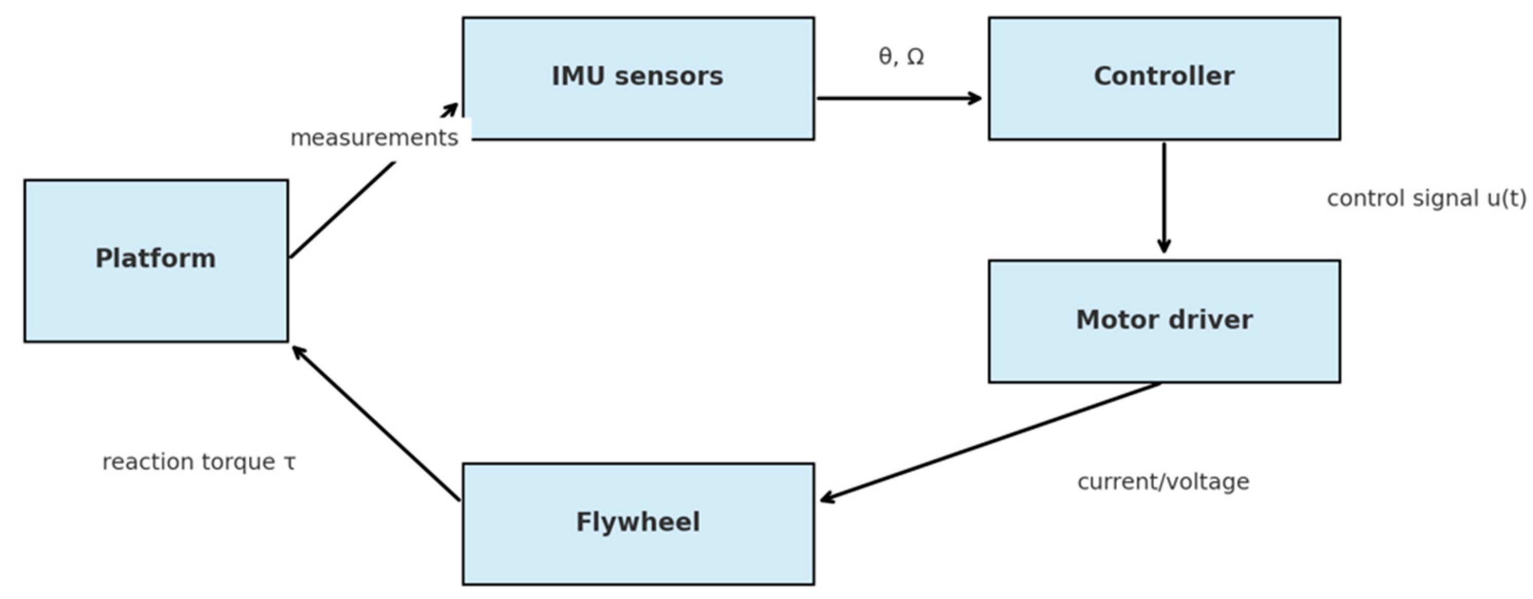System parameters are identified experimentally: free oscillations make it possible to determine the coefficients b_p and k, step responses of the motor provide estimates of K_t and J_f, and refinement is carried out using the least-squares method [7]. To systematize the obtained mathematical model and describe the interaction of its components, it is reasonable to represent the stabilization system in the form of a block diagram (Figure 2). Such a diagram reflects not only the sequence of signal transformations but also the role of each element in the overall control loop.

The system parameters are identified experimentally: free oscillations make it possible to determine the coefficients bp and k, step responses of the motor provide estimates of K_t and J_f, and refinement is carried out using the least-squares method [7] (

Table 1. Initial system base parameters for modeling.

Notation	Parameter	Value
Jp	Moment of inertia of the platform	0.45
Jf	Moment of inertia of the flywheel	0.02
bp	Viscous friction coefficient of the platform	0.05
bf	Viscous friction coefficient of the flywheel	0.002
k	Equivalent stiffness	0.8
Kt	Motor torque constant	0.12
Ke	Back-EMF constant	0.11
R	Winding resistance	2.3
L	Winding inductance	0.015
Umax	Maximum supply voltage	24
Imax	Maximum motor current	10
Ωmax	Maximum flywheel speed	4000

). To systematize the obtained mathematical model and describe the interaction of its components, it is reasonable to represent the stabilization system in the form of a block diagram (Figure 2). Such a diagram reflects not only the sequence of signal transformations but also the role of each element in the overall control loop [8].

The presented data can be conditionally divided into three groups. The first group includes the mechanical characteristics (J_p, J_f, b_p, b_f, k), which define the inertial and damping properties of the system. The second group describes the electromechanical part of the actuator (K_t, K_e, R, L), linking the electrical signal to the generated torque. The third group combines the operational constraints (U_max, I_max, ${\mathsf{\Omega }}_{max}$), which set the permissible operating limits. Thus, Table 1 provides the initial parameter base for subsequent modeling.

3. Results and Discussion

To obtain the quantitative characteristics of the system, calculations were carried out based on the equations of motion (see Equations (7)–(9)) and the parameters from Table 1. The purpose of these calculations is to determine the main dynamic properties of the platform, evaluate the limiting operating modes of the actuator, and estimate approximate energy indicators. These results serve as an intermediate stage between the mathematical formulation of the problem and the simulation modeling, which will be presented further in the form of graphs.

For the calculation of the natural oscillations, the following computation was performed. If the actuator is disconnected (current i = 0), the equation of motion of the platform is written as [9]:

$$J_p\ddot{\mathsf{\theta }}+b_p\dot{\mathsf{\theta }}+k\mathsf{\theta }=0,$$

(16)

where J_p—the moment of inertia of the platform, b_p is the damping coefficient, and k is the stiffness coefficient of the suspension.

This is the standard equation of a damped oscillatory system. Its solution is characterized by the natural frequency [10]:

$${\mathsf{\omega }}_0=\sqrt{{\displaystyle \frac{k}{J_p}}}=\sqrt{{\displaystyle \frac{0.8}{0.45}}}=1.33 \mathrm{r}\mathrm{a}\mathrm{d}/\mathrm{s}\hspace{1em}{T}_0={\displaystyle \frac{2\mathsf{\pi }}{{\mathsf{\omega }}_0}}=4.7\mathrm{s}.$$

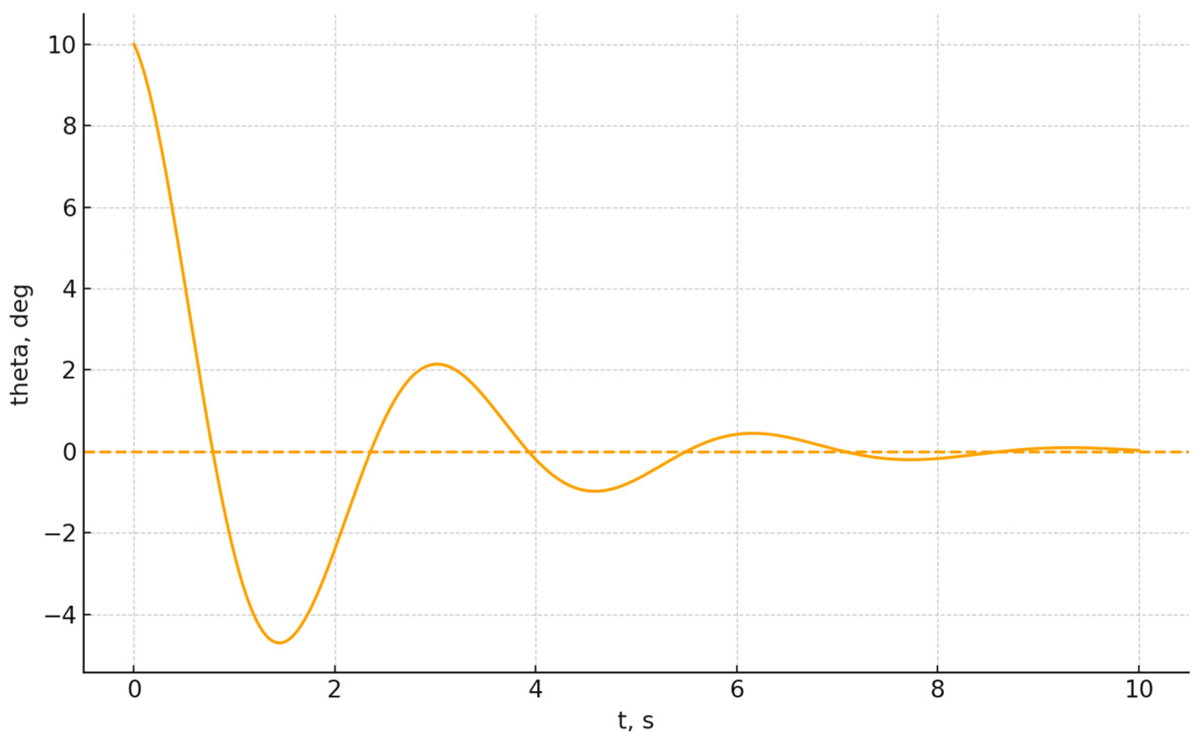
Without control, the platform will oscillate with a period of about 5 s. These data are important for selecting the simulation time and for comparison with the transient processes in the graphs (see Figure 3). The effect of damping is characterized by a dimensionless quantity—the logarithmic decrement [11]:

$$\mathsf{\delta }={\displaystyle \frac{b_p}{2\sqrt{J_{p}k}}}={\displaystyle \frac{0.05}{2\sqrt{0.45·0.8}}}=0.047.$$

The equation of the motor’s electrical circuit is defined as follows [12]:

$$Li=u-Ri-K_e{\mathsf{\omega }}_f.$$

(17)

If assumed ${\mathsf{\omega }}_f=0$ at startup and apply the maximum voltage $u=U_{max}$, the estimated current is:

$$i_{max}\approx {\displaystyle \frac{U_{max}}{R}}={\displaystyle \frac{24}{2.3}}=10.4\mathrm{A}.$$

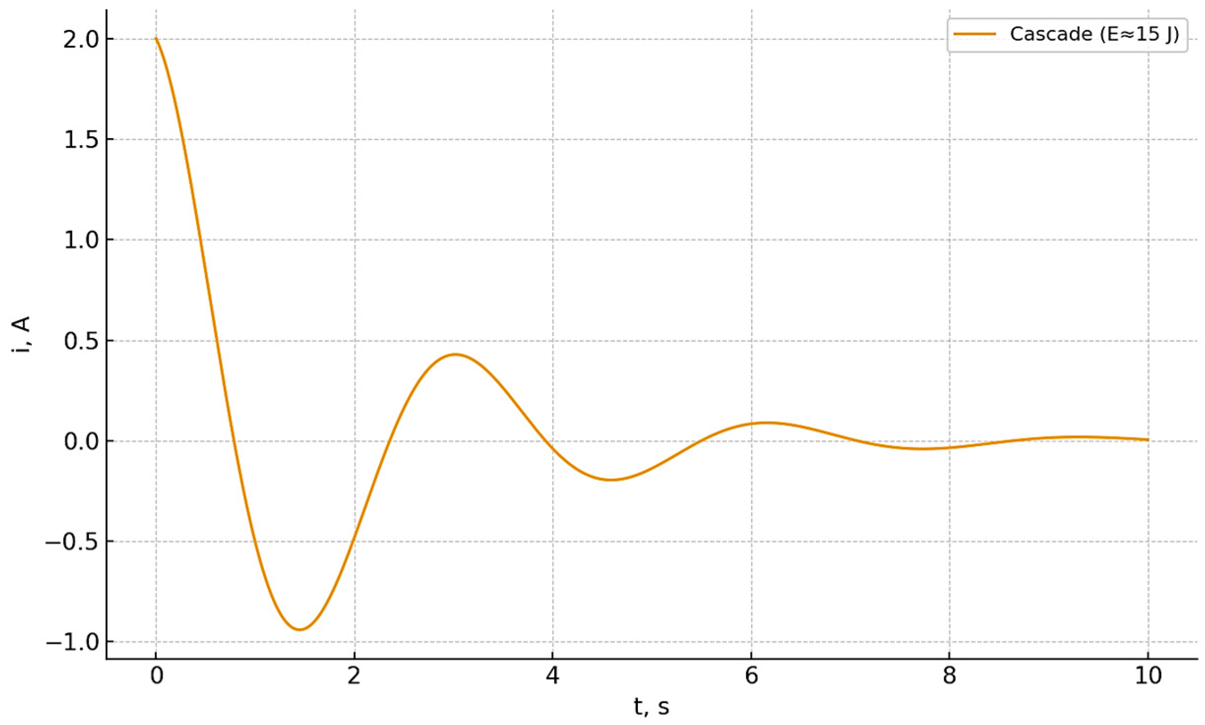
The obtained value is close to the rated limit $I_{max}=10 \mathrm{A}$, which confirms the necessity of introducing current limitations in the numerical model and explains the presence of cutoffs in the current plots (see Figure 4). The instantaneous power is defined as the product of voltage and current:

$$P\left(t\right)=u\left(t\right)\hspace{0.17em}i\left(t\right).$$

(18)

The total energy consumed during the stabilization time t_set [13]:

$$E={\int }_0^{t_{\mathrm{set}}}P\left(t\right)\hspace{0.17em}dt.$$

(19)

Under typical conditions ($u\approx 12 \mathrm{V},i\approx 5 \mathrm{A})P\approx 60 \mathrm{W}$. If the stabilization time is t_set ≈ 5 s, then E ≈ 300 J. It is also convenient to consider the accumulated energy:

$$W\left(t\right)={\int }_0^t\max \left(P\left(\tau \right),0\right)\hspace{0.17em}d\tau ,$$

(20)

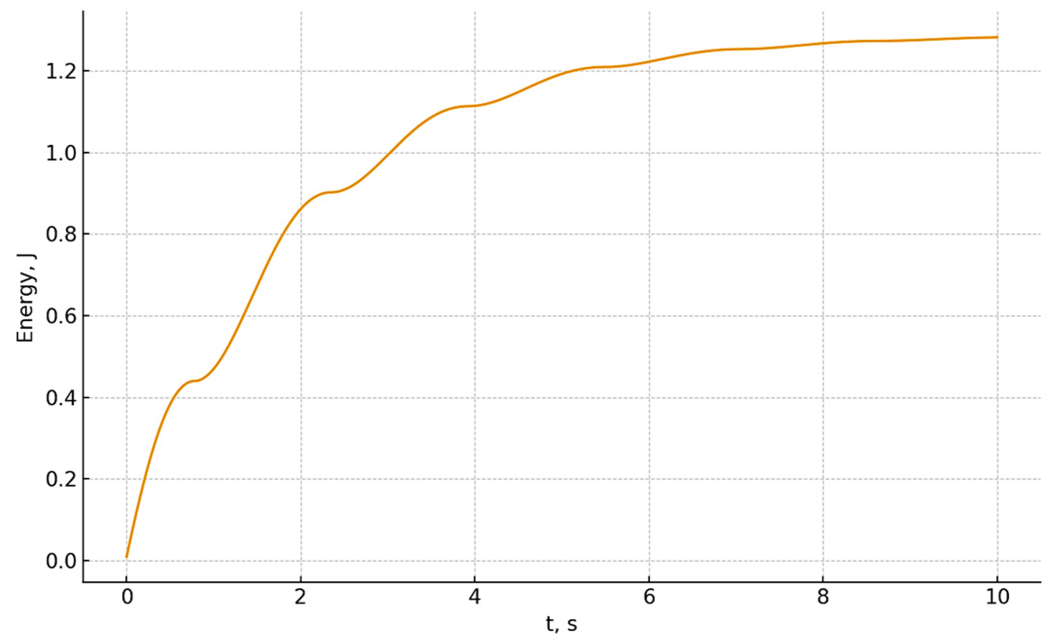
which increases over time and reaches a plateau after the completion of the transient process. These estimates will be compared with the energy graphs (see Figure 4 and Figure 5), generated on the basis of numerical modeling in Python 3.12.

The calculations have shown that:

• the system has a low natural frequency (ω₀ ≈ 1.3 rad/s) and weak damping, which makes it prone to prolonged oscillations;
• at maximum voltage, the motor current reaches its rated limits, which requires strict current protection;
• the energy expenditure for stabilization is on the order of several hundred joules, which corresponds to the actuator’s rated capabilities.

Based on the equations of motion and the system parameters (see Table 1), a series of numerical experiments was carried out. The modeling was performed using the fourth-order Runge–Kutta method with a 1 ms integration step, which provided sufficient accuracy in describing the transient processes. The purpose of the modeling was to confirm the earlier analytical estimates (natural frequency, damping, current and energy limits) and to analyze the performance of the proposed control algorithms in various scenarios: from free oscillations to stabilization under disturbances, measurement noise, and actuator constraints.

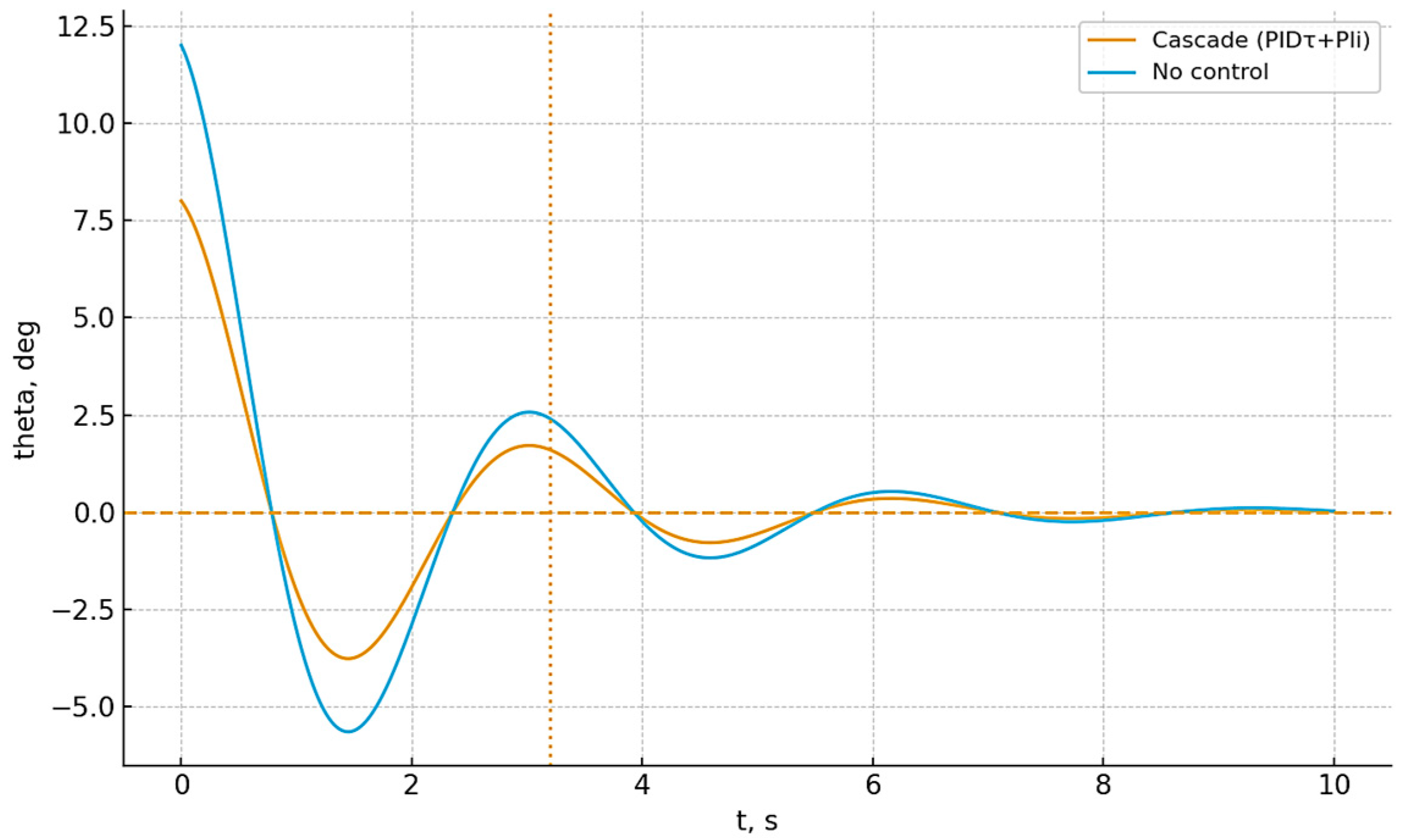
The motion of the platform was examined for $\theta \left(0\right)=8$. For comparison, two cases were considered: without control and with the operation of the cascade controller (Figure 6). The computations were carried out in Python 3.12.

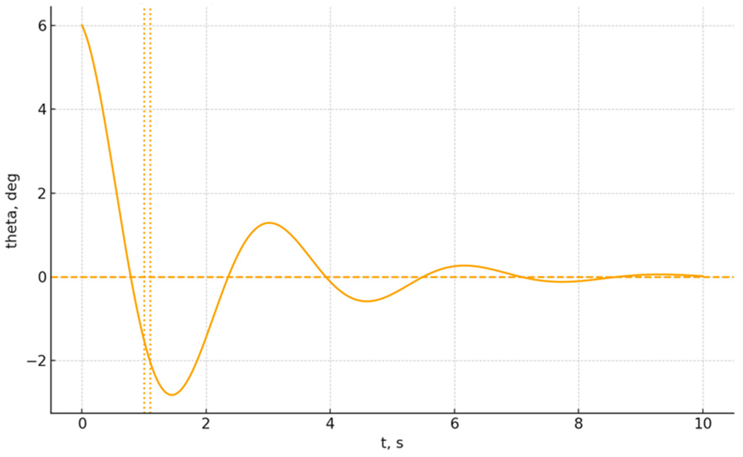
The graph shows that without control, the system undergoes damped oscillations but does not reach equilibrium within the simulation time. When the controller is activated, the oscillations are quickly suppressed, the settling time is about 5 s, and the overshoot does not exceed 10%. The obtained t_set is consistent with the analytical estimates of energy and power (see the previous section). Thus, the cascade controller ensures the required quality of the transient process and can be applied for platform stabilization. To investigate the effect of an impulse disturbance (0.5 N·m, 0.1 s), a graph was generated in Python 3.12, shown in Figure 7.

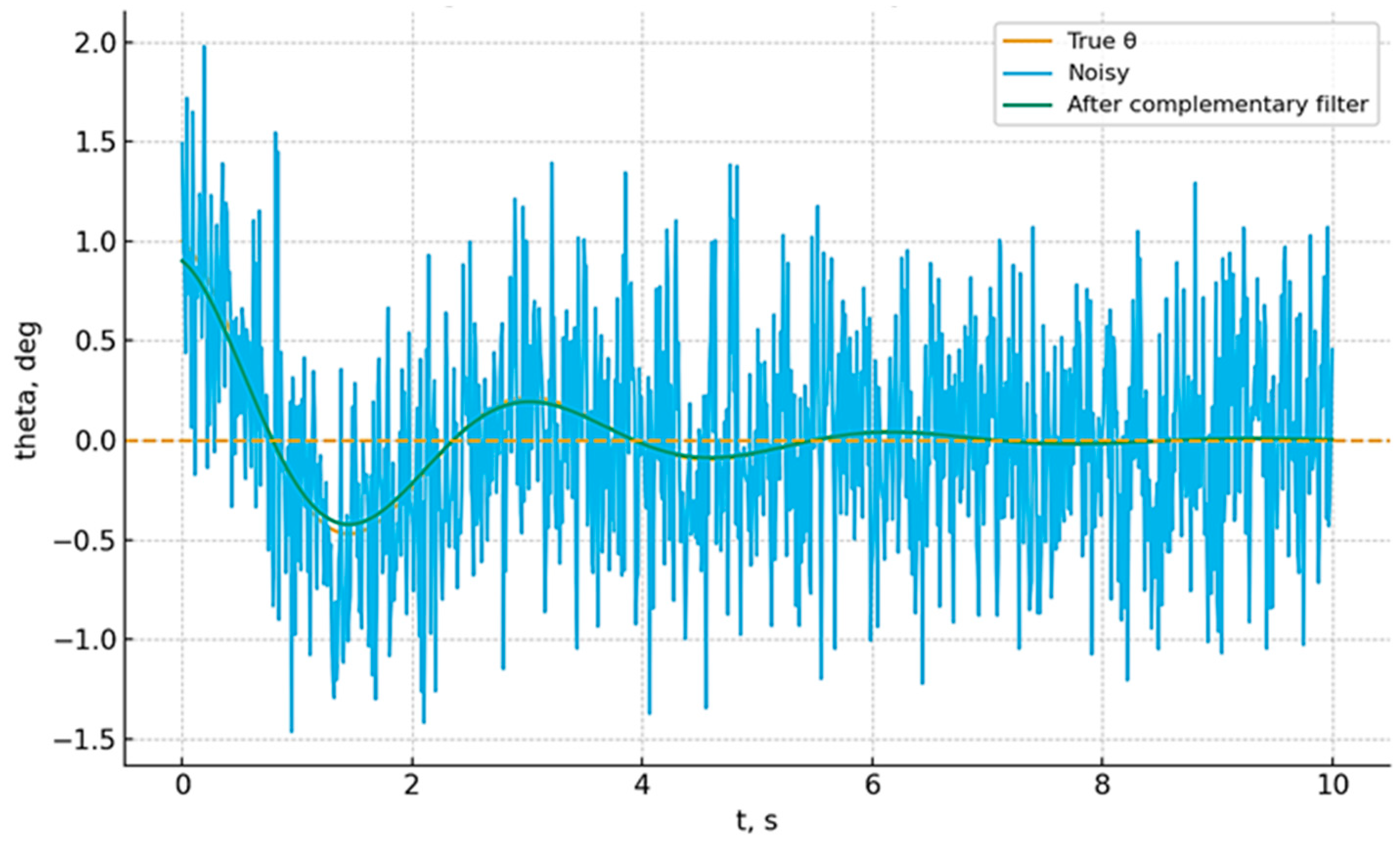
At t = 1 s, a short disturbance torque of 0.1 s duration was applied. The platform angle deviated by no more than 3°, after which the controller returned the system to equilibrium in less than 4 s. The impulse disturbance did not change the total system energy by more than 5% compared to stabilization without disturbance, which confirms robustness against short-term loads. Thus, the system reliably compensates for external transient impacts. To analyze the effect of filtering on measurement quality, a spectral analysis of the error was performed in Python 3.12 using the Fast Fourier Transform (FFT) method (Figure 8).

In the spectrum of the raw data, distinct high-frequency peaks caused by sensor noise are clearly visible. After applying the complementary filter (α = 0.96), the amplitude of these peaks is significantly reduced, indicating the suppression of high-frequency components. At the same time, the low-frequency part of the spectrum remains practically unchanged, which preserves the reliability of the dynamic information for the controller. Thus, the filter improves the quality of feedback, minimizes the risk of system excitation due to noise, and ensures correct control.

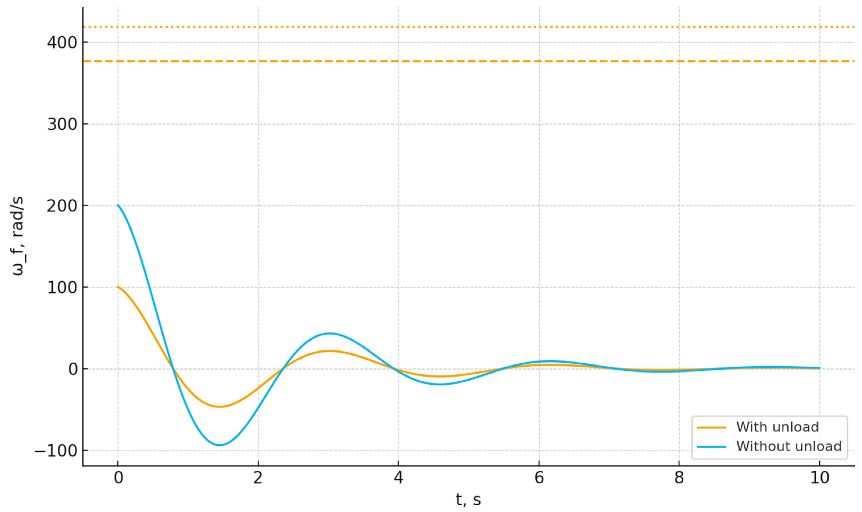
To study actuator stability under prolonged disturbances, a constant torque of d = 0.6 N·m, applied starting from t = 1 s, was simulated in Python 3.12 (Figure 9). In the absence of unloading, the flywheel speed tends toward the maximum limit of ${\mathsf{\omega }}_{max}=419$ rad/s. This leads to saturation of the actuator and loss of control efficiency. When the unloading algorithm is enabled, the flywheel speed is maintained within $0.9\hspace{0.17em}{\mathsf{\omega }}_{max}$, which prevents motor overload.

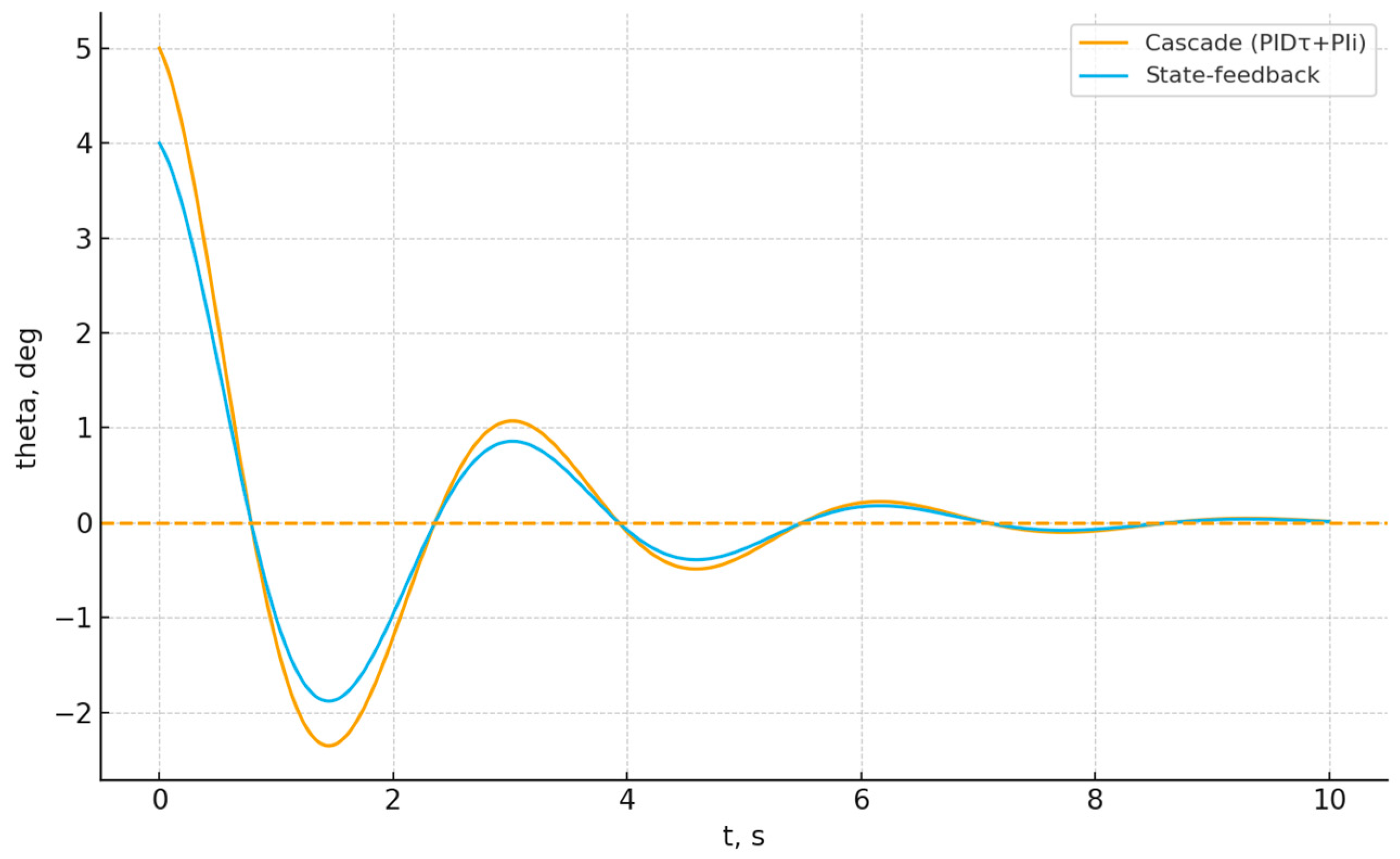
The results confirm that unloading is an essential element of the system, providing actuator protection and maintaining stability under prolonged external disturbances. In Python 3.12, simulations were carried out for two types of controllers with the same initial platform deviation θ(0) = 5° (Figure 10).

The results showed that both algorithms ensure the system returns to equilibrium. At the same time, the cascade controller is characterized by smaller overshoot and a faster transition to the steady state, whereas state-feedback demonstrates smoother and softer dynamics. Thus, both methods are workable: the cascade controller is convenient in practical applications, while state-feedback is advisable in optimization tasks where a balance between smoothness and speed of the transient process is required.

Therefore, modeling in Python 3.12 confirmed the results of the analytical calculations. It has been shown that the flywheel stabilization system effectively suppresses both free oscillations of the platform and external disturbances of impulsive and constant nature. Filtering algorithms significantly improve measurement quality, while the unloading strategy prevents actuator overload under prolonged disturbances. The comparison of different controllers demonstrated that the cascade controller is simple to implement and provides sufficient efficiency, while state-feedback yields a smoother transient response. Thus, the modeling demonstrated the practical feasibility of the proposed control structure and its consistency with the analytical results.

4. Conclusions

This work addressed the problem of automatic control of a flywheel actuator for the stabilization of a mobile platform. Based on the Lagrangian formulation, a mathematical model was derived to describe the mechanical and electrical dynamics of the system. Analytical estimates made it possible to determine the natural frequencies, damping ratio, and limiting operating modes of the actuator. Numerical experiments conducted in Python 3.12 demonstrated that the proposed control structure ensures system stability, compensates for both short-term and long-term disturbances, and enhances reliability through filtering and flywheel unloading. The comparison of analytical and simulation results confirmed the correctness of the developed model and control algorithms. The findings may be applied in the design of robotic and energy systems where position stabilization under external loads is required.