Partial Differential Equations of Motion for a Single-Link Flexible Manipulator ^†

Abstract

Robot manipulators have played an enormous role in the industry during the twenty-first century. Due to the advances in materials science, lightweight manipulators have emerged with low energy consumption and positive economic aspect regardless of their complex mechanical model and control techniques problems. This paper presents a dynamic model of a single link flexible robot manipulator with a payload at its free end based on the Euler–Bernoulli beam theory with a complete second-order deformation field that generates a complete second-order elastic rotation matrix. The beam experiences an axial stretching, horizontal and vertical deflections, and a torsional deformation ignoring the shear due to bending, warping due to torsion, and viscous air friction. The deformation and its derivatives are assumed to be small. The application of the extended Hamilton principle while taking into account the viscoelastic internal damping based on the Kelvin–Voigt model expressed by the Rayleigh dissipation function yields both the boundary conditions and the coupled partial differential equations of motion that can be decoupled when the manipulator rotates with a constant angular velocity. Equations of motion solutions are still under research, as it is required to study the behavior of flexible manipulators and develop novel ways and methods for controlling their complex movements.

1. Introduction

The focus of robotics research in the last decade has been on building lightweight manipulators due to their low energy consumption despite their complex mechanical models and control systems. Lightweight manipulators are considered flexible manipulators that suffer from flexural effects, which leads to growing interest toward modeling and control architecture of such systems. In general, the research is restricted to single-link flexible manipulator [1] due to the intricacy of serial link flexible manipulators. In the literature, the single link is usually modeled by one deformation parameter [2], and the kinematics of the Euler–Bernoulli beam is usually approached by the assumed traditional deformation field that cannot allow having an orthogonal elastic rotation matrix to the second-order. For this article, the deformations and their partial derivatives are assumed to be small. The kinematic model described in Section 2.1 is based on the complete second-order deformation field [3]. Section 2.2 presents the dynamics model that includes the kinetic energy and potential energy of the system that is composed of gravitational and strain potential energies due to gravity and elasticity. Section 2.3 takes into account the Rayleigh dissipation function due to motor friction and the viscoelastic internal damping based on the Kelvin–Voigt model. Section 2.4 gives the motion equations using the extended Hamilton principle that yields four partial differential equations satisfied by the deformation variables and seven boundary conditions. Lastly, Section 3 deals with the decoupling of partial differential equations in a particular case which allows small simplifications of the equations.

2. Mechanical Modeling

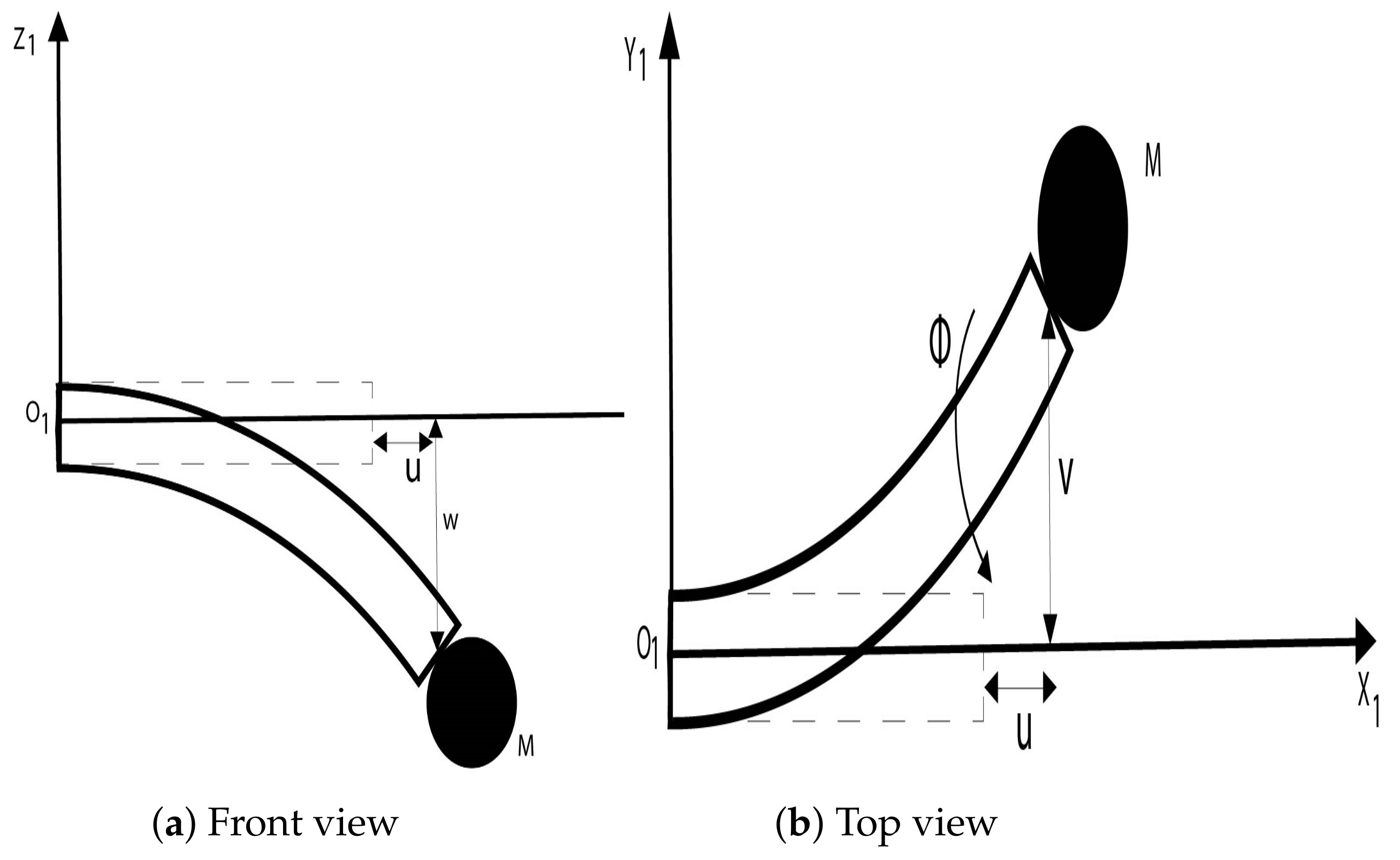
The system consists of a base subjected to an applied torque $T_{mot}$ by a motor, a flexible link modeled as an Euler–Bernoulli beam with a circular cross-section with radius R and length L, and a payload with mass $m_p$ and inertia matrix $I_p$ at the free end of the link. The beam is subjected to an axial stretching $u(x,t)$, a horizontal deflection $v(x,t)$, a vertical deflection $w(x,t)$ and a torsional deformation $\varphi (x,t)$, as shown in (Figure 1a,b) where the axis $Z_1$ is perpendicular to the ground. The beam deformations and their partial derivatives are assumed to be small, and shear due to bending, warping due to torsion, and air viscous friction are neglected. To simplify the notation, $u(x,t)$, $v(x,t)$, $w(x,t)$, $\varphi (x,t)$,$\frac{d}{dt}(.)$, $\frac{d}{dx}(.)$ are denoted by u, v, w, $\varphi$, $\dot{(.)}$ and ${(.)}^{\prime }$ respectively.

2.1. Kinematics

Let ${\mathcal{R}}_0$ be an inertial frame with origin $O_0$, ${\mathcal{R}}_1$ a frame attached to the motor with origin $O_1$ that coincides with $O_0$, and ${\mathcal{R}}_{dm}$ a frame attached to the cross-section of mass dm whose axes are parallel to those of ${\mathcal{R}}_1$ before deformation and whose origin $O_{dm}$ is the center of the cross-section that is at a distance x from $O_1$ along the neutral axis of the link before deformation. The rotation matrix of ${\mathcal{R}}_1$ relative to ${\mathcal{R}}_0$[4] is ${}^0{R}_1=R_{Z_0,\theta }$ which means the frame $R_1$ rotates by an angle $\theta$ of about $Z_0$.

The position of $O_{dm}$ relative to ${\mathcal{R}}_1$ expressed in ${\mathcal{R}}_1$ after deformation [3] expressed by:

$${}^1\overrightarrow{O_1{O}_{dm}}={[x+u-\frac{1}{2}{\int }_0^x({v^{\prime }}^2+{w^{\prime }}^2)ds,v,w]}^T$$

(1)

The rotation matrix of ${\mathcal{R}}_{dm}$ relative to ${\mathcal{R}}_1$ after deformation [3] is:

$${}^1{R}_{dm}=\left[\begin{array}{ccc}1-\frac{1}{2}({v^{\prime }}^2+{w^{\prime }}^2)& -v^{\prime }+u^{\prime }{v}^{\prime }-w^{\prime }\varphi & -w^{\prime }+u^{\prime }{w}^{\prime }+v^{\prime }\varphi \\ v^{\prime }-u^{\prime }{v}^{\prime }& 1-\frac{1}{2}({v^{\prime }}^2+{\varphi }^2)& -\varphi -\frac{1}{2}{v}^{\prime }{w}^{\prime }\\ w^{\prime }-u^{\prime }{w}^{\prime }& \varphi -\frac{1}{2}{v}^{\prime }{w}^{\prime }& 1-\frac{1}{2}({w^{\prime }}^2+{\varphi }^2)\end{array}\right]$$

(2)

${}^1{R}_{dm}$ is verified to be orthogonal to the second-order of Taylor expansion in the deformation variables. Let P be a point of the cross-section with (x, y, z) its coordinates relative to ${\mathcal{R}}_1$ before deformation. The position of P relative to ${\mathcal{R}}_1$ expressed in ${\mathcal{R}}_1$ after deformation [4] is

$${}^1\overrightarrow{O_{1}P}{=}^1\overrightarrow{O_1{O}_{dm}}+{}^1{R}_{dm}{}^{dm}\overrightarrow{O_{dm}P}$$

where ${}^{dm}\overrightarrow{O_{dm}P}={[0,y,z]}^T$ and ${}^0\overrightarrow{O_{0}P}={}^0{R}_1{}^1\overrightarrow{O_{1}P}$.

Let ${\mathcal{R}}_2$ be a frame attached to the free end of the link whose origin is $O_2$ and obtained from ${\mathcal{R}}_{dm}$ by replacing x by L (for example v(x,t) at x=L becomes $v(L,t)$, shortened $v_L$). If the position of the center of mass C of the payload relative to ${\mathcal{R}}_2$ expressed in ${\mathcal{R}}_2$ is ${}^2\overrightarrow{O_{2}C}={[c,0,0]}^T$, then the position of C relative to ${\mathcal{R}}_1$ expressed in ${\mathcal{R}}_1$ is given by:

$$\begin{array}{c}\hfill {}^1\overrightarrow{O_{1}C}={[L+u_L-\frac{1}{2}{\int }_0^L({v^{\prime }}^2+{w^{\prime }}^2)ds+c\left(1-\frac{1}{2}({{vL}^{\prime }}^2+{{wL}^{\prime }}^2)\right),v_L+c(v_L^{\prime }-u_L^{\prime }{v}_L^{\prime }),w_L+c(w_L^{\prime }-u_L^{\prime }{w}_L^{\prime })]}^T\end{array}$$

(3)

Since ${}^1\overrightarrow{O_{1}C}={}^1\overrightarrow{O_1{O}_2}+{}^1{R}_2{}^2\overrightarrow{O_{2}C}$, and ${}^1{R}_2$ is deduced from $1R_{dm}$ by replacing x by L; hence, ${}^0\overrightarrow{O_{0}C}={}^0{R}_1{}^1\overrightarrow{O_{1}C}$. The angular velocity of ${\mathcal{R}}_1$ relative to ${\mathcal{R}}_0$ expressed in ${\mathcal{R}}_0$ is ${}^0\overrightarrow{{\Omega }_{1/0}}={[0,0,\dot{\theta }]}^T$. The angular velocity of ${\mathcal{R}}_{dm}$ relative to ${\mathcal{R}}_1$ expressed in ${\mathcal{R}}_1$ [4] is found from the following matrix

$$S={}^1{\dot{R}}_{dm}{}^1{R}_{dm}^T=\left[\begin{array}{ccc}0& -{\omega }_z& {\omega }_y\\ {\omega }_z& 0& -{\omega }_x\\ -{\omega }_y& {\omega }_x& 0\end{array}\right]$$

Hence,

$${}^1\overrightarrow{{\Omega }_{dm/1}}={[{\omega }_x,{\omega }_y,{\omega }_z]}^T$$

The Taylor expansion of ${}^1\overrightarrow{{\Omega }_{dm/1}}$ to the second-order in the deformation variables and after simplification gives:

$$\begin{array}{cccccc}\hfill {\omega }_x& \approx \dot{\varphi }+\frac{1}{2}(v^{\prime }{\dot{w}}^{\prime }-{\dot{v}}^{\prime }{w}^{\prime })\hfill & \hspace{1em}\hspace{1em}\hfill {\omega }_y& \approx -{\dot{w}}^{\prime }+{\dot{u}}^{\prime }{w}^{\prime }+u^{\prime }{\dot{w}}^{\prime }+v^{\prime }\dot{\varphi }\hfill & \hspace{1em}\hspace{1em}\hfill {\omega }_z& \approx {\dot{v}}^{\prime }-{\dot{u}}^{\prime }{v}^{\prime }-u^{\prime }{\dot{v}}^{\prime }+\dot{\varphi }{w}^{\prime }\hfill \end{array}$$

(4)

Hence, the angular velocity of ${\mathcal{R}}_{dm}$ relative to ${\mathcal{R}}_0$ expressed in ${\mathcal{R}}_0$ is given by:

$${}^0\overrightarrow{{\Omega }_{dm/0}}={}^0\overrightarrow{{\Omega }_{1/0}}+{}^0{R}_1{}^1\overrightarrow{{\Omega }_{dm/1}}$$

The gravity vector is represented in ${\mathcal{R}}_0$ by: ${}^0\overrightarrow{g}={[0,0,-g]}^T$.

2.2. Dynamics

2.2.1. Kinetic Energy

The kinetic energy T of the system is the sum of kinetic energies: $T_B$ of the base, $T_l$ of the flexible link and $T_p$ of the payload. Where $T_B=\frac{1}{2}{I}_B{\dot{\theta }}^2$, with $I_B$ is the base inertia about the $Z_0$ axis. The kinetic energy of the link [5] is given by:

$$T_l=\frac{1}{2}{\int \int \int }_{V}v{(P/0)}^{2}dm=\frac{1}{2}{\int }_{z=-R}^R{\int }_{y=-\sqrt{R^2-z^2}}^{\sqrt{R^2-z^2}}{\int }_{x=0}^L\rho v{(P/0)}^{2}dxdydz$$

(5)

Since the beam cross-section is circular, $y^2+z^2=r^2,r\in [0,R]$ and the last triple integral is written [6] as:

$$T_l=\frac{1}{2}{\int }_{r=0}^R{\int }_{\gamma =0}^{2\pi }{\int }_{x=0}^L\rho v{(P/0)}^{2}rdrd\gamma dx$$

(6)

where $y=rcos\left(\gamma \right),z=rsin\left(\gamma \right)$. Therefore, the kinetic energy of the link linearized to the second-order and after simplifications is given by:

$$\begin{array}{cc}\hfill T_l& =\frac{\rho }{2}\{\pi R^2{\int }_0^L({\dot{u}}^2+{\dot{v}}^2+{\dot{w}}^2)dx+\frac{1}{4}\pi R^4{\int }_0^L({{\dot{v}}^{\prime }}^2+{{\dot{w}}^{\prime }}^2+2{\dot{\varphi }}^2)dx+{\dot{\theta }}^2[\frac{1}{3}\pi R^2{L}^3+\frac{1}{4}\pi R^{4}L+\pi R^2{\int }_0^L(u^2+v^2)dx+\hfill \\ & \frac{1}{4}\pi R^4{\int }_0^L{w^{\prime }}^{2}dx+2\pi R^2{\int }_0^{L}xudx-\frac{1}{2}\pi R^2{\int }_0^L(L^2-x^2)({v^{\prime }}^2+{w^{\prime }}^2)dx]+2\dot{\theta }[\pi R^2{\int }_0^{L}x\dot{v}dx-\hfill \\ & \frac{1}{4}\pi R^4{\int }_0^L(-{\dot{v}}^{\prime }+{\dot{u}}^{\prime }{v}^{\prime }+u^{\prime }{\dot{v}}^{\prime }-2w^{\prime }\dot{\varphi })dx+\pi R^2{\int }_0^L(u\dot{v}-\dot{u}v)dx\left]\right\}\hfill \end{array}$$

(7)

The kinetic energy of the payload [7] is expressed by:

$$T_p=\frac{1}{2}\overrightarrow{{\Omega }_{p/0}}.I_p\overrightarrow{{\Omega }_{p/0}}+\frac{1}{2}{m}_{p}v{(C/0)}^2$$

(8)

where $I_p=\left[\begin{array}{ccc}{I}_1& I_4& I_5\\ I_4& I_2& I_6\\ I_5& I_6& I_3\end{array}\right]$ and $\overrightarrow{{\Omega }_{p/0}}$ is obtained from $\overrightarrow{{\Omega }_{dm/0}}$ by replacing x by L; hence, the expression of $T_p$ linearized to the second-order in the deformation variables is given by:

$$\begin{array}{cc}\hfill T_p& =\frac{1}{2}[I_1\left({\dot{\varphi }}_L^{2}cos{\left(\theta \right)}^2+{\dot{w}}_{L^{\prime }}^{2}sin{\left(\theta \right)}^2+2{\dot{\varphi }}_L{\dot{w}}_L^{\prime }cos\left(\theta \right)sin\left(\theta \right)\right)+I_2\left({\dot{\varphi }}_L^{2}sin{\left(\theta \right)}^2+{\dot{w}}_L^{\prime 2}cos{\left(\theta \right)}^2-2{\dot{\varphi }}_L{\dot{w}}_L^{\prime }cos\left(\theta \right)sin\left(\theta \right)\right)\hfill \\ & +I_3\left({\dot{\theta }}^2+{{\dot{v}}^{\prime }}_L^2+2\dot{\theta }({\dot{v}}_L^{\prime }-{\dot{u}}_L^{\prime }{v}_L^{\prime }-u_L^{\prime }{\dot{v}}_L^{\prime }+{\dot{\varphi }}_L{w}_L^{\prime })\right)+2I_4\left(({\dot{\varphi }}_L^2-{{\dot{w}}^{\prime }}_L^2)cos\left(\theta \right)sin\left(\theta \right)-{\dot{\varphi }}_L{\dot{w}}_L^{\prime }\left(2cos{\left(\theta \right)}^2-1\right)\right)+\hfill \\ & 2I_5\left(\dot{\theta }\left(\left({\dot{\varphi }}_L+\frac{1}{2}(v_L^{\prime }{\dot{w}}_L^{\prime }-{\dot{v}}_L^{\prime }{w}_L^{\prime })\right)cos\left(\theta \right)-(-{\dot{w}}_L^{\prime }+{\dot{u}}_L^{\prime }{w}_L^{\prime }+u_L^{\prime }{\dot{w}}_L^{\prime }+v_L^{\prime }{\dot{\varphi }}_L)sin\left(\theta \right)\right)+{\dot{v}}_L^{\prime }{\dot{\varphi }}_{L}cos\left(\theta \right)+{\dot{v}}_L^{\prime }{\dot{w}}_L^{\prime }sin\left(\theta \right)\right)\hfill \\ & +2I_6\left(\dot{\theta }\left(\left({\dot{\varphi }}_L+\frac{1}{2}(v_L^{\prime }{\dot{w}}_L^{\prime }-{\dot{v}}_L^{\prime }{w}_L^{\prime })\right)sin\left(\theta \right)+(-{\dot{w}}_L^{\prime }+{\dot{u}}_L^{\prime }{w}_L^{\prime }+u_L^{\prime }{\dot{w}}_L^{\prime }+v_L^{\prime }{\dot{\varphi }}_L)cos\left(\theta \right)\right)+{\dot{v}}_L^{\prime }{\dot{\varphi }}_{L}sin\left(\theta \right)-{\dot{v}}_L^{\prime }{\dot{w}}_L^{\prime }cos\left(\theta \right)\right)]+\hfill \\ & \frac{1}{2}{m}_p[{\dot{u}}_L^2+{\dot{v}}_L^2+{\dot{w}}_L^2+c^2({{\dot{v}}^{\prime }}_L^2+{{\dot{w}}^{\prime }}_L^2)+2c({\dot{v}}_L{\dot{v}}_L^{\prime }+{\dot{w}}_L{\dot{w}}_L^{\prime })+{\dot{\theta }}^2(L^2+u_L^2+v_L^2+c^2(1-{w^{\prime }}_L^2)+2L[u_L-\frac{1}{2}{\int }_0^L({v^{\prime }}^2+{w^{\prime }}^2)ds+\hfill \\ & c\left(1-\frac{1}{2}({v^{\prime }}_L^2+{w^{\prime }}_L^2)\right)]+2c(u_L+v_L{v}_L^{\prime })-c{\int }_0^L({v^{\prime }}^2+{w^{\prime }}^2)ds)+2\dot{\theta }(\left(L+c\right)\left({\dot{v}}_L+c({\dot{v}}_L^{\prime }-{\dot{u}}_L^{\prime }{v}_L^{\prime }-u_L^{\prime }{\dot{v}}_L^{\prime })\right)+u_L({\dot{v}}_L+c{\dot{v}}_L^{\prime })-\hfill \\ & {\dot{u}}_L(v_L+c{v}_L^{\prime })\left)\right]\hfill \end{array}$$

(9)

2.2.2. Potential Energy

The potential energy V of the system is the sum of potential energies:$V_B$ of the base, $V_l$ of the flexible link and $V_p$ of the payload. The potential energy $V_B$ of the base which is its gravitational potential energy equals a constant $C_B$ because its mass center is fixed in the inertial frame ${\mathcal{R}}_0$ whose origin level is taken as reference $V_B=C_B$.The potential energy of the link is the sum of its gravitational potential energy and its strain energy:

$$V_l=V_{gravit}+V_{str}$$

(10)

$V_{gravit}$ is the gravitational potential energy of the link [7] that equals:

$$V_{gravit}=-{\int }_{r=0}^R{\int }_{\gamma =0}^{2\pi }{\int }_{x=0}^L\overrightarrow{g}\overrightarrow{O_{0}P}\rho rdrd\gamma dx=\rho g\pi R^2{\int }_{x=0}^{L}wdx$$

(11)

$V_{str}$ is the strain energy of the link [8] and it is the sum of strain energies due to different strains:

$$V_{str}=V_u+V_v+V_w+V_{\varphi }$$

(12)

The expressions of different strain energies [9] are:

$$\begin{array}{ccccc}\hfill V_u& =\frac{1}{2}\underset{V}{\int \int \int }E{u^{\prime }}^{2}dV=\frac{1}{2}\pi R^{2}E{\int }_0^L{u^{\prime }}^{2}dx\hfill & \hfill V_v& =\frac{1}{2}\underset{V}{\int \int \int }E{v^{″}}^2{y}^{2}dV=\frac{1}{8}\pi R^{4}E{\int }_0^L{v^{″}}^{2}dx\hfill & \hfill V_w=\frac{1}{2}\underset{V}{\int \int \int }E{w^{″}}^2{z}^{2}dV=\frac{1}{8}\pi R^{4}E{\int }_0^L{w^{″}}^{2}dx\\ & V_{\varphi }=\frac{1}{2}\underset{V}{\int \int \int }G{r}^2{{\varphi }^{\prime }}^{2}dV=\frac{1}{4}\pi R^{4}G{\int }_0^L{{\varphi }^{\prime }}^{2}dx\hfill \end{array}$$

where E and G are the young modulus and the shear modulus of the beam material respectively. The potential energy of the payload is its gravitational potential energy that equals:

$$V_p=-m_p\overrightarrow{g}\overrightarrow{O_{0}C}=m_{p}g\left(w_L+c(w_L^{\prime }-u_L^{\prime }{w}_L^{\prime })\right)$$

(13)

2.3. Rayleigh Dissipation Function

Rayleigh dissipation function $\mathcal{R}$ expresses the energy dissipated due to motor friction and internal damping effect of each deformation $(u,v,w,\varphi )$, the dissipation is based on the Kelvin–Voigt model [10], and can be expressed [11] as follows:

$$\mathcal{R}={\mathcal{R}}_{mot}+{\mathcal{R}}_u+{\mathcal{R}}_v+{\mathcal{R}}_w+{\mathcal{R}}_{\varphi }$$

(14)

where

$$\begin{array}{cccccc}\hfill {\mathcal{R}}_u& =\frac{1}{2}{\int \int \int }_V{\sigma }_u^d{\dot{ϵ}}_{u}dV=\frac{1}{2}\pi R^2{C}_X{\int }_{x=0}^L{{\dot{u}}^{\prime }}^{2}dx\hfill & \hfill {\mathcal{R}}_v& =\frac{1}{2}{\int \int \int }_V{\sigma }_v^d{\dot{ϵ}}_{v}dV=\frac{1}{8}\pi R^4{C}_Y{\int }_{x=0}^L{{\dot{v}}^{″}}^{2}dx\hfill & \hfill {\mathcal{R}}_w& =\frac{1}{2}{\int \int \int }_V{\sigma }_w^d{\dot{ϵ}}_{w}dV=\frac{1}{8}\pi R^4{C}_Z{\int }_{x=0}^L{{\dot{w}}^{″}}^{2}dx\hfill \\ \hfill {\mathcal{R}}_{\varphi }& =\frac{1}{2}{\int \int \int }_V{\tau }_{\varphi }^d{\dot{\gamma }}_{\varphi }dV=\frac{1}{4}\pi R^4{C}_{\Phi }{\int }_{x=0}^L{{\dot{\varphi }}^{\prime }}^{2}dx\hfill & \hfill {\mathcal{R}}_{mot}& =\frac{1}{2}{b}_m{\dot{\theta }}^2\hfill \end{array}$$

Since

$$|{ϵ}_u|=|u^{\prime }|,{\sigma }_u^d=C_X{\dot{ϵ}}_u,|{ϵ}_v|=|y{v}^{″}|=|rcos\left(\gamma \right)v^{″}|,{\sigma }_v^d=C_Y{\dot{ϵ}}_v,$$

$$|{ϵ}_w|=|z{w}^{″}|=|rsin\left(\gamma \right)w^{″}|,{\sigma }_w^d=C_Z{\dot{ϵ}}_w,|{\gamma }_{\varphi }|=|r{\varphi }^{\prime }|and{\tau }_{\varphi }^d=C_{\Phi }{\dot{\gamma }}_{\varphi }.$$

2.4. Motion Equations

The extended Hamilton principle [12] is used to get motion equations and boundary conditions: $0={\int }_{t_1}^{t_2}(\delta T-\delta V+T_{mot}\delta \theta +\delta \zeta )dt$ where $\delta \zeta$ is the variation of work done by the dissipative forces, its expression is derived from Rayleigh dissipation function as follows: If the expression of Rayleigh dissipation function is given by: $\mathcal{R}=\frac{1}{2}{\int \int \int }_V{\sigma }^d\dot{ϵ}dV$, then the expression of work variation $\delta \zeta$ done by dissipative forces is: $\delta \zeta =-{\int \int \int }_V{\sigma }^d\delta ϵdV$. Hence, using the fact that the beam is clamped at the joint i.e., $u(0,t)=v(0,t)=w(0,t)=\varphi (0,t)=0,v^{\prime }(0,t)=w^{\prime }(0,t)=0$

The dynamic equation associated with $\theta$ is given by:

$$\begin{array}{cc}\hfill T_{mot}& =b_m\dot{\theta }+\frac{1}{2}{I}_B\ddot{\theta }-[I_1\left(cos\left(\theta \right)sin\left(\theta \right)({{\dot{w}}^{\prime }}_L^2-{\dot{\varphi }}_L^2)+{\dot{\varphi }}_L{{\dot{w}}^{\prime }}_L^2(2cos{\left(\theta \right)}^2-1)\right)+I_2\left(cos\left(\theta \right)sin\left(\theta \right)({\dot{\varphi }}_L^2-{{\dot{w}}^{\prime }}_L^2)-{\dot{\varphi }}_L{\dot{w}}_L^{\prime }(2cos{\left(\theta \right)}^2-1)\right)\hfill \\ & +I_4\left(({\dot{\varphi }}_L^2-{{\dot{w}}^{\prime }}_L^2)(2cos{\left(\theta \right)}^2-1)+4{\dot{\varphi }}_L{\dot{w}}_L^{\prime }cos\left(\theta \right)sin\left(\theta \right)\right)+\dot{\theta }[({\dot{\varphi }}_L+\frac{1}{2}(v_L^{\prime }{\dot{w}}_L^{\prime }-{\dot{v}}_L^{\prime }{w}_L^{\prime }))(-I_{5}sin\left(\theta \right)+I_{6}cos\left(\theta \right))+\hfill \\ & (-{\dot{w}}_L^{\prime }+{\dot{u}}_L^{\prime }{w}_L^{\prime }+u_L^{\prime }{\dot{w}}_L^{\prime }+v_L^{\prime }{\dot{\varphi }}_L)(-I_{5}cos\left(\theta \right)-I_{6}sin\left(\theta \right))]+{\dot{v}}_L^{\prime }\left[{\dot{\varphi }}_L\left(-I_{5}sin\left(\theta \right)+I_{6}cos\left(\theta \right)\right)+{\dot{w}}_L^{\prime }\left(I_{5}cos\left(\theta \right)+I_{6}sin\left(\theta \right)\right)\right]-\hfill \\ & \frac{\partial }{\partial t}(I_3\left(\dot{\theta }+{\dot{v}}_L^{\prime }-{\dot{u}}_L^{\prime }{v}_L^{\prime }-u_L^{\prime }{\dot{v}}_L^{\prime }+{\dot{\varphi }}_L{w}_L^{\prime }\right)+({\dot{\varphi }}_L+\frac{1}{2}(v_L^{\prime }{\dot{w}}_L^{\prime }-{\dot{v}}_L^{\prime }{w}_L^{\prime }))(I_{5}cos\left(\theta \right)+I_{6}sin\left(\theta \right))+\hfill \\ & (-{\dot{w}}_L^{\prime }+{\dot{u}}_L^{\prime }{w}_L^{\prime }+u_L^{\prime }{\dot{w}}_L^{\prime }+v_L^{\prime }{\dot{\varphi }}_L)(-I_{5}sin\left(\theta \right)+I_{6}cos\left(\theta \right))+m_p\left\{\dot{\theta }\right(L^2+u_L^2+v_L^2+c^2(1-{w^{\prime }}_L^2)+2L[u_L-\frac{1}{2}{\int }_0^L({v^{\prime }}^2+{w^{\prime }}^2)ds+\hfill \\ & c\left(1-\frac{1}{2}({v^{\prime }}_L^2+{w^{\prime }}_L^2)\right)]+2c(u_L+v_L{v}_L^{\prime })-c{\int }_0^L({v^{\prime }}^2+{w^{\prime }}^2)ds)+\left(L+c\right)\left({\dot{v}}_L+c({\dot{v}}_L^{\prime }-{\dot{u}}_L^{\prime }{v}_L^{\prime }-u_L^{\prime }{\dot{v}}_L^{\prime })\right)+u_L({\dot{v}}_L+c{\dot{v}}_L^{\prime })-\hfill \\ & {\dot{u}}_L(v_L+c{v}_L^{\prime })\left\}\right)]+\frac{\rho }{2}\{\frac{\partial }{\partial t}\left(2\dot{\theta }\right[\frac{1}{3}\pi R^2{L}^3+\frac{1}{4}\pi R^{4}L+\pi R^2{\int }_0^L(u^2+v^2)dx+\frac{1}{4}\pi R^4{\int }_0^L{w}^{\prime 2}dx+2\pi R^2{\int }_0^{L}xudx-\hfill \\ & \frac{1}{2}\pi R^2{\int }_0^L(L^2-x^2)({v^{\prime }}^2+{w^{\prime }}^2)dx\left]\right)+\hfill \\ & 2\frac{\partial }{\partial t}\left(\pi R^2{\int }_0^{L}x\dot{v}dx-\frac{1}{4}\pi R^4{\int }_0^L(-{\dot{v}}^{\prime }+{\dot{u}}^{\prime }{v}^{\prime }+u^{\prime }{\dot{v}}^{\prime }-2w^{\prime }\dot{\varphi })dx+\pi R^2{\int }_0^L(u\dot{v}-\dot{u}v)dx\right)\}\hfill \end{array}$$

(15)

★

The equation satisfied by u:

$$\begin{array}{cc}\hfill 0& =\frac{\rho }{2}\left(-2\pi R^2\ddot{u}+2\pi R^2{\dot{\theta }}^{2}u+2\pi R^2{\dot{\theta }}^{2}x+\pi R^2(4\dot{\theta }\dot{v}+2\ddot{\theta }v)-\frac{1}{2}\pi R^4\ddot{\theta }{v}^{″}\right)+\pi R^2{C}_X{\dot{u}}^{″}+\pi R^{2}E{u}^{″}\hfill \end{array}$$

(16)

★

The equation satisfied by v:

$$\begin{array}{cc}\hfill 0& =\frac{\rho }{2}\left(-2\pi R^2\ddot{v}+\frac{1}{2}\pi R^4{\ddot{v}}^{″}+2\pi R^2{\dot{\theta }}^{2}v-\pi R^2{\dot{\theta }}^2(2x{v}^{\prime }+(x^2-L^2)v^{″})-\pi R^2(4\dot{\theta }\dot{u}+2\ddot{\theta }u+2x\ddot{\theta })-\frac{1}{2}\pi R^4\ddot{\theta }{u}^{″}\right)\hfill \\ & -\frac{1}{4}\pi R^4{C}_Y{\dot{v}}^{″″}-\frac{1}{4}\pi R^{4}E{v}^{″″}+m_p{\dot{\theta }}^2(L+c)v^{″}\hfill \end{array}$$

(17)

★

The equation satisfied by w:

$$\begin{array}{cc}\hfill 0& =\frac{\rho }{2}\left(-2\pi R^2\ddot{w}+\frac{1}{2}\pi R^4{\ddot{w}}^{″}-\frac{1}{2}\pi R^4{\dot{\theta }}^2{w}^{″}-\pi R^2{\dot{\theta }}^2(2x{w}^{\prime }+(x^2-L^2)w^{″})-\pi R^4\dot{\theta }{\dot{\varphi }}^{\prime }\right)-\frac{1}{4}\pi R^4{C}_Z{\dot{w}}^{″″}+m_p{\dot{\theta }}^2(L+c)w^{″}\hfill \\ & -\frac{1}{4}\pi R^{4}E{w}^{″″}-\rho g\pi R^2\hfill \end{array}$$

(18)

★

The equation satisfied by $\varphi$:

$$\begin{array}{cc}\hfill 0& =\frac{\rho }{2}\left(-\pi R^4\ddot{\varphi }-\pi R^4(\ddot{\theta }{w}^{\prime }+\dot{\theta }{\dot{w}}^{\prime })\right)+\frac{1}{2}\pi R^4{C}_{\Phi }{\dot{\varphi }}^{″}+\frac{1}{2}\pi R^{4}G{\varphi }^{″}\hfill \end{array}$$

(19)

★

Since the free end of the beam is at $x=L$, the following quantities $\delta u_L$, $\delta u_L^{\prime }$, $\delta v_L$, $\delta v_L^{\prime }$, $\delta w_L$, $\delta w_L^{\prime }$, and $\delta {\varphi }_L$ are arbitrary, therefore the final equations of boundary conditions are:

$$\begin{array}{cc}\hfill 0& =-\pi R^2{C}_X{\dot{u}}_L^{\prime }+\frac{\rho }{4}\pi R\ddot{\theta }{v}_L^{\prime }-\pi R^{2}E{u}_L^{\prime }-\frac{\partial }{\partial t}\left[m_p\left({\dot{u}}_L-\dot{\theta }(v_L+c{v}_L^{\prime })\right)\right]+m_p\left[{\dot{\theta }}^2(u_L+L+c)+\dot{\theta }({\dot{v}}_L+c{\dot{v}}_L^{\prime })\right]\hfill \end{array}$$

(20)

$$\begin{array}{cc}\hfill 0& =-\frac{\partial }{\partial t}\left[-I_3\dot{\theta }{v}_L^{\prime }+w_L^{\prime }\left(-I_5\dot{\theta }sin\left(\theta \right)+I_6\dot{\theta }cos\left(\theta \right)\right)-m_p\dot{\theta }c(L+c)v_L^{\prime }\right]-I_3\dot{\theta }{\dot{v}}_L^{\prime }-I_5\dot{\theta }{\dot{w}}_L^{\prime }sin\left(\theta \right)+I_6\dot{\theta }cos\left(\theta \right){\dot{w}}_L^{\prime }-m_p\dot{\theta }c(L+c){\dot{v}}_L^{\prime }\hfill \\ & +m_{p}gc{w}_L^{\prime }\hfill \end{array}$$

(21)

$$\begin{array}{cc}\hfill 0& =\frac{1}{4}\pi R^4{C}_Y{\dot{v}}_L^{‴}-\frac{\rho }{4}\pi R^4{\ddot{v}}_L^{\prime }+\frac{\rho }{4}\pi R^4\ddot{\theta }(u_L^{\prime }-1)+\frac{1}{4}\pi R^{4}E{v}_L^{‴}-\frac{\partial }{\partial t}\left[m_p\left({\dot{v}}_L+c{\dot{v}}_L^{\prime }+\dot{\theta }(L+c+u_L)\right)\right]+\hfill \\ & m_p\left({\dot{\theta }}^2(v_L+c{v}_L^{\prime })-\dot{\theta }{\dot{u}}_L-{\dot{\theta }}^2(L+c)v_L^{\prime }\right)\hfill \end{array}$$

(22)

$$\begin{array}{cc}\hfill 0& =-\frac{1}{4}\pi R^4{C}_Y{\dot{v}}_L^{″}-\frac{1}{4}\pi R^{4}E{v}_L^{″}-\frac{\partial }{\partial t}[I_3\left({\dot{v}}_L^{\prime }+\dot{\theta }(1-u_L^{\prime })\right)+I_5\left(-\frac{1}{2}\dot{\theta }{w}_L^{\prime }cos\left(\theta \right)+{\dot{\varphi }}_{L}cos\left(\theta \right)+{\dot{w}}_L^{\prime }sin\left(\theta \right)\right)+\hfill \\ & I_6\left(-\frac{1}{2}\dot{\theta }{w}_L^{\prime }sin\left(\theta \right)+{\dot{\varphi }}_{L}sin\left(\theta \right)-{\dot{w}}_L^{\prime }cos\left(\theta \right)\right)+m_p\left(c^2{\dot{v}}_L^{\prime }+c{\dot{v}}_L+\dot{\theta }c(L+c)(1-u_L^{\prime })+\dot{\theta }c{u}_L\right)]-I_3\dot{\theta }{\dot{u}}_L^{\prime }+\hfill \\ & I_5\left(\frac{1}{2}\dot{\theta }{\dot{w}}_L^{\prime }cos\left(\theta \right)-\dot{\theta }{\dot{\varphi }}_{L}sin\left(\theta \right)\right)+I_6\left(\frac{1}{2}\dot{\theta }{\dot{w}}_L^{\prime }sin\left(\theta \right)+\dot{\theta }{\dot{\varphi }}_{L}cos\left(\theta \right)\right)+m_p\left({\dot{\theta }}^2(-Lc{v}_L^{\prime }+c{v}_L)-\dot{\theta }c(L+c){\dot{u}}_L^{\prime }-\dot{\theta }c{\dot{u}}_L\right)\hfill \end{array}$$

(23)

$$\begin{array}{cc}\hfill 0& =\frac{1}{4}\pi R^4{C}_Z{\dot{w}}_L^{‴}+\frac{1}{4}\pi R^{4}E{w}_L^{‴}-m_{p}g-\frac{\rho }{4}\pi R^4{\ddot{w}}_L^{\prime }+\frac{\rho }{4}\pi R^4{\dot{\theta }}^2{w}_L^{\prime }+\frac{\rho }{2}\pi R^4\dot{\theta }{\dot{\varphi }}_L-m_p({\ddot{w}}_L+c{\ddot{w}}_L^{\prime })-m_p{\dot{\theta }}^2(L+c)w_L^{\prime }\hfill \end{array}$$

(24)

$$\begin{array}{cc}\hfill 0& =-\frac{1}{4}\pi R^4{C}_Z{\dot{w}}_L^{″}-\frac{1}{4}\pi R^{4}E{w}_L^{″}-m_{p}gc(1-u_L^{\prime })-\frac{\partial }{\partial t}[I_1\left(sin{\left(\theta \right)}^2{\dot{w}}_L^{\prime }+cos\left(\theta \right)sin\left(\theta \right){\dot{\varphi }}_L\right)+I_2\left(cos{\left(\theta \right)}^2{\dot{w}}_L^{\prime }-cos\left(\theta \right)sin\left(\theta \right){\dot{\varphi }}_L\right)+\hfill \\ & I_4\left(-2{\dot{w}}_L^{\prime }cos\left(\theta \right)sin\left(\theta \right)-{\dot{\varphi }}_L(2cos{\left(\theta \right)}^2-1)\right)+I_5\left(\frac{1}{2}\dot{\theta }{v}_L^{\prime }cos\left(\theta \right)+sin\left(\theta \right)\left({\dot{v}}_L^{\prime }-\dot{\theta }(u_L^{\prime }-1)\right)\right)+\hfill \\ & I_6\left(\frac{1}{2}\dot{\theta }{v}_L^{\prime }sin\left(\theta \right)+cos\left(\theta \right)\left(-{\dot{v}}_L^{\prime }+\dot{\theta }(u_L^{\prime }-1)\right)\right)+m_p\left(c^2{\dot{w}}_L^{\prime }+c{\dot{w}}_L\right)]+I_3\dot{\theta }{\dot{\varphi }}_L+I_5\left(-\frac{1}{2}\dot{\theta }{\dot{v}}_L^{\prime }cos\left(\theta \right)-\dot{\theta }{\dot{u}}_L^{\prime }sin\left(\theta \right)\right)+\hfill \\ & I_6\left(-\frac{1}{2}\dot{\theta }{\dot{v}}_L^{\prime }sin\left(\theta \right)+\dot{\theta }{\dot{u}}_L^{\prime }cos\left(\theta \right)\right)-m_p{\dot{\theta }}^{2}c(L+c)w_L^{\prime }\hfill \end{array}$$

(25)

$$\begin{array}{cc}\hfill 0& =-\frac{1}{2}\pi R^4{C}_{\Phi }{\dot{\varphi }}_L^{\prime }-\frac{1}{2}\pi R^{4}G{\varphi }_L^{\prime }-\frac{\partial }{\partial t}[I_1\left(cos{\left(\theta \right)}^2{\dot{\varphi }}_L+cos\left(\theta \right)sin\left(\theta \right){\dot{w}}_L^{\prime }\right)+I_2\left(sin{\left(\theta \right)}^2{\dot{\varphi }}_L-cos\left(\theta \right)sin\left(\theta \right){\dot{w}}_L^{\prime }\right)+\hfill \\ & I_4\left(2cos\left(\theta \right)sin\left(\theta \right){\dot{\varphi }}_L-{\dot{w}}_L^{\prime }(2cos{\left(\theta \right)}^2-1)\right)+I_5\left((\dot{\theta }+{\dot{v}}_L^{\prime })cos\left(\theta \right)-\dot{\theta }{v}_L^{\prime }sin\left(\theta \right)\right)+I_6\left((\dot{\theta }+{\dot{v}}_L^{\prime })sin\left(\theta \right)+\dot{\theta }{v}_L^{\prime }cos\left(\theta \right)\right)]\hfill \end{array}$$

(26)

$u,v,\varphi$ must also satisfy these conditions: $u(x,0)={lim}_{t\to \infty }u(x,t)=0$, $v(x,0)$$={lim}_{t\to \infty }v(x,t)=0,\varphi (x,0)={lim}_{t\to \infty }\varphi (x,t)=0$ and w must satisfy $w(x,0)={lim}_{t\to \infty }w(x,t)$$=\tilde{w}\left(x\right)$ whose expression [13] is given by: ${\tilde{w}}^{\prime }\left(x\right)=tan\left(\frac{x(2a-x)}{2b}\right)$, since $\tilde{w}\left(0\right)=0$, then $\tilde{w}\left(x\right)={\int }_0^{x}tan\left(\frac{l(2a-l)}{2b}\right)dl$, where $a=L-\delta$, $b=\frac{EI}{F}$, the expression of the foreshortening $\delta$ term due to beam bending [14] is given by: $\delta =-\frac{1}{2}{\int }_0^L{{\tilde{w}}^{\prime }}^2\left(x\right)dx$, where payload weight F equals $m_{p}g$, and beam area second moment I equals: $I=\int \int y^{2}dydz=\frac{\pi R^4}{4}$.

3. Discussion

Considering the reference of angle $\theta$ is zero when the manipulator is at rest ($t=0$) and the angular velocity is constant ($\dot{\theta }=\Omega$), then $\theta$ and $\dot{\theta }$ are replaced by $\Omega t$ and $\Omega$ respectively in the equations of the previous section. Equation (16) yields $\dot{u}=L_1\left(v\right)$, taking the time derivative of Equation (15) and using the last expression yields $L_2\left(v\right)=0$. Equation (17) yields ${\dot{\varphi }}^{\prime }=L_3\left(w\right)+c$, taking both time and spatial derivatives of Equation (18) and using the last expression yields $L_4\left(w\right)=0$, where c is a constant and $L_1,L_2,L_3,L_4$ are linear operators. Hence, the motions equations are decoupled but the boundary conditions are still coupled. The goal of future work is to develop a numerical method for solving previous partial differential equations with coupled boundary conditions while ensuring the stability of the solutions. Once the solutions are found, the mechanical modeling will be generalized to flexible manipulators with serial links where the payload attached to each link is the rest of the chain.

4. Conclusions

Modeling the single-link flexible manipulator as an Euler–Bernoulli beam with a payload at its free end subjected to small deformations, and using a rotation matrix orthogonal to the second-order of Taylor expansion in the deformations variables, the extended Hamilton principle is applied to get both the motion equations and boundary conditions. The motion partial differential equations are decoupled when the angular velocity is constant. Once the solutions are available, it will help to study more accurately the movements of flexible manipulators and to find new techniques for robust control of such systems.

References

- Tokhi, M.; Azad, A. Flexible Robot Manipulators: Modelling, Simulation and Control; IET: London, UK, 2008. [Google Scholar]
- Saad, M. Modeling of a one flexible link manipulator. In Robot Manipulators: Trends and Development; IntechOpen: London, UK, 2010; p. 73. [Google Scholar]
- Shi, P.; McPhee, J.; Heppler, G. A deformation field for Euler–Bernoulli beams with applications to flexible multibody dynamics. Multibody Syst. Dyn. 2001, 5, 79–104. [Google Scholar] [CrossRef]
- Jazar, R. Theory of Applied Robotics: Kinematics, Dynamics, and Control; Springer: Berlin/Heidelberg, Germany, 2010. [Google Scholar] [CrossRef]
- Shabana, A. Dynamics of Multibody Systems; Cambridge University Press: Cambridge, UK, 2014. [Google Scholar]
- Stewart, J. Essential Calculus: Early Transcendentals; Cengage Learning: Boston, MA, USA, 2012. [Google Scholar]
- Díaz, E.; Díaz, O. Ditzinger 3D Motion of Rigid Bodies; Springer: Berlin/Heidelberg, Germany, 2019. [Google Scholar] [CrossRef]
- Low, K.; Vidyasagar, M. A Lagrangian Formulation of the Dynamic Model for Flexible Manipulator Systems. J. Dyn. Syst. Meas. Control 1988, 110, 175–181. [Google Scholar] [CrossRef]
- Gavin, H. Strain Energy in Linear Elastic Solids; Department of Civil and Environmental Engineering, Duke University: Durham, NC, USA, 2015. [Google Scholar]
- Reddy, J. An Introduction to Continuum Mechanics; Cambridge University Press: Cambridge, UK, 2007. [Google Scholar]
- Chen, W. Bending vibration of axially loaded Timoshenko beams with locally distributed Kelvin–Voigt damping. J. Sound Vib. 2011, 330, 3040–3056. [Google Scholar] [CrossRef]
- Meirovitch, L. Analytical Methods in Vibrations; Pearson: London, UK, 1967. [Google Scholar]
- Carrillo, E. The cantilevered beam: An analytical solution for general deflections of linear-elastic materials. Eur. J. Phys. 2006, 27, 1437. [Google Scholar] [CrossRef]
- Li, Q.; Wang, T.; Ma, X. A note on the foreshortening effect of a flexible beam under oblique excitation. Multibody Syst. Dyn. 2010, 23, 209–225. [Google Scholar] [CrossRef]
Publisher’s Note: MDPI stays neutral with regard to jurisdictional claims in published maps and institutional affiliations. |
© 2022 by the authors. Licensee MDPI, Basel, Switzerland. This article is an open access article distributed under the terms and conditions of the Creative Commons Attribution (CC BY) license (https://creativecommons.org/licenses/by/4.0/).