Machine-Learning Algorithms for Remote-Control and Autonomous Operation of the Very-Small, Long-Life, Modular (VSLLIM) Microreactor

Abstract

This work investigated machine-learning algorithms for remote-control and autonomous operation of the Very-Small, Long-Life, Modular (VSLLIM) microreactor. This walk-away safe reactor can continuously generate 1.0–10 MW of thermal power for 92 and 5.6 full power years, respectively, is cooled by natural circulation of in-vessel liquid sodium, does not require on-site storage of either fresh or spent nuclear fuel, and offers redundant means of control and passive decay heat removal. The two ML algorithms investigated are Supervised Learning with Long Short-Term Memory networks (SL-LSTM) and Soft-Actor Critic with Feedforward Neural Networks (SAC-FNN). They are trained to manage the movement of the control rods in the reactor core during various transients including startup, shutdown, and to change the reactor steady state power up to 10 MW. The trained algorithms are incorporated into a Programmable Logic Controller (PLC) coupled to a digital twin dynamic model of the VSLLIM microreactor. Although the SL-LSTM algorithms demonstrate high prediction accuracy of up to 99.95%, they demonstrate inferior performance when incorporated into the PLC. Conversely, the PLC with SAC-FNN algorithm accurately adjusts the control rods positions during the reactor startup transients to within ±1.6% of target values.

1. Introduction

The recent growing interest in the development and deployment of small modular nuclear fission reactors (SMRs) and modular microreactors (MMRs) is due to the need for standalone sources to supply baseload electricity 24/7 to data and Artificial Intelligence centers. These reactors are also a practical option for providing both baseload electricity and process-heat to remote communities, military bases, and industrial and mining operations with limited or no access to an electrical grid. SMRs and MMRs could be factory fabricated, assembled, and sealed, offer passive operation and safety features, and short construction and deployment times. It is desirable that these reactors in remote communities and sites could be controlled and operated remotely with a high degree of local autonomy [1]. Such capabilities will minimize the need for onsite personnel and ensure safe plant operation in the event of a delay or loss of communication with the remote operators.

Training and implementing Machine-Learning (ML) algorithms can enable fail-safe operation and autonomous control of these reactors. The trained algorithms learn from operation data to produce generalized responses to perform tasks without explicit instructions. They would monitor and diagnose anomalous operating conditions, independently take corrective control actions [2], and monitor sensor data as well as detect, identify, and correct faults [3]. The success of ML algorithms to learn patterns in big data sets has led to further investigations and the applications to direct and autonomous control of industrial processes and to predict the performance of a nuclear power plant based on a digital twin. Among the ML algorithms investigated are those of Supervised Learning (SL) and Reinforcement Learning (RL) [4,5].

The training of the SL algorithms uses data of known input parameters (or features) and desired outputs (or targets) to build a function that can map new data and predict the correct output values [4]. Such training can employ pre-existing labeled data, such as that of historical operations of existing nuclear plants, and high-quality simulation data. The latter could be for operating conditions absent from the historical monitoring data of physical nuclear plants [6].

The Reinforcement-Learning (RL) algorithms train agents to receive a high cumulative reward for making correct actions while actively controlling a dynamic process [5]. Thus, training the RL algorithms neither relies on pre-generated labeled input/output pairs of control actions and state variables nor requires that the network’s sub-optimal actions be corrected [5,7]. Instead, during training, the RL algorithms seek balance between exploring the action space and exploiting the current knowledge of the controller’s responses. This exploration feature allows RL algorithms to examine different control actions in response to a received input of the state variables and identify the most advantageous response.

1.1. Prior Investigation of ML for Nuclear Reactor Instrumentation and Control Systems

Trained SL algorithms have been investigated for fault detection and diagnosis and data forecast for nuclear plants. Wang et al. [6] investigated a trained fault diagnosis system for nuclear plants using SL and Support Vector Machine algorithms. The system employed a knowledge-based module of plant historical operation data to identify potential faults and their causes using data generated by a fast-running integrated thermal-hydraulic model of the plant [6]. Radaideh et al. [8] investigated an SL algorithm for forecasting the operation variables of a commercial Light Water Reactor (LWR) plant during simulated Loss of Coolant Accidents (LOCAs). The trained algorithm predicted the operation parameters with an accuracy of 92–99% during testing. Xiao, et al. [9] trained an ML global Neural Network Predictive Controller for the Westinghouse IRIS reactor [10] to serve as a transfer function in the Model Predictive Control (MPC) system for the control rods. Compared to a conventional Proportional-Integral-Differential (PID) controller, the performance of the developed ML predictive controller decreased overshoots in reactor power and core temperatures, following a reactivity perturbation.

Other researchers have investigated RL algorithms for fault detection and state prediction, as well as for direct control of different systems within nuclear plants. Qian and Liu [11] have applied Tensorflow to RL algorithms for fault diagnostics of a simulated nuclear power plant. They compared the results of a Convolutional Neural Network (CNN) and a Gated Recurrent Unit (GRU) neural network. The trained RL agent attempted to identify different faults from the supplied plant state variables data, with an accuracy > ~95% using either network. Wei, et al. [12] trained a Twin Delayed Deep Deterministic Policy Gradient (TD3) RL algorithm to control a RELAP5 code system model of the Qinshan PWR plant in China. An actor–critic arraignment trained the neural networks to perform the prediction function in an MPC controller. The combined trained algorithm with a PID controller simulated 10% and 20% step changes in the nominal thermal power of the reactor. Results showed a slight decrease in power overshoot compared to a PID controller [12].

Park, et al. [13] have investigated an Asynchronous Advantage Actor Critic (A3C) RL algorithm for the autonomous control of a Westinghouse 3-loop PWR during a simulated heat-up transient. This scenario increased the primary coolant temperature to a hot zero power state prior to ensuing the reactor startup transient. During the simulated transient, the trained A3C agent maintained the pressure and the water level in the pressurizer within defined limits.

Lee et al. [14] have applied a Soft-Actor–Critic (SAC) ML algorithm to control the startup and emergency operation of a simulated Westinghouse 3-loop PWR. During the startup transient, the trained SAC algorithm predicted the rate of increase of the reactor power but did not directly control the position of the control rods or the concentration of the soluble boron poison in the reactor core coolant [14]. In an emergency operation, the SAC algorithm controlled the actuation of the pressurizer’s spray nozzle and the power to the submerged electrical heaters, the charging and letdown valves, the primary coolant pumps, and the safety injection pumps. The trained SAC model successfully increased the reactor power within an allowable range of <3%/h. [14]. The trained controller also reduced the pressure and temperature within the primary loops within the criteria for a reactor shutdown following a simulated small break LOCA.

Nguyen et al. [15] have used simulation data to train an SAC RL algorithm for the controller of a Pebble Bed-High Temperature Gas-cooled Reactor (PB-HTGR). They used the System Analysis Model (SAM) code [16] and a developed balance of plant steam Rankine model in MATLAB Simulink 2020 to generate the training data. The controller with a SAC algorithm coupled to a surrogate model adjusted the rate and magnitude of the external reactivity insertion, the speeds of the gas circulator, the feedwater and the condenser pumps, and the turbine control valve. The controller maintained a smooth change of the reactor power and temperatures within 1.5 °C, however, the secondary side of the plant failed to return to the same conditions at the beginning of the transient. Chen and Ray [17] applied a Deep Deterministic Policy Gradient (DDPG) RL algorithm to the control of a Boiling Water Reactor (BWR) simulator. The trained DDPG actor–critic algorithm used Feedforward Neural Networks (FNN) for the actor and critic. It is trained to maintain the reactor thermal power at a specified setpoint for a simulated BWR experiencing random system perturbations. The DDPG controller settled the thermal power of the reactor within ~2 s compared to ~10 s using an H_∞ control system and reduced the power oscillations during the transient.

Radaideh et al. [18] have trained Advantage Actor Critic (A2C) and Proximal Policy Optimization (PPO) algorithms to predict the position of the rotating control drums for a simulated microreactor model based on the Westinghouse eVinci design [19]. They used training data sets for different fuel burnup levels to determine the control drums’ angular position for critical operation of the reactor. The PPO algorithm outperformed the A2C algorithm, which did not converge to an optimal policy during training [18].

Trunkle et al. [20] investigated a RL PPO model for controlling the Holos-Quad high-temperature gas-cooled microreactor concept. The trained PPO algorithm rotated control drums coupled to a simplified reactor kinetics and thermal-hydraulics model during power change transients. The trained PPO algorithm outperformed a conventional PID controller for increasing and decreasing the reactor power to the target values with less overshooting [20].

In summary, trained SL and RL algorithms can perform diagnostic and control functions of large nuclear reactor plants and microreactors using data generated either by simulators or integrated physics-based models of the plants. However, to the best of these authors’ knowledge, little work has investigated the performance of the trained ML algorithms for real-time reactor control during startup and shutdown transients. These reactor control tasks are challenging owing to the highly nonlinear reactor kinetics and the sensitivity of the external reactivity insertion to the displacements of the control rods with the reactor core. While some researchers have applied ML algorithms for aspects of reactor control, the algorithms did not directly control the positions of the reactivity control elements [14,15,17], or they did not test their algorithms for real-time control of a simulated reactor or a reactor digital twin [18,20]. Therefore, it is desirable to evaluate the performance of trained ML algorithms for reactor control, while incorporated into a digital Programmable Logic Controller (PLC) coupled to a real-time, physics-based transient model of a nuclear power system or a digital twin.

1.2. Objectives

The objective of this research is to train and compare the performance of two distinct ML algorithms, namely, Supervised Learning with Long Short-Term Memory networks (SL-LSTM) and Soft-Actor–Critic with Feedforward Neural Networks (SAC-FNN). The SL-LSTM algorithm is an appropriate choice for using the time-series reactor plant data for training. The trained SAC algorithm with FNNs demonstrated good performance in control processes [14,21]. The off-policy algorithm updates the Actor and Critic networks with data throughout the entire transient to prevent local overfitting of the weights and the biases of the neural networks [5,21].

The SL-LSTM and SAC-FNN algorithms are trained separately to manage the movement of the control rods in the core of the Very-Small, Long-Life, Modular (VSLLIM) microreactor [22,23] during simulated startup transients to steady thermal power levels of 1.0–10 MW_th. The trained ML algorithms perform the reactor control function of the Programmable Logic Controller (PLC) for the control rods, by adjusting their positions or vertical displacements in the VSLLIM reactor core during various simulated startup transients.

The implemented SL-LSTM algorithm processes in sequential sets of time-series the training data generated using a developed digital twin of the VSLLIM microreactor in MATLAB Simulink platform [24]. The parametric analyses of the SL-LSTM algorithm help identify the combinations of the hyperparameter values for high accuracy and low variation of the predicted positions of the control rods during the simulated startup scenarios. The SAC-FNN trains while coupled directly to the VSLLIM microreactor digital twin. The trained SL-LSTM and SAC-FNN algorithms are then integrated separately into a software PL developed in house. This is to evaluate and compare their performance for real-time control of the VSLLIM microreactor during the same simulated startup transients. The next section briefly describes the design features and control of the VSLLIM microreactor.

2. VSLLIM Microreactor Design Features and Control

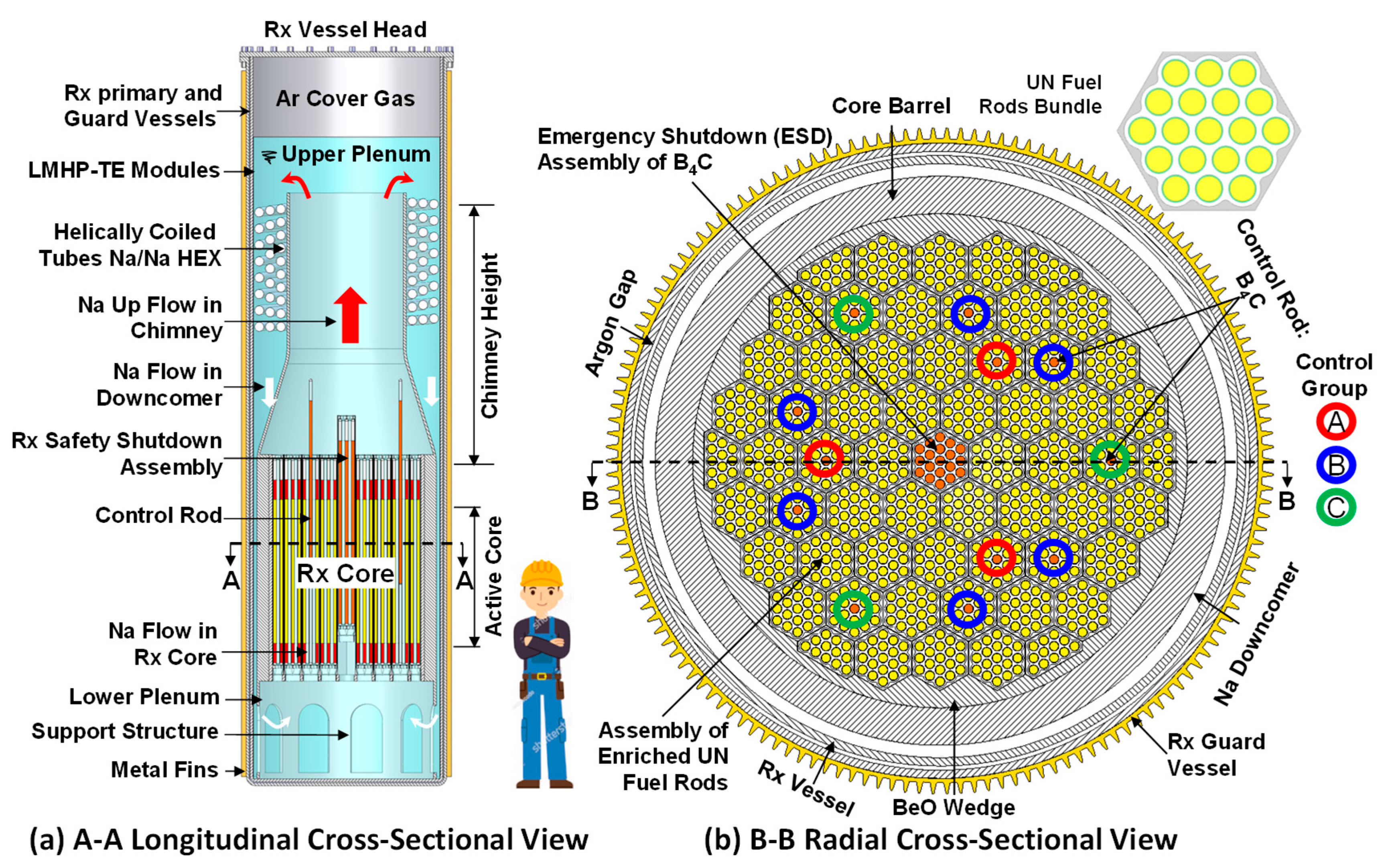
The present work trained the SL-LSTM and SAC-FNN algorithms using data sets generated by a developed MATLAB-Simulink transient model, or a digital twin, of the VSLLIM microreactor. This data is for simulated startup transients to steady power levels of 1.0–10 MW_th. The fast spectrum walk-away safe VSLLIM MMR design (Figure 1 and Figure 2) is cooled by natural circulation of in-vessel liquid sodium (Na) during nominal operation and after shutdown aided by a 2-m tall chimney and a helically coiled-tube Na/Na heat exchanger (HEX) placed at the top entrance to the downcomer (Figure 1 and Figure 2) [22,23].

It offers redundant control and passive removal of decay heat after shutdown and employes liquid metal heat-pipe thermoelectric (LMHP-TE) conversion modules cooled by natural convection of ambient air. They generate auxiliary DC power 24/7 during reactor operation and after shutdown, and in case of unlikely loss of both off-site and on-site power sources. This factory fabricated, assembled, and sealed modular microreactor can continuously generate 1.0 MW of thermal power for 92 full power years and up to 10.0 MW for ~5.9 Years (FPY), without refueling [22]. It arrives at the operating site on an 18-wheeler truck, by rail, or on a barge and is mounted underground on seismic isolation bearings to protect against earthquakes and an airplane crash or a missile impact (Figure 2).

Owing to the low vapor pressure of liquid sodium, the VSLLIM microreactor operates below atmospheric pressure, which eliminates the need for a pressure vessel. The primary and guard containments for the VSLLIM microreactor are separated by a small gap filled with argon gas, which houses sodium leak detectors. The low thermal conductivity argon gas decreases side heat losses during reactor operation. In the event of a loss of heat removal, due to a failure or malfunction of the in-vessel Na/Na HEX, the argon gas in the gap between the primary and guard vessels is replaced with liquid sodium. This facilitates the decay heat removal by in-vessel natural circulation of liquid sodium and by natural circulation of ambient air along the outer surface of the guard vessel (Figure 2) [26].

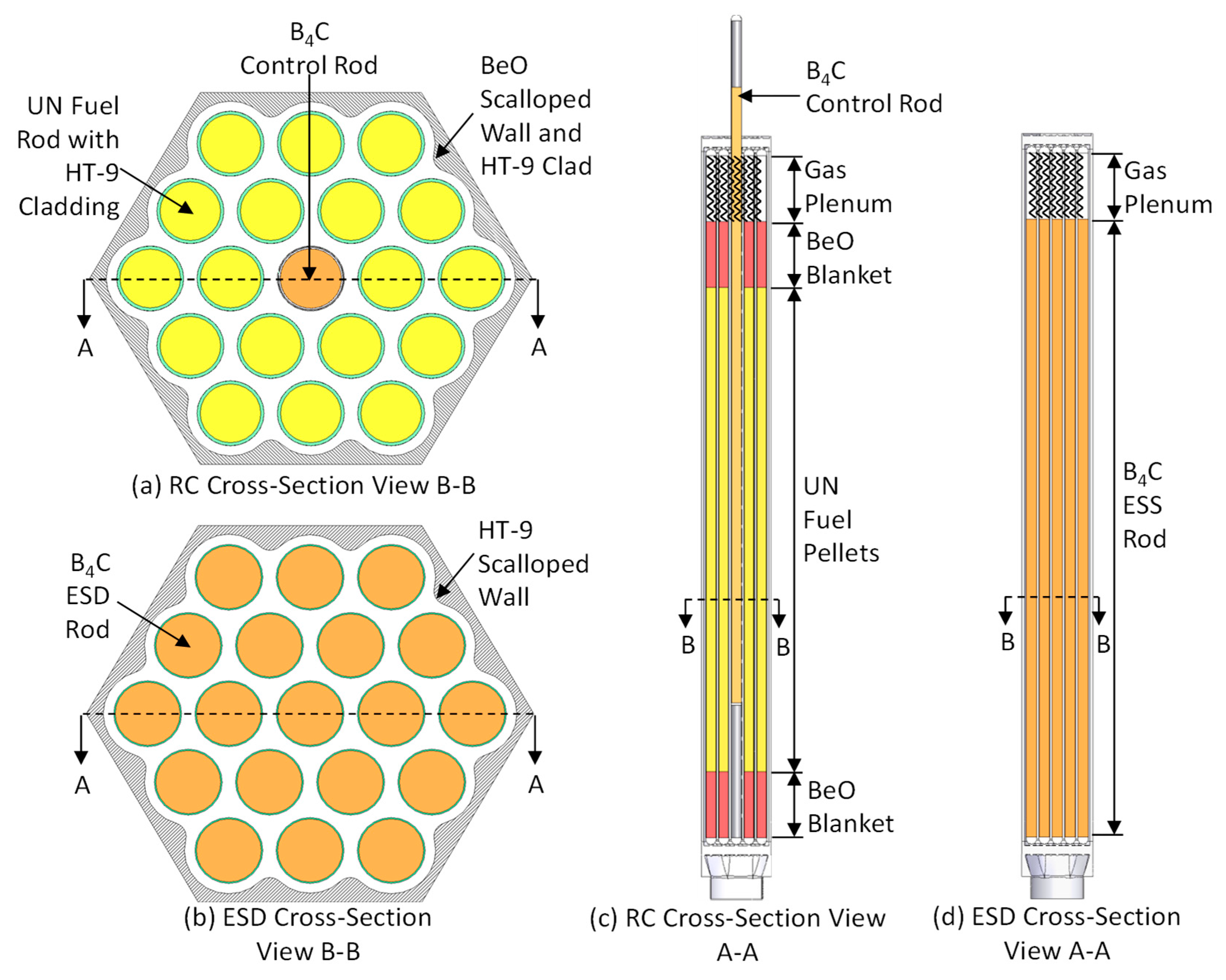
The VSLLIM microreactor core (Figure 1b) is loaded with hexagonal assemblies of 13.76 wt.% enriched UN fuel rods with HT-9 steel cladding and with scalloped BeO walls (Figure 3). The scalloped walls ensure that the liquid sodium flow is laterally uniform for cooling the fuel rods within the reactor core assemblies [22]. The fifty-four full hexagonal assemblies and the six partial assemblies of UN fuel rods in the reactor core are arranged in four concentric rings (Figure 1b). The full assemblies are loaded with 19 UN fuel rods, in a triangular lattice, and the partial corner assemblies contain 12 UN fuel rods each. The BeO wedges that surround the UN fuel assemblies in the core within the HT-9 steel core barrel serve as a radial neutron reflector (Figure 1b).

The VSLLIM microreactor has two independent and redundant means for the reactor control. The twelve B₄C Reactor Control (RC) rods located at the center of selected UN fuel assemblies in the second and third rings of the core (Figure 1b and Figure 3a,c) are for reactor control during operation and shutdown. These control rods fall into three groups, labeled A, B, and C, with separate drive motors (Figure 1b). Group A comprises three B₄C rods located at the center of fuel assemblies in the second ring of the reactor core. Group B comprises six B₄C rods in the fuel assemblies in the third ring of the core, and Group C comprises three B₄C rods in the fuel assemblies in the third ring of the core (Figure 1b).

The central Emergency Shut Down (ESD) assembly of 19 B₄C rods, 80% enriched in ¹⁰B, within scalloped HT-9 steel wall (Figure 1 and Figure 3b,d) provides independent shutdown of the reactor in case of an emergency. The next section briefly describes the VSLLIM microreactor digital twin dynamic model developed using the MATLAB Simulink platform [24]. This model generates the operation data sets for training and testing the trained SL-LSTM and SAC-FNN algorithms. They are implemented into the PLC controller of the VSLLIM microreactor during simulated startup and operation transients.

3. VSLLIM Digital Twin Model and Controller

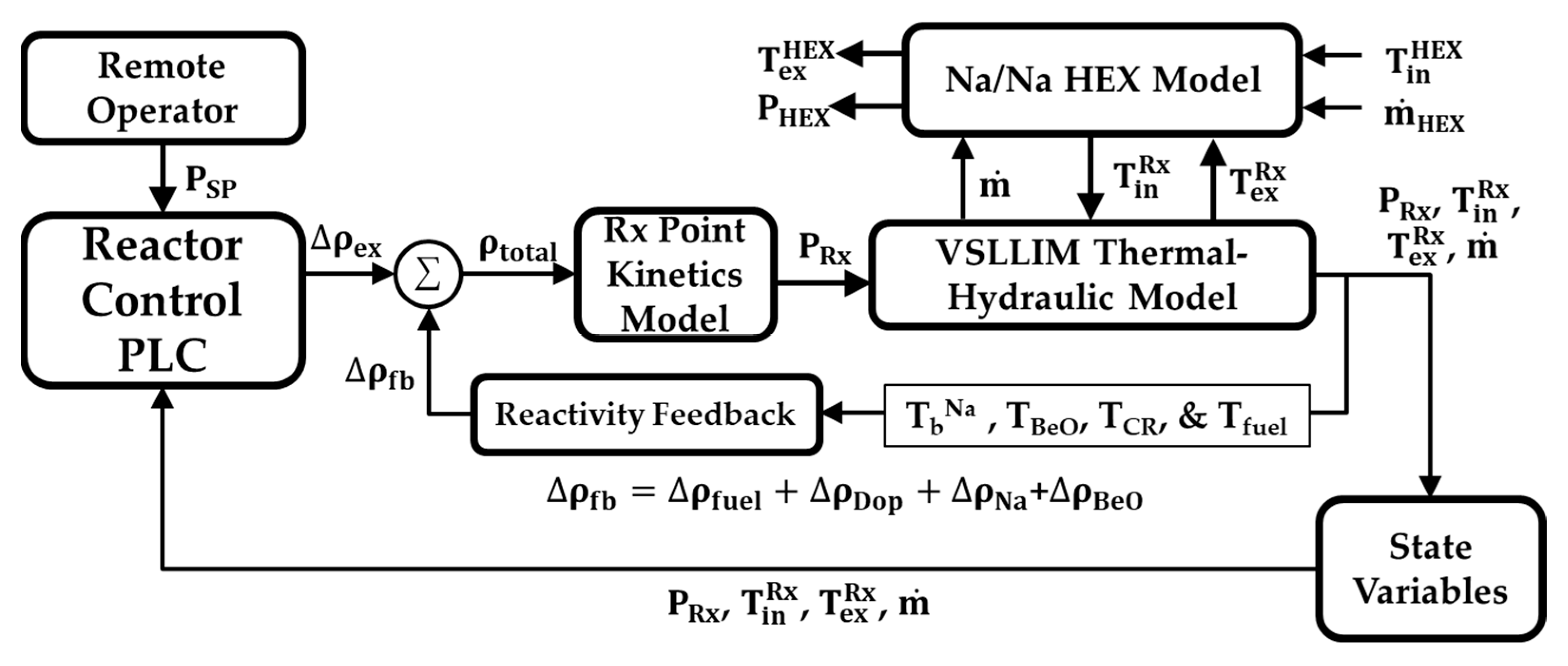
The VSLLIM digital twin dynamic model couples a six-group point kinetics sub-model [26] that accounts for the temperature reactivity feedback to thermal-hydraulics sub-models of the VSLLIM microreactor and the in-vessel Na/Na HEX (Figure 1a and Figure 4). The digital twin model uses the versatile MATLAB Simulink platform [24] to solve the governing equations in the coupled sub-models. The determined values of the physics-based operation parameters during the simulated startup transients are used for training the ML algorithms. These parameters are the reactor thermal power; the average temperatures of the UN fuel, HT-9 steel cladding, and structure and the circulating in-vessel liquid sodium in the reactor core; the mass flow rate and the temperature of the liquid sodium exiting the reactor core; and the temperatures of the rising sodium in the chimney, in the upper and lower plenums and on the shell side of the in-vessel Na/Na heat exchanger (Figure 1, Figure 2 and Figure 3). The Na/Na HEX maintains the temperature of the in-vessel liquid sodium entering the core at 610 K while the exit temperature that varies with the reactor thermal power is <800 K. At these temperatures, liquid sodium is compatible with the HT-9 steel cladding of the UN fuel rods and core structure [27]. The VSLLIM digital twin model uses the ode23s modified Rosenbrock solver in the MATLAB-Simulink platform to numerically solve the coupled point-kinetics sub-model to the overall energy and momentum balance equations of the reactor (Figure 4) with 20 ms time step size during the simulated transients.

The six-group point-kinetics sub-model calculates the transient changes in the reactor fission power, P_Rx, as a function of the external reactivity insertion, Δρ_ex, and the temperature reactivity feedback, Δρ_fb. The simulated startup transient of the VSLLIM microreactor begins after fully withdrawing the ESD central assembly. The inserted external reactivity is due to partially withdrawing the Groups A, B, and C control rods in the core. The temperature reactivity feedback, due to the decreases in the densities of the fuel, cladding, and liquid sodium in the reactor core and the Doppler broadening of the neutron cross sections in the UN fuel, are highly negative. However, the temperature reactivity feedback of the BeO in the radial and axial reflectors and in the scalloped walls of the UN fuel assemblies is slightly positive [22]. In the simulated startup transients, the total reactivity, ρ_total, in the VSLLIM microreactor core is the sum of the inserted external reactivity and the total temperature reactivity feedback (Figure 4).

The thermal-hydraulic sub-model of the reactor simultaneously solves the coupled energy balance equations in the UN fuel rods, core structure, and the in-vessel sodium and the momentum balance equation for natural circulation of the in-vessel liquid sodium coolant in the reactor core, chimney, and the downcomer. The sub-model of the Na/Na HEX (Figure 4) simultaneously solves the energy and momentum balance equations of the secondary liquid Na flowing inside the helically coiled tubes of the Na/Na heat exchanger and the in-vessel liquid sodium flow on the shell side of the HEX [22].

3.1. The VSLLIM Reactor Controllers

During simulated startup transients, the Reactor Control PLC commands the VSLLIM digital twin (Figure 4) and determines the rates and the magnitudes of the axial displacements of the ESD assembly and Groups A, B, and C control rods in the reactor core (Figure 1, Figure 2 and Figure 3). The PLC receives commands from the remote operator to start up or shut down the VSLLIM microreactor as well as specify the desired reactor power setpoint, P_SP (Figure 4). The digital twin model calculates the magnitude and the rate of the external reactivity insertion, Δρ_ex, in the reactor core as a function of the axial displacements of the control rods in the reactor core and passes it to the point-kinetics sub-model (Figure 4). The controller continues to adjust the axial displacement of the control rods until reaching the operator specified setpoint, P_SP, of the reactor thermal power.

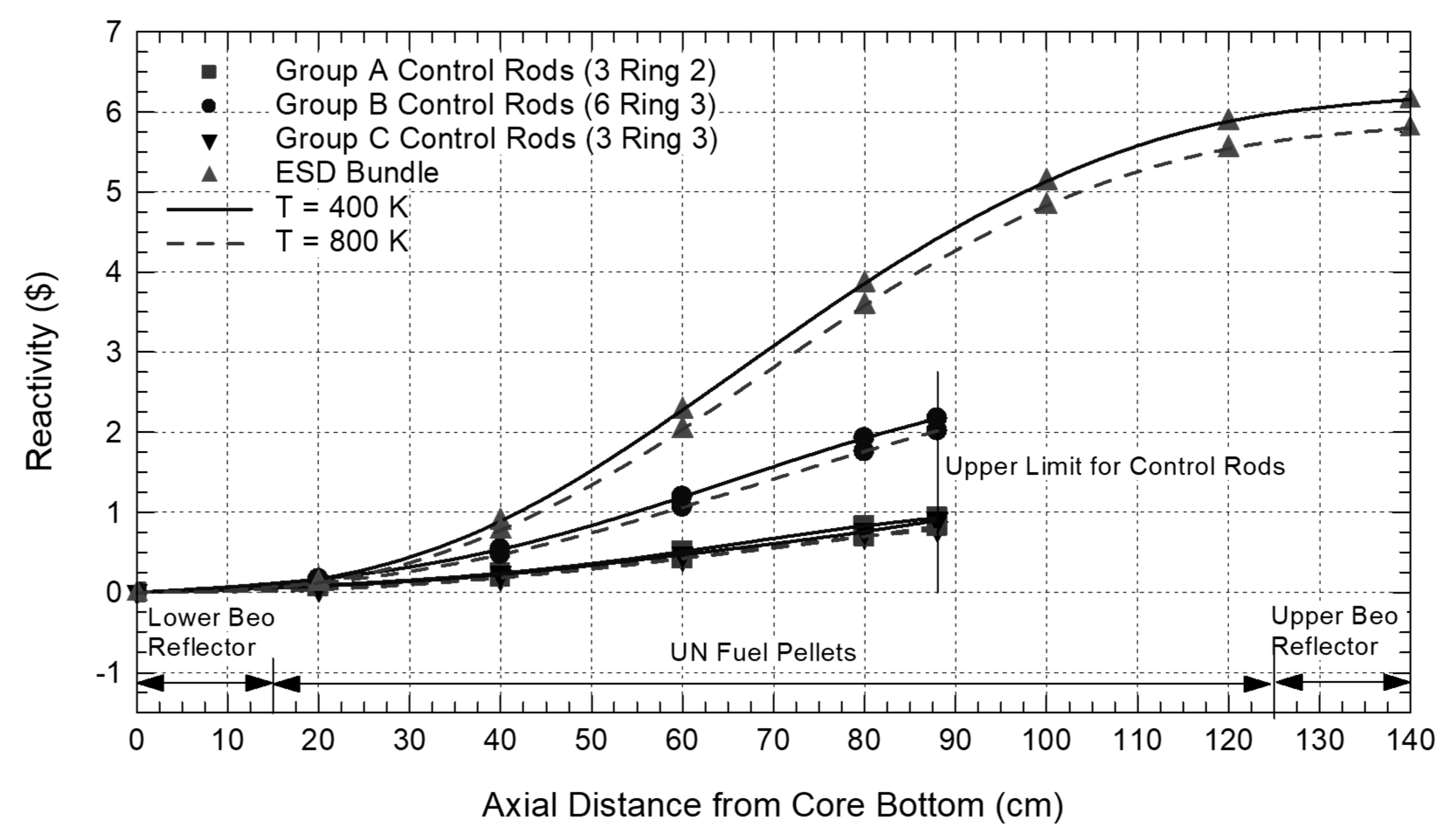
The results in Figure 5 are those of the performed neutronics analyses using the MCNP6 code [28] to determine the reactivity worth of each of the control rod groups in the VSLLIM reactor core as a function of axial displacement from the bottom of the core and the calculated mean temperatures in the core (Figure 5). This figure plots the calculated reactivity worth of the control rods in Groups A, B, and C and of the center ESD assembly as functions of axial displacement at isothermal temperatures of 400 K and 800 K. The vertical line in the figure marks the limit set for the axial withdrawal of the B₄C control rods in the core, which corresponds to 2/3 the active core height to speed up reactor shutdown in case of an emergency. The results assume that the control rods are in thermal equilibrium with the in-vessel liquid sodium in the reactor core.

3.1.1. Reactor Control PLC

Two Reactor Control PLC programs are developed to determine the control element positions, using (a) a modified Proportional–Differential (PD) controller and (b) an ML controller using the trained neural networks. The Reactor Control PLC program runs with a scan cycle time of 50 ms. It is sufficiently small to capture the response of the PLC to changes in the reactor operation. At the start of each scan cycle, the PLC reads the Modbus input registers holding the calculated values of the VSLLIM reactor state variables by the digital twin and the commands received from the remote human operator. The state variables include the reactor thermal power, the in-vessel and HEX Na flow rates, the core Na inlet and exit temperatures, the HEX Na inlet and exit temperatures, the calculated core reactivity, and the axial positions of the control rod groups and the ESD assembly. The PLC then acts on the received commands from the remote operator to determine the displacement rates for the control elements. At the end of the scan cycle the actions to move the control elements are written to the PLC’s Modbus output holding registers and communicated to the digital twin model of the VSLLIM microreactor.

During the simulated startup transients, the Reactor Control PLC brings the digital twin from an initial cold subcritical condition at a mean core temperature of 500 K to a steady full power operation at the reactor power setpoint specified by the remote operator. The PLC adjusts the axial displacement of the control rods to bring the reactor power to the setpoint specified by the remote operator, P_SP.

The Reactor Control PLC with the modified PD controller adjusts the rate of the axial displacement of the Group A and C control rods by a rate determined by the PD function depending on the input value of (P_SP − P_Rx). The displacement rate is limited to ≤0.125 mm/s to ensure a smooth increase in the thermal power reactor during the simulated startup transients. The modified PD controller uses a criterion derived from that proposed by Bernard, Lanning, and Ray [29] to adjust the axial withdrawal of the control rods to ensure smooth and gradual increase in the total reactivity, ρ_total, and hence in the reactor power and temperatures, during the startup transient. This criterion is given as follows:

$${\rho }_{total}<{\displaystyle \frac{1}{\alpha }}\left[{\displaystyle \frac{\left|\frac{d\rho }{dt}\right|}{{\lambda }_e}}+\left|{\displaystyle \frac{d\rho }{dt}}\right|\tau \mathit{ln}{\displaystyle \frac{P_{SP}}{P_{Rx}}}\right],$$

(1)

In this expression, α is a scaling coefficient, ${\displaystyle \frac{d\rho }{dt}}$ is the rate of change in the total reactivity, τ is the reactor period, and λ_e is the effective decay constant for the six delayed neutron groups in the reactor’s point-kinetics sub-model. The scaling coefficient provides adequate time for the total reactivity to account for the delayed negative temperature reactivity feedback due to the thermal inertia of the system before further displacing the control rods. A value of α = 25 is used in the present work, for a good balance between shortening the startup time and ensuring smooth increases in the reactor thermal power and the core temperatures during the simulated startup transients.

The Reactor Control PLC program incorporating the ML SL-LSTM and SAC-FNN algorithms inputs the current state variables to the trained neural network and determines the position of the reactor control elements from the network’s output. The displacement rate of the Group A and C control rods is determined from the difference between the desired control rods’ displacement and the present axial displacement, divided by the step period of 0.4 s. The obtained displacement rate is limited to ≤0.125 mm/s, same as in the PLC with PD controller. Unlike the PLC with PD controller, the PLC program with the ML algorithms does not explicitly limit the control rod displacement using the restriction criteria in Equation (1). Instead, the PLC relies on the trained ML algorithm to adjust the control rod positions and ensure a smooth increase or decrease in the reactor power.

3.1.2. HEX Secondary Flow PLC

In addition to the Reactor Control PLC, the VSLLIM microreactor has a PLC that adjusts the secondary Na flow through the helically coiled tubes of the Na/Na HEX using a Proportional–Integral (PI) control function (Figure 1). This function maintains the temperature of the in-vessel liquid Na entering the reactor core, T_in, constant at ~610 K. The input to the HEX PLC PI controller is the difference between the current in-vessel Na inlet temperature to the reactor core, T_in, and the setpoint of 610 K.

3.2. A Simulated Startup Transient of VSLLIM Microreactor

The VSLLIM microreactor digital twin model (Figure 4) simulates reactor startup from an initial subcritical condition to steady state operation at a user specified reactor thermal power setpoint. Figure 6 presents the results of a simulated startup transient based on the control rods’ reactivity worths in Figure 5. The startup transient in Figure 6 begins with the reactor initially subcritical with the in-vessel liquid sodium and the reactor core at 500 K. The startup procedures begin with the Reactor Control PLC fully withdrawing the ESD center assembly from the reactor core over a period of 240 s (Point 1 in Figure 6a). At such point, the reactor is still subcritical. Then the Reactor Control PLC axially withdraws the Group B control rods by 0.77 m over a period of 180 s for the reactor to achieve criticality (Point 2 in Figure 6a). Next, the PLC simultaneously withdraws the Group A and C control rods in the reactor core at a constant rate of 0.75 mm/s until the reactor power reaches a steady value of 100 kW_th (Point 3 in Figure 6a,b). Subsequently, the PD controller manages the withdrawal of the control rods to increase the reactor power to setpoint P_SP,1 = 0.5 MW_th. The PLC limits the movement rate of the Group A and C control rods to ≤0.125 mm/s to ensure a smooth rise of both the reactor power and the exit temperature of the liquid Na in core (Figure 6b,c). The PLC for the Na/Na HEX increases the flow rate of the secondary liquid sodium in the helically coiled tubes to maintain the inlet temperature of the in-vessel sodium into the reactor core, T_in, at 610 K (Figure 6c,d). The reactor reaches steady state power of 0.5 MW_th at t = 2.38 h into the startup sequence (Figure 6b).

The VSLLIM reactor operates at the power setpoint of 0.5 MW_th for a period allowing the remote operator and the on-site diagnostics to check out the systems prior to resuming the increase in the reactor power to 10 MW_th. The remote operator sends a command to the reactor controller to increase the reactor thermal power setpoint from 0.5 MW_th to 10 MW_th (Point 6 in Figure 6). The PD controller simultaneously displaces the Group A and C control rods to increase the external reactivity insertion and hence the reactor thermal power (Figure 6a,b), the circulation rate of the in-vessel liquid sodium, and the sodium exit temperature from the reactor core. The values of these parameters increase steadily over a period of 4.75 h until the reactor power reaches and levels off at 10 MW_th (Point 7 in Figure 6). The corresponding temperature and circulation rate of the in-vessel liquid sodium at the reactor core exit are 780.6 K, and 46.0 kg/s, respectively.

3.3. Machine-Learning Training Data

The VSLLIM microreactor digital twin (Figure 4) generates the target data sets used to train the SL-LSTM and SAC-FNN algorithms. 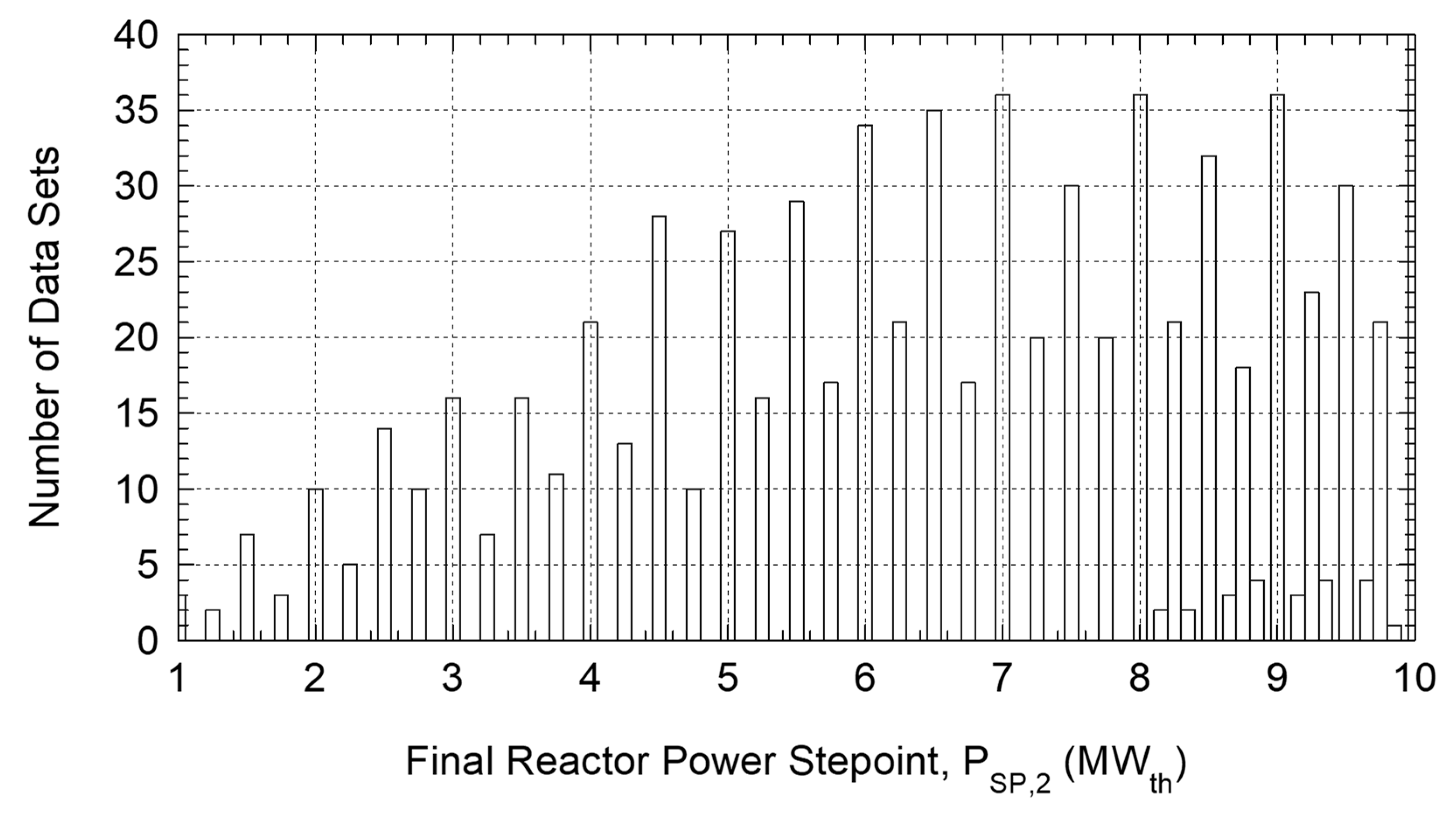In the simulated startup transients, the Reactor Control PLC with PD controller manages the displacement of the Group A and C control rods in the core to increase the reactor thermal power in increments of 0.25 MW_th until reaching the low power setpoints P_SP,1 = 0.5–9.75 MW_th, and then the high setpoints P_SP,2 = 1.0–10.0 MW_th. The data sets in Figure 7 are those generated for different periods of 200 to 367 min during the simulated startup transients to change the reactor power from P_SP,1 to P_SP,2. Generating the data sets with the physics-based VSLLIM digital twin model ensures that the operation state variables used as features and targets are physically coupled as in the real reactor and are not independently varied. The VSLLIM digital twin model generated a total of 797 data sets comprising more than 956 million data points covering the VSLLIM microreactor power ranging from 0.5 to10 MW_th (Figure 7). The SL-LSTM algorithm used the data sets for training, validation, and testing, while the SAC-FNN algorithm used the generated data as a target.

4. Training the SL-LSTM Algorithm

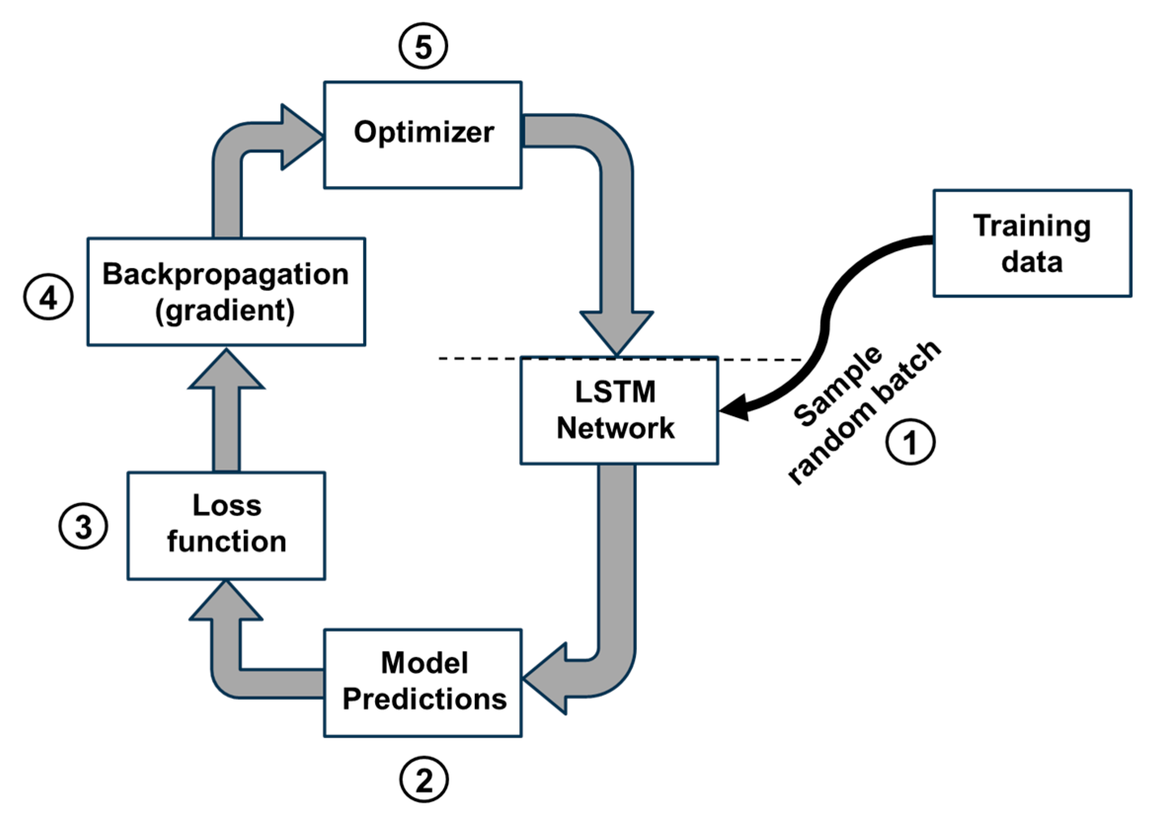
The training of the SL-LSTM algorithm used the values of the input parameters (referred to as features) and of the desired output (referred to as the target) and builds a function to predict output for unseen input data [4]. This algorithm uses LSTM recurrent neural networks [30] to process sequential time-series data inputs [31] and trains in iterative cycles referred to as epochs. Within each epoch the algorithm undergoes the five operations shown in Figure 8. First, it shuffles the order of the data sets provided and then randomly samples a mini batch of parameters (Point 1 in Figure 8). Shuffling the training data sets avoids learning biases associated with the order of the data within the sets.

The predictions generated by the LSTM network are based on the supplied input parameters in randomly selected mini batches from the training data sets (Point 2 in Figure 8). It then compares the predictions to the target values in the training data sets and calculates a loss function (Point 3 in Figure 8). Next, the algorithm performs backpropagation to calculate the gradients of the loss function with respect to the network’s parameters (Point 4 in Figure 8). These gradients are supplied to the optimizer module to update the weight and bias matrices of the LSTM network (Point 5 in Figure 8). These five steps are performed iteratively within each epoch for all the data in the training sets. The training process continues for sequential epochs until the value of the loss function converges and no longer changes with additional training epochs.

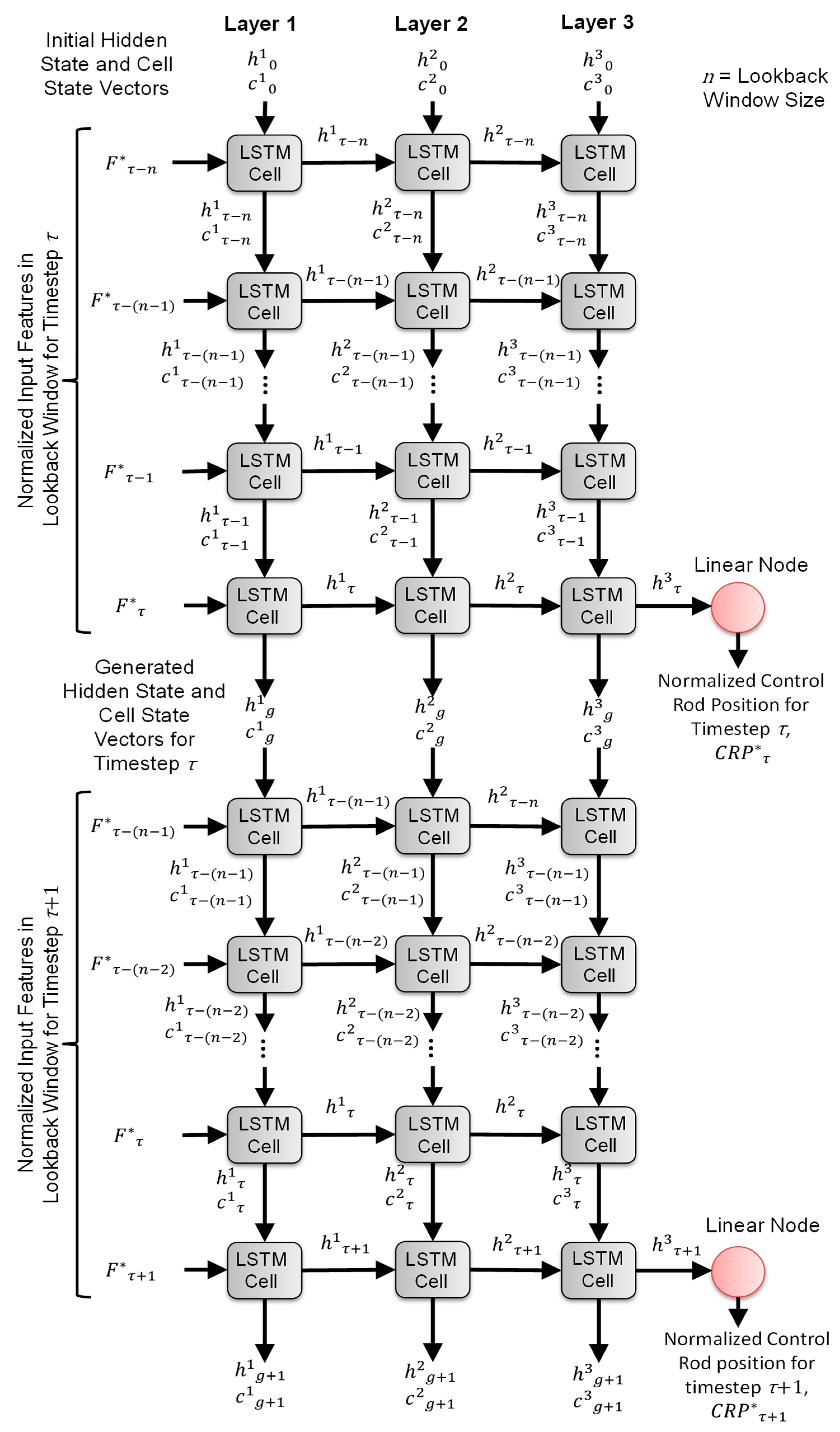
The python program that incorporates the SL-LSTM algorithm (Figure 9) uses the PyTorch 2.2 library [32]. Figure 9 is a flow diagram for two subsequent timesteps of the LSTM network in the present work, which has three layers of cells. The number of cells in each layer equals the size of the Lookback Window, n (Figure 9). In each timestep the Lookback Window includes the values of the features for the past (n) timesteps. For the LSTM network to learn the trends in the time-series data, the input features to a timestep (τ) includes the values for the timesteps (τ − n) to (τ) [30].

The trained SL-LSTM algorithm in the present work selects five primary features, namely: the reactor thermal power setpoint, and the transient values of the reactor thermal power, the reactor core inlet and exit temperatures, and the mass flow rate of the circulating liquid sodium through the core. Each data set contains the transient values of these parameters with a temporal discretization of 0.2 s. The LSTM network estimates a single target value of the normalized position of the Group A and C Control Rods, CRP*. PyTorch normalizes the values of the features to the first layer of cells (Figure 9) to the highest ($x_{max})$ and lowest $(x_{min}$) values in any of the supplied 797 training data sets. This ensures that the values of the normalized feature fall within the interval from 0 to 1. For each feature value, x, the normalized value, x*, is calculated as follows:

$$x^{\ast }={\displaystyle \frac{x- x_{min}}{x_{max}-x_{min}}}.$$

(2)

The features use the same values of x_max and x_min to train the SL-LSTM algorithm. The cells in the network receive and output data in two directions (Figure 9). For a given timestep (τ) the arrays of normalized features F* in the lookback window pass from the left in Figure 9 to the LSTM cells in the first layer. These cells also receive the hidden state, h, and the cell state, c, vectors passed from the top down. The algorithm randomly generates the initial values for the hidden state and cell state vectors, h_o and c_o. The values in the three layers in Figure 9 are numerated as h¹, h², and h³, and c¹, c², and c³, respectively.

The present values of the cells’ weight and bias matrices are used to compute the output vectors for the hidden states. The output hidden and cell state vectors pass downward to the cell within the same layer for the subsequent timestep in the lookback window (Figure 9). The hidden state vector also passes to the cell in the next layer for the same timestep in the lookback window (Figure 9).

The learned parameters within the cells control how it “remembers” or “forgets” information stored within the cell and to learn the time-dependent trends of the training data for calculating the output hidden state vectors. The hidden and state vectors pass along the network from left to right and from top to bottom. This is until the present timestep (τ) in the last layer (Layer 3 in Figure 9), where the cell calculates the output hidden state vector h_τ³. This vector passes to a linear node, which converts its output to a single scalar value between 0 and 1. This value is the predicted normalized position for the Group A and C control rods, CRP*.

The predicted axial displacement position, CRP, of the control rods is determined from de-normalizing the output value from the linear node by reversing the min–max normalizing in PyTorch as follows:

$$x= x^{\ast }\left(x_{max}-x_{min}\right)+x_{min},$$

(3)

The generated hidden and state vectors for the LSTM cells at the present timestep (τ) in the lookback window, h_g and c_g, are treated as the initial states to cells when calculating the CRP* for the next timestep (τ + 1) (Figure 9). The lookback window for this timestep shifts forward in time by one timestep and includes the input features for the timesteps (τ + 1) to (τ − (n − 1)).

The 797 data sets generated by the VSLLIM digital twin model (Figure 4) are divided into three groups, for training, validation, and testing. The SL-LSTM algorithm uses the Root Mean Square Error (RMSE) for training, testing, and validation loss function. This is calculated based on the difference between the predicted positions of the control rods, x, and the “true” values in the training datasets, as

$$RMSE=\sqrt{ {\displaystyle \frac{1}{N}}{{\displaystyle \sum }}_{i=1}^N{\left(x-x_{target}\right)}^2},$$

(4)

In this expression, N is the total number of training data sets. The accuracy of the predictions is the percent relative error of the predicted position of the control rods from the target values in the data sets, expressed as

$$Accuracy\left(\%\right)=100\times {\displaystyle \frac{\left(x-x_{target}\right)}{x_{target}}},$$

(5)

The SL-LSTM algorithm also employs the AdamW optimizer with a constant weight decay = 0.1. During training, the algorithm updates the weights and biases for the LSTM cells based on the calculated value of the loss function.

During the validation phase, the SL-LSTM algorithm calculates the RMSE of the predicted position of the control rod position relative to the values in the validation datasets, called the validation loss, but does not update the weights and biases of the LSTM cells. The training loss determines how well the predictions of a trained model fit the provided data sets for training, while the validation loss indicates the expected performance for data not included in the training sets. The validation uses independent data sets to avoid underfitting and overfitting. The testing data sets are used to quantify the testing loss and accuracy of the trained SL-LSTM algorithm for predicting the displacements of the control rods in the VSLLIM reactor core, compared to those of the PLC with PD controller.

Results of the Trained SL-LSTM Algorithms

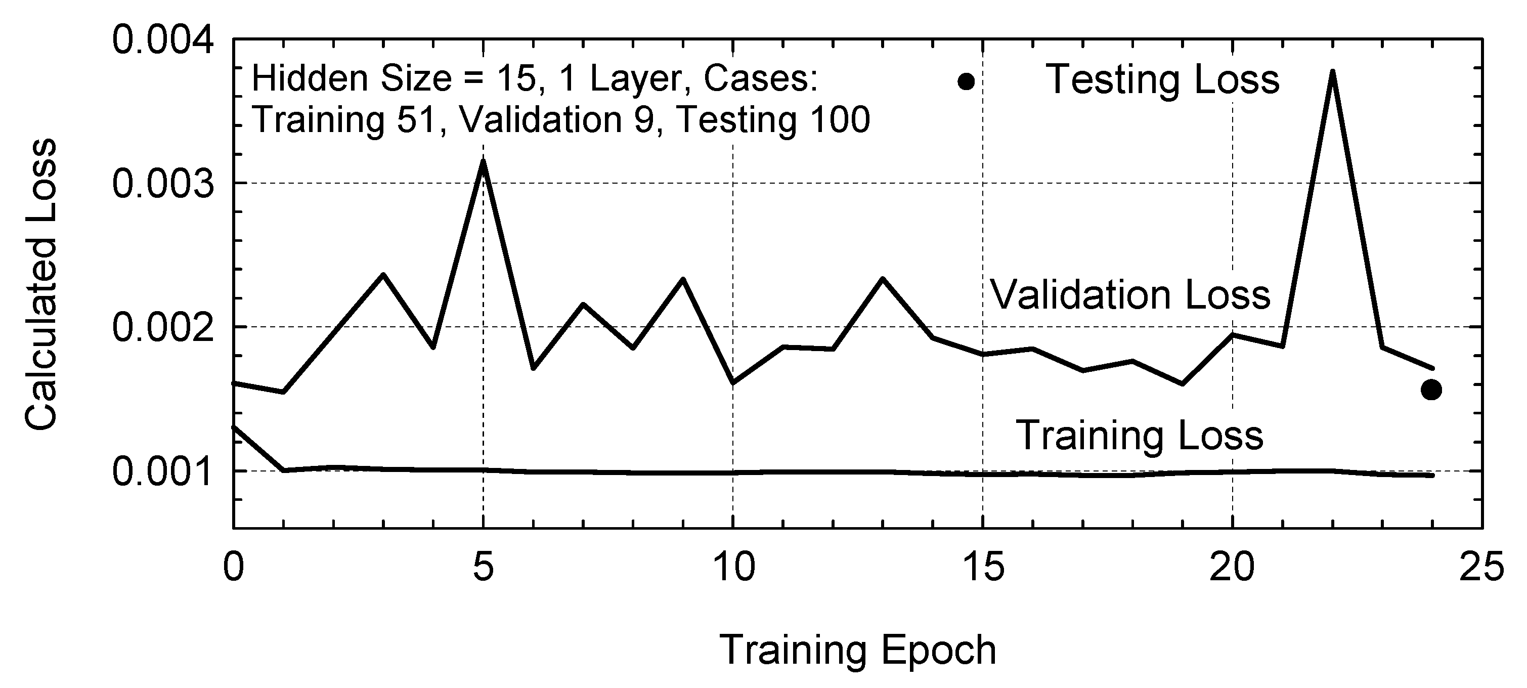
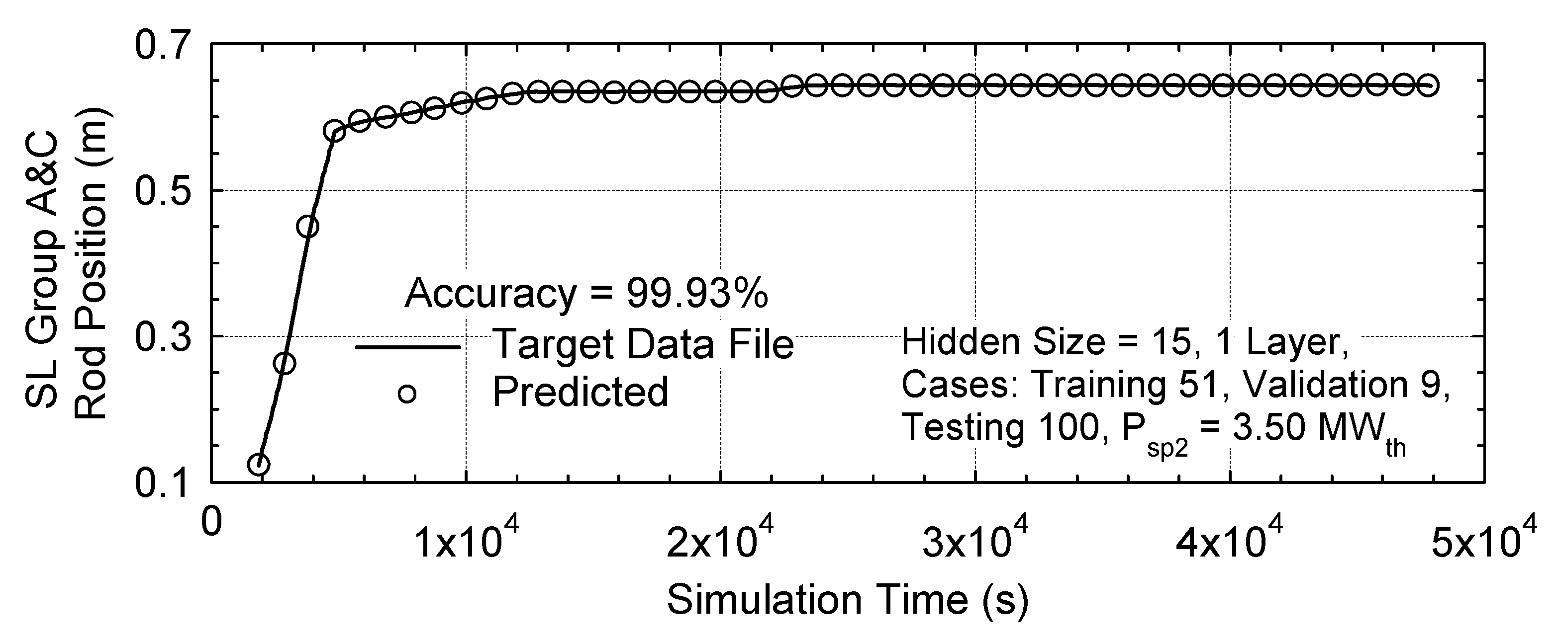
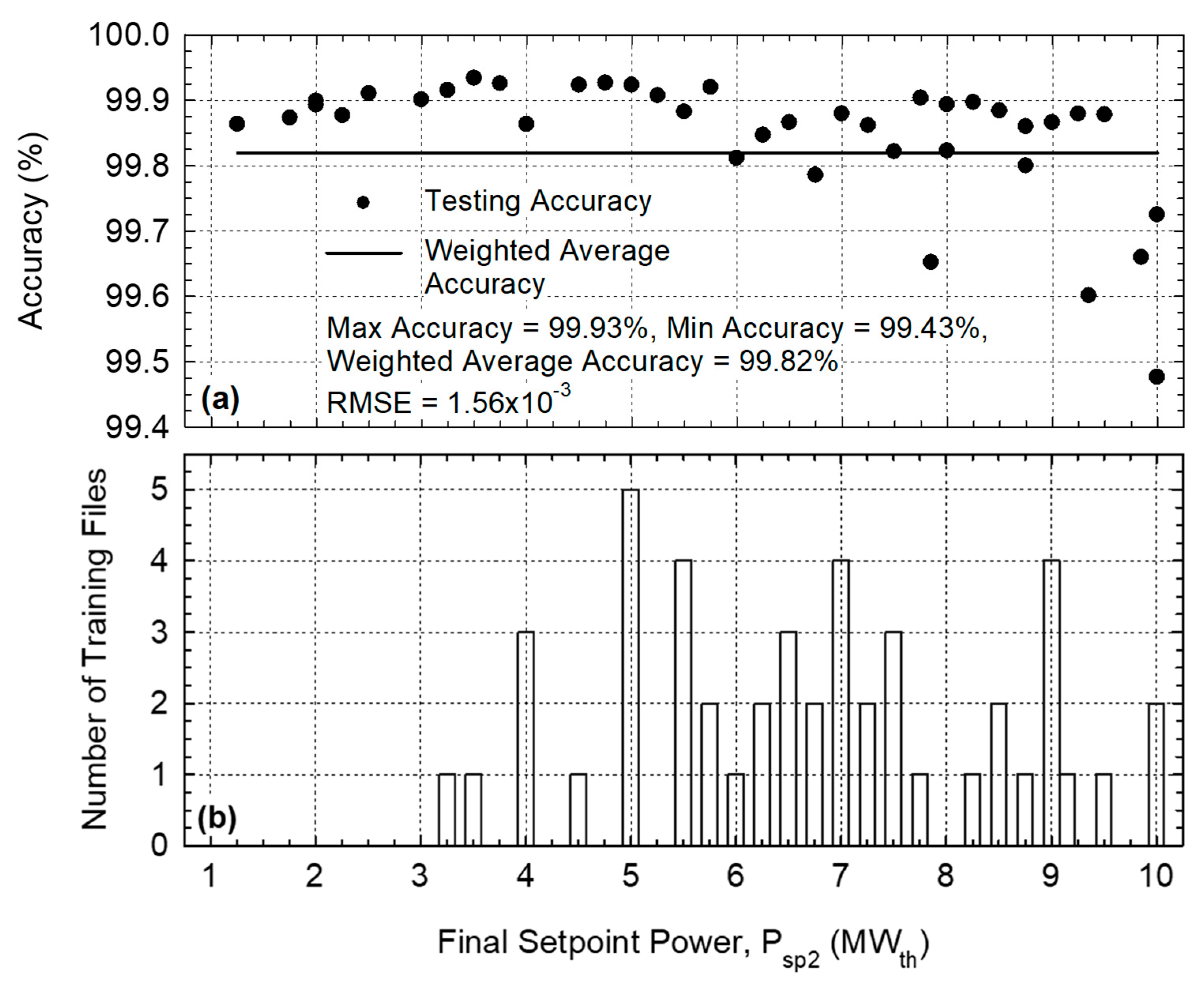
The performed parametric analyses optimize the hyperparameters of the trained SL-LSTM algorithm and investigate the effect of different parameters on accuracy and applicability to the controller of the VSLLIM microreactor. Appendix A details the investigated ranges and the effects of the hyperparameters on the accuracy of the trained SL-LSTM algorithm. Figure 10, Figure 11 and Figure 12 present example test results for a trained SL-LSTM algorithm with one layer of neurons, a hidden size of 15, and a learning rate of 0.001, using fifty-one randomly selected training data sets, nine validation sets, and one hundred testing sets. Figure 10 compares the calculated RMSE curves for training and validation losses. The training loss decreases to ~1 × 10⁻³ after only three epochs, and changes slightly thereafter (Figure 10). The validation loss oscillates but is of the same magnitude as the training loss (~3 × 10⁻³). These results confirm the successful training of the SL-LSTM algorithm after only a few epochs. The low testing loss of 1.56 × 10⁻³ confirms good predictive performance of the trained SL-LSTM algorithm for the 100 testing cases not included in its training data (Figure 10).

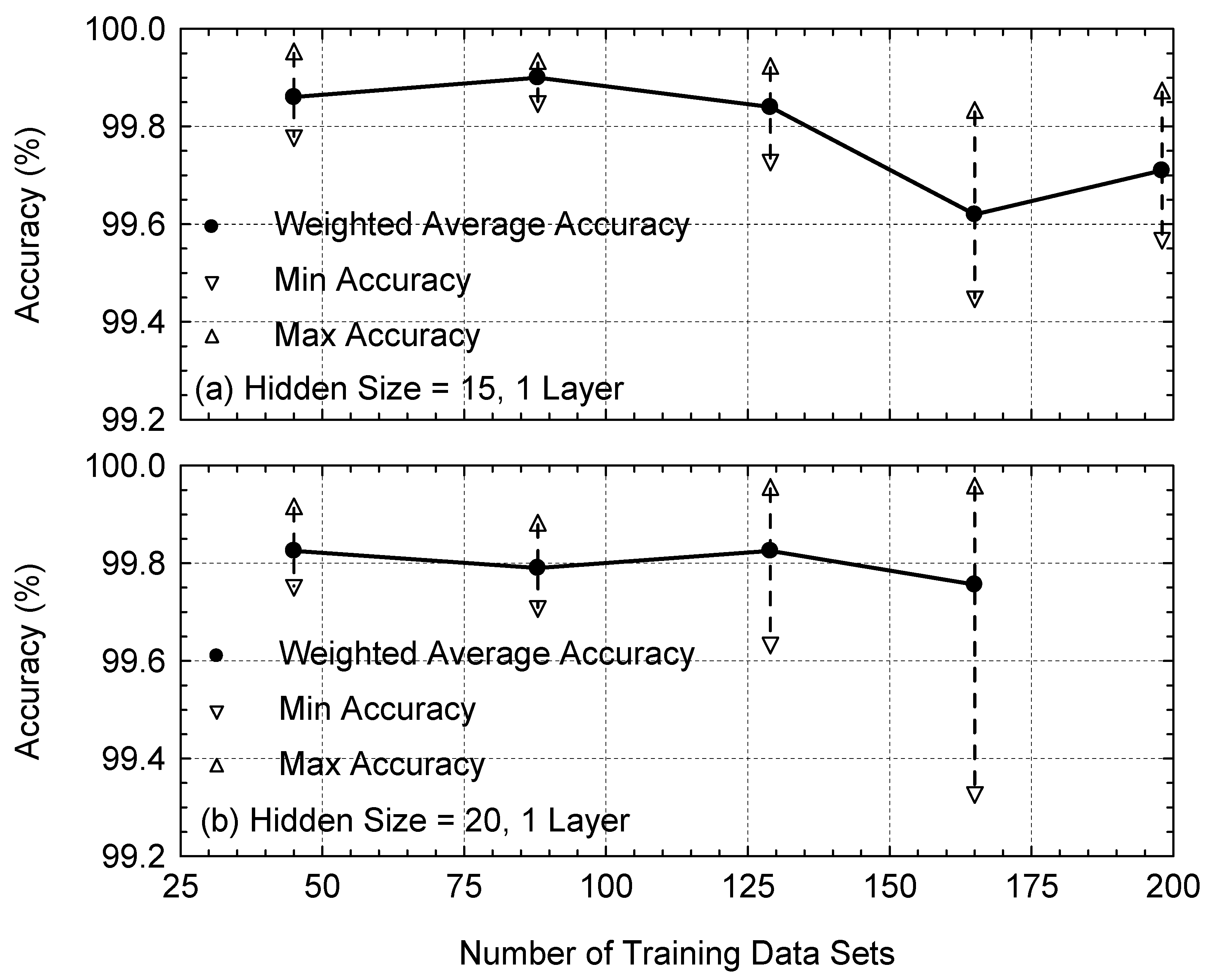
Figure 11 compares the predicted displacements of the Group A and C control rods in the VSLLIM reactor core in a testing case with a final power setpoint, P_sp,2, of 3.5 MW_th. The predictions of the trained SL-LSTM algorithms agree with an accuracy of 99.93%. Figure 12a,b show that the testing accuracies are similarly good for the other VSLLIM startup simulations. The determined accuracy displays a small spread between 99.43% and 99.93%, with an average weighted accuracy of 99.82% for the 100 testing data sets, with a testing loss of 1.56 × 10⁻³ (Figure 12a). These randomly selected testing data sets cover a range of final power setpoints from 3 to 10 MW_th (Figure 12b).

5. Training the SAC-FNN Algorithm

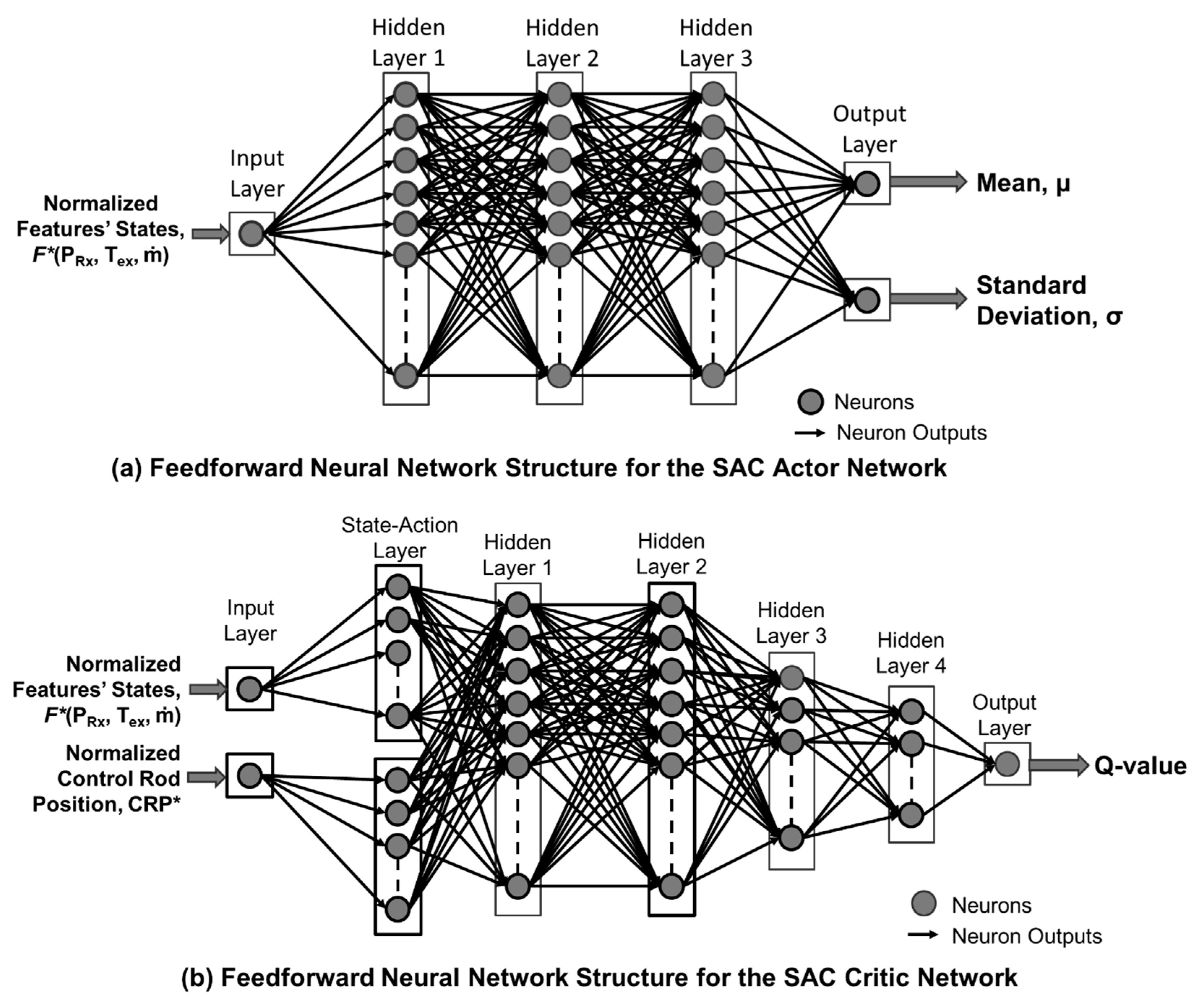
The FNN in the algorithm processes information in one direction, where the output values for a layer of neurons pass on to the inputs of the next layer of neurons (Figure 13). Unlike the SL-LSTM algorithm, the SAC-FNN algorithm does not make predictions based on previous timesteps’ data. Instead, the output is solely based on the present values of the features, F (Figure 13a,b). The Actor Network comprises an input layer with a single neuron, three hidden layers of many neurons each, and an output layer with two neurons (Figure 13a). The features are normalized using the same min–max normalization function used for the SL-LSTM algorithm Equation (2).

The array of normalized features, F*, passes through the input layer (Figure 13a), which passes the output values to the neurons in the first hidden layer. The output values, Y, are calculated from input values, X, based on the values of the neurons’ weight, w, and bias, b, and an activation function α, as follows:

$$Y= \alpha \left(w X+b\right),$$

(6)

The SAC-FNN algorithm updates the learned weight and bias parameters of the neurons in the FNNs during the training process. The mean (μ) and standard deviation (σ) output by the Actor Network define a normal distribution of the normalized control rod displacements (Figure 13a). The two neurons in the input layer of the Critic Network are for the array of the normalized state values, F*, and the corresponding normalized control rods position CRP* (Figure 13b). These values pass through the neurons in the State-Action layer and sequentially to each of the four hidden layers for the Critic Network. The output layer calculates the approximate action function, referred to as the Q-value.

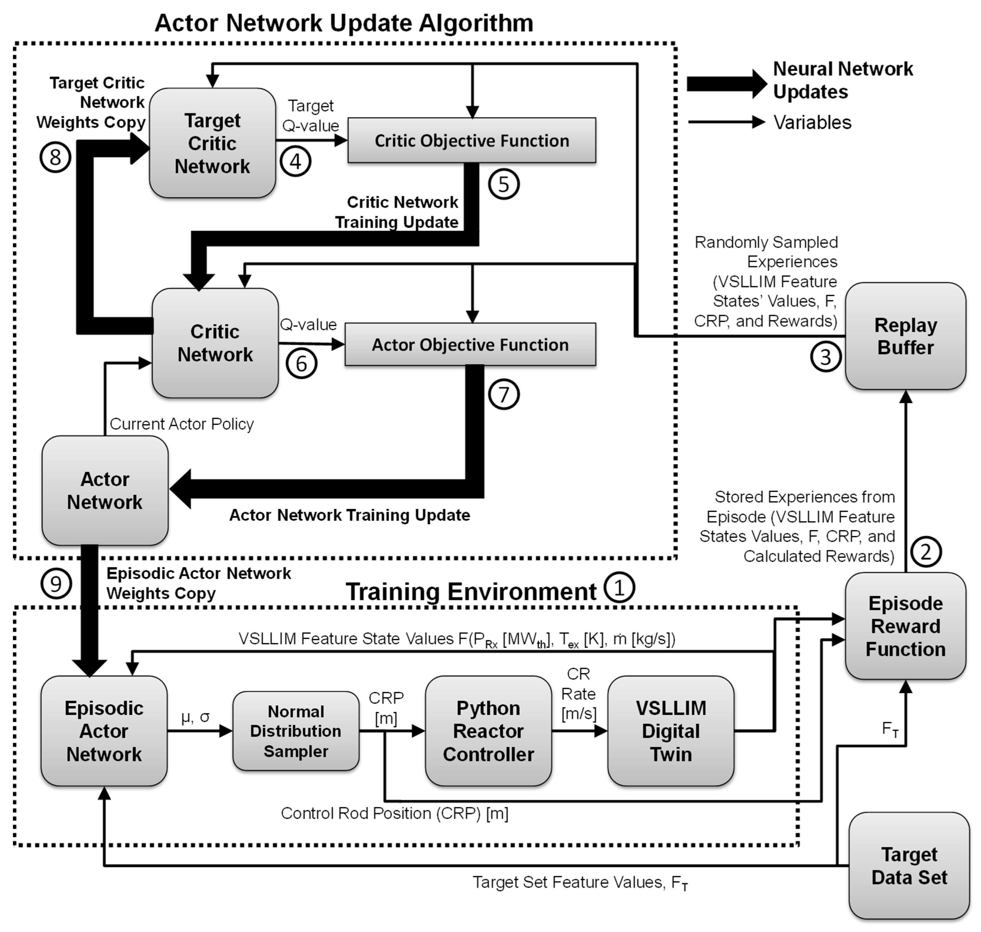
The SAC-FNN algorithm is incorporated into a Python program using Tensorflow [33] with the Keras ML libraries [34] based on those proposed by Bae, Kim, and Lee [21]. These include a Training Environment and an Actor Network Update Algorithm (Figure 14). The Training Environment (Point 1 in Figure 14) couples the Episodic Actor Network to the Python Reactor Controller (described in Section 3.1). The environment links the controller to the VSLLIM digital twin model to control the movement of the control rods during the performed transient startup scenario (Figure 6). During each training episode the controller attempts to follow the startup scenario in the user supplied Target Data Set and bring the VSLLIM microreactor to the specified target power setpoint, P_sp,2. The trained SAC-FNN algorithm learns to reproduce the startup control actions of the PD controller displayed in the Target Data sets (Figure 14). These sets are selected from among the 797 sets generated by the digital twin model of the VSLLIM microreactor (Figure 7).

In each timestep of the simulated startup transient (e.g., Figure 6), the Episodic Actor Network (Figure 13a) receives the features, F, from the VSLLIM digital twin model (Figure 4) and the mean and standard deviation of the output data. The Normal Distribution Sampler then samples a CRP* from the developed normal distribution of the calculated values of μ and σ. These values are de-normalized using the defined min–max de-normalization Equation (3) and are passed on to the Python Controller.

The controller calculates the displacement rates of the Group A and C control rods in the core of the VSLLIM microreactor (Figure 1). These rates are based on the difference between the predicted position of the control rods from the FNN and the present position in the digital twin model of the reactor. It then communicates the displacement rate of the control rods to the digital twin model to adjust the reactor operation parameters in the next simulation timestep. The Python Controller communicates with the digital twin using a POSIX shared memory function. The MATLAB engine for python [24] launches the digital twin model of the VSLLIM reactor at the start of each training episode (Figure 14).

At the end of the episode the reward value is calculated by the reward function for each timestep of the simulated transient (Point 2 in Figure 14). The reward function for the SAC-FNN algorithm uses a distance-based proportional reward Equation (7). A reward, R_i, is calculated separately for each of the three features, i, using the percent relative difference, E, between the value determined by the digital twin model of the microreactor and that in the target set, as follows:

$$R_i=10-\left(100\times \left|{\displaystyle \frac{x-x_{target}}{x_{target}}}\right|\right), for E<10\%$$

(7a)

$$R_i=-10, for E\ge 10\%$$

(7b)

The region in which E ≥ 10% defines the termination range. A reward of −10 is given for each time step in which the features are within that range. The episode is terminated if any of the three features stays in the termination range for a continuous period of more than 60 s. This period provides the reactor controller time to self-correct back into the desirable region of E < 10%. The episode’s total reward is the sum of the cumulative reward for each of the three features over all the timestep in the training episode. Therefore, episodes that terminate early receive a smaller total reward, while episodes where the controller maintains the features within the allowed range for a longer period will receive a higher total reward. The minimum total reward for an episode is limited to zero because negative rewards for training episodes resulted in poor learning for the Actor network.

The algorithm randomly selects sets of the features at different points of the episode, and the corresponding control rods position predicted, and the calculated rewards at the end of each episode. These values, referred to as experiences, are stored within the Replay Buffer (Point 3 in Figure 14). They are of the current and all previous training episodes. The SAC-FNN algorithm randomly samples a batch of experiences from the Replay Buffer and passes them to the Actor Network Update function to update the Actor Network to improve its performance. Updates to the networks occur only at the end of the episode, and the algorithm does not update the Actor Network while it is controlling the digital twin model. The update function comprises the Actor Network, the Critic Network, and the Target Critic Network (Figure 14).

The Actor Network learns a policy to determine the control actions, the Critic Network learns the action–value function (called the Q-value function) to update the policy of the Actor Network, and the Target Critic Network helps stabilize the Critic Network by evaluating its performance in updating the policy of the Actor Network. The Target Critic Network calculates a target Q-value (Point 4 in Figure 14) that passes on to the Critic Objective Function to estimate the expected future reward for the Actor Network. This value is compared to past reward values to determine the updates for the weight and bias matrices in Critic Network (Point 5 in Figure 14).

The updated Critic Network uses sampled experiences from the Replay Buffer and the policy actions of the Actor Network to calculate the Q-value for the Actor Objective Function (Point 6 in Figure 14). It then updates the weights and biases in the Actor Network to maximize the episodic reward (Point 7 in Figure 14). The SAC algorithm copies the parameters of the Critic Network to the Target Critic Network to improve the controller’s behavior in the next episode (Points 8, 9 in Figure 14). The process continues in subsequent episodes until the SAC algorithm successfully trains the Episodic Actor Network. A successful episode is the one in which the Episodic Actor Network of the trained SAC-FNN algorithm successfully increases the thermal power of the VSLLIM microreactor during the simulated startup transient from an initial setpoint P_sp,1 = 0.5 MW_th, to the final setpoint P_sp,2 = 10.0 MW_th.

Implemented SAC-FNN Algorithm Results

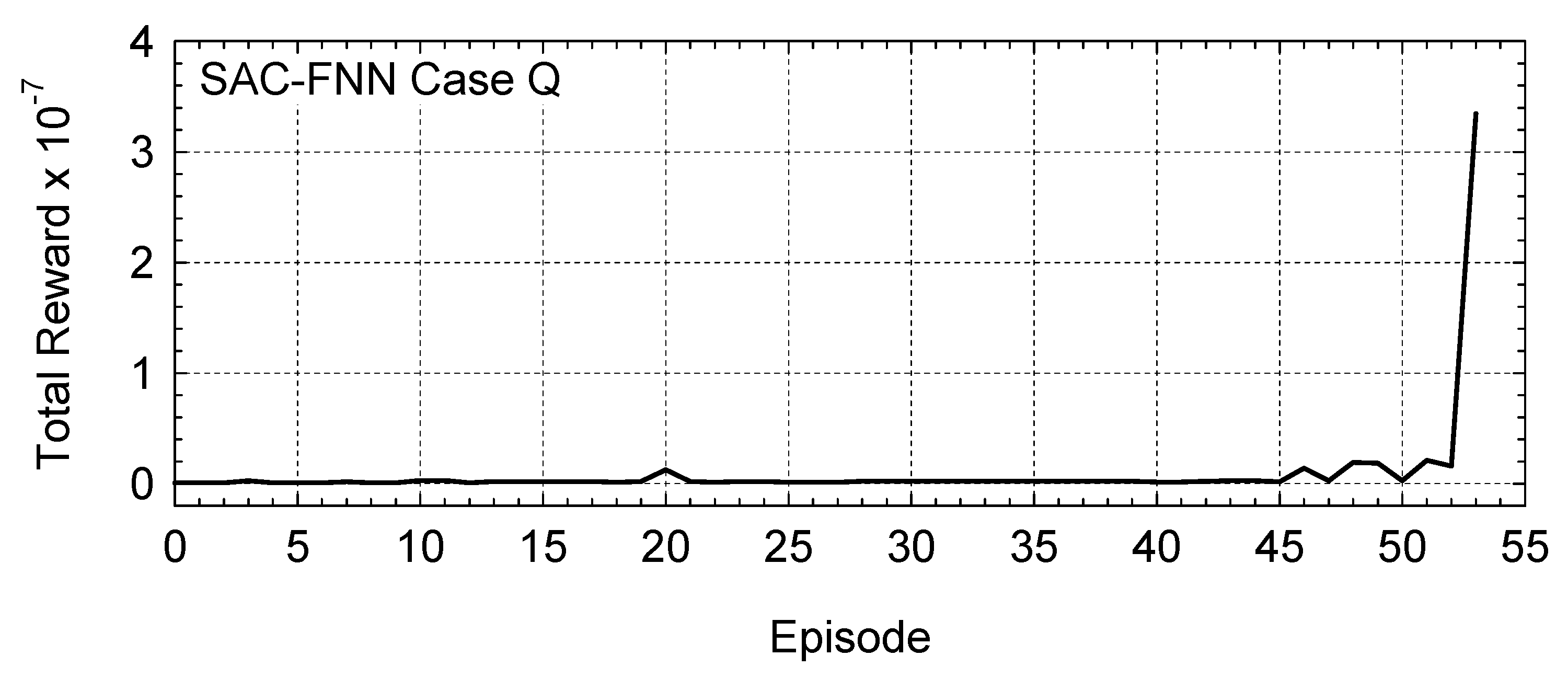
The implemented SAC-FNN algorithm performed 25 different training runs or cases, labeled A-Y. The five cases labeled A-E are for troubleshooting and optimization prior to conducting the actual training cases labeled F through Y. The selected and varied hyperparameters in the SAC-FNN training cases are listed in Appendix B. As an example of the training results, Figure 15 plots the changes in the episodic reward during the training case Q with 256 neurons per hidden layer of the FNN. The small initial reward is due to the early termination of the episodes when one of the state variables, either the reactor thermal power, the reactor Na exit temperature, or the in-vessel Na mass flow rate, continuously exceeds the specified termination range for period of 60 s. Eventually, the trained SAC-FNN algorithms successfully complete the simulated startup transient in episode 53, as indicated by the large total reward.

Not all performed training cases produced successful episodes in which the SAC-FNN algorithms complete the VSLLIM startup scenario to the final reactor power setpoint of 10.0 MW_th. Thirteen successfully trained algorithms are produced during 25 training cases of the SAC-FNN algorithm. The results of the performed parametric analyses of varying the number of neurons per layer showed that only the networks with 3 layers and 64 and 256 neurons per layer produced successful training cases. The training cases R, X, and Y with networks of 64 neurons per layer produced a total of nine successful episodes. The training cases K, P, and Q with networks of three layers and 256 neurons per layer produced four successful episodes. The training cases with networks of three layers of only 32 and 16 neurons per layer did not produce any successful episodes.

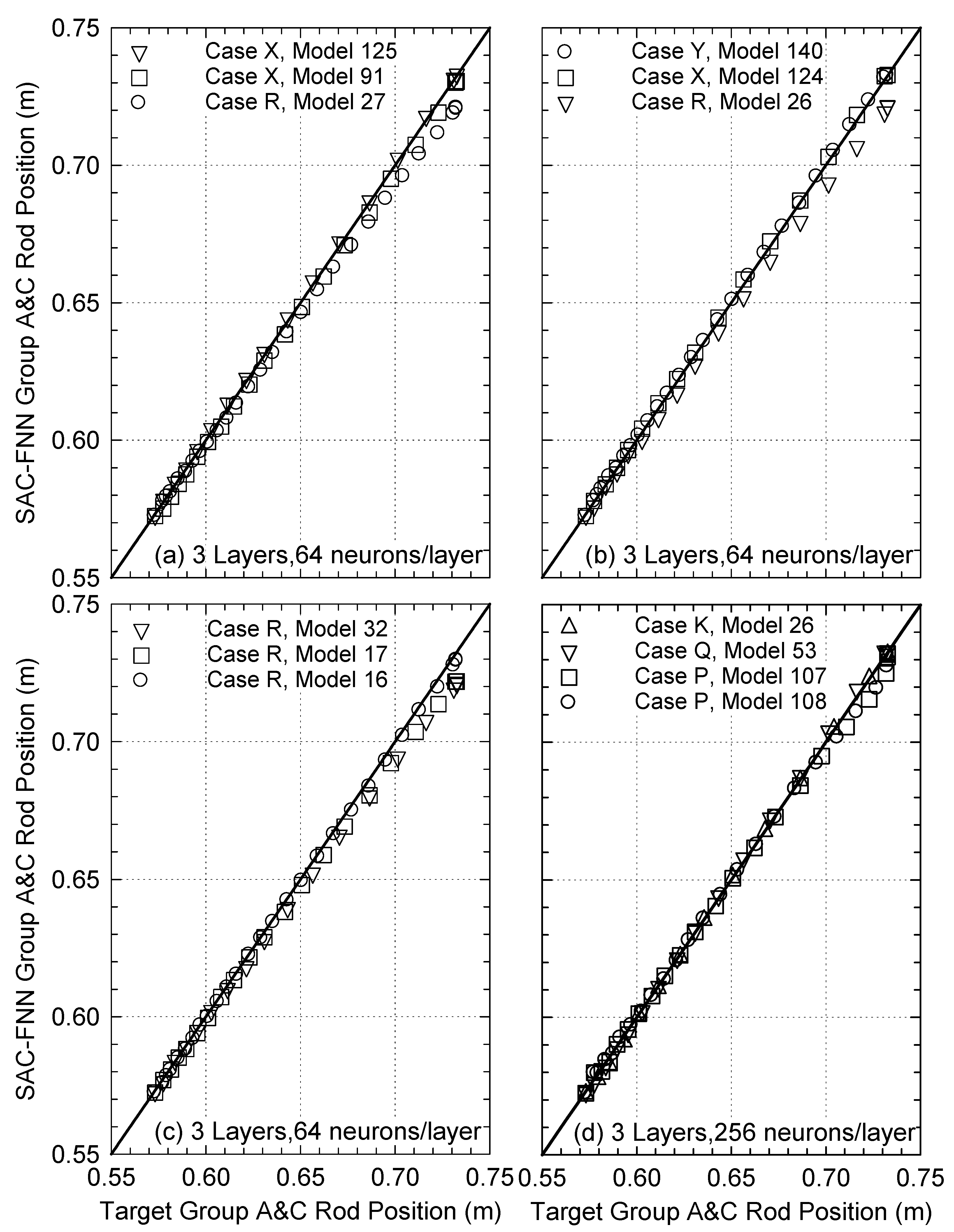
Figure 16 plots the predicted position of the Group A and C control rods in the Core of the VSLLIM microreactor by the trained SAC-FNN algorithm versus the target values in the simulated startup transients. The nine successfully trained SAC-FNN algorithms, each of three layers and 64 neurons per layer in cases R, X, and Y accurately predict the control rods’ position to within +0.3% and −1.6% of the target (Figure 16a–c). The four successfully trained SAC-FNN algorithms of three layers and 256 neurons per layer in cases K, P, and Q accurately predict the position of the control rods within +0.5% and −1.2% of the target values (Figure 16d).

To train successful models, the SAC-FNN algorithm requires more computational time than the SL-LSTM algorithm. Training the SAC-FNN algorithm with three layers and 64 neurons per layer to successfully complete the startup transient required an average of ~83 training episodes. This required an average of 54 h of computational time on an Ubuntu LTS 20.04 workstation with an AMD 3970X 32-core processor and 256 GB of RAM. The training the SAC-FNN algorithm with three layers and 256 neurons per layer required an average of ~80 training episodes with an average of 40 h of computational time. In contrast, on the same Ubuntu workstation the SL-LSTM algorithms required only 4–10 h of computational time to train a successful model. Results showed that increasing the number of neurons did not necessarily increase the required trained time.

6. Evaluating the Real-Time Controller

The trained SL-LSTM and SAC-FNN algorithms are integrated into the developed python program for the Reactor Control PLC to adjust the displacements of the control rods during the simulated startup transients using the VSLLIM digital twin model (Figure 4). During testing, the digital twin model runs synchronously to a real-time clock with a small timestep of 20 ms to produce a fine temporal discretization and a better approximation of a continuous data source. This allows the PLC to interact effectively and realistically with the VSLLIM digital twin dynamic model. The actions of the PLC are delayed by the time required for the signals of the reactor operating parameters to reach the controller, and for the generated control signals to reach the digital twin model of the reactor, providing a more realistic testing environment for the controller. In the present work the values of the state variables generated by the digital twin model of the reactor and passed on to the PLC do not include artificial sensor noise.

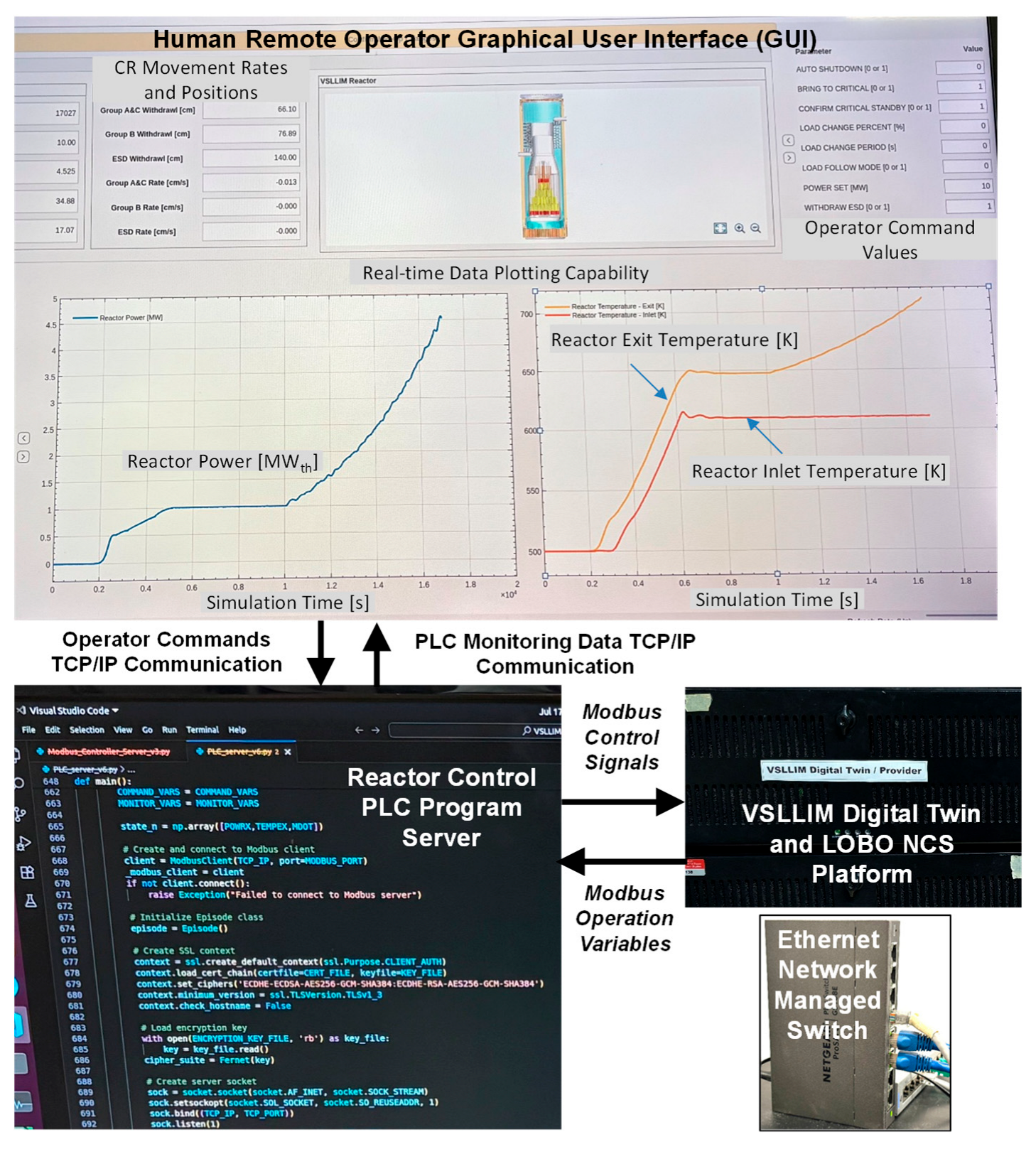
The LOBO Nuclear CyberSecurity (NCS) platform developed by University of New Mexico’s Institute for Space and Nuclear Power Studies (UNM-ISNPS) in collaboration with Sandia National Laboratory [35,36,37,38] links the Reactor Control PLC to the digital twin model of the VSLLIM reactor (Figure 4). This platform uses the Modbus Industrial Control System (ICS) protocol to manage communication through an isolated Ethernet test network. This is between the PLC program and the server running in real-time, the digital twin model of the VSLLIM microreactor (Figure 17). The controller uses two data channels, a Modbus TCP channel which communicates with the LOBO NCS platform and a TCP/IP channel, for communicating with the remote reactor operator.

The Modbus communication channel for the LOBO NCS data broker receives the calculated values of the state variables from the reactor digital twin model and stores them in Modbus holding registers (Figure 1). It also passes the Modbus control signals sent by the PLC to the digital twin model, which then enacts the transmitted control signals and displaces the control rods in the reactor core. The measured latency time of the Modbus communication between the PLC and the VSLLIM digital twin model in the ethernet testing network is ~0.2 ms on average. The TCP/IP channel receives commands from the remote operator to start up, shut down, or change the steady state setpoint for the reactor thermal power. The PLC transmits back the status of the present actions and the values of the stored state variable in the controller’s Modbus holding registers. The remote operator station has a large screen with a Graphical User Interface (GUI) for monitoring the values of state variables in real time during the simulated startup transients (Figure 17).

In each scan cycle the reactor control PLC reads the most recently received state variables in the holding registers, before passing them to the control logic program with the trained ML algorithms. They manage the movement of the Group A and C control rods in the core of the VSLLIM microreactor during the simulated startup transients using the digital twin model (Section 3.1).

The trained SL-LSTM algorithm receives an array of the values of the operation variables for the present and the previous scan cycles in the lookback window. In contrast, the trained SAC-FNN algorithm receives an array of only the present values of the operational variables. The PLC determines and implements the displacement rate of the Group A and C control rods in the core of the VSLLIM microreactor. These are commensurate with the position the rods determined by the trained algorithms. The program writes the commanded displacement rates to the Modbus holding registers of the PLC and passes them back to the LOBO NCS data broker. The data broker in turn passes the commanded movement rates to the digital twin model through a shared memory communication bridge for action. The next sections present the testing results of the trained SL-LSTM and SAC-FNN algorithms integrated with the PLC of the VSLLIM microreactor.

6.1. Results of the Control PLC with the Trained SAC-FNN Algorithm

The testing results presented in this subsection evaluate the performance of the trained SAC-FNN algorithm while integrated into the Reactor Control PLC and coupled to the digital twin model of the VSLLIM microreactor (Figure 4) using the LOBO NCS platform (Figure 17). Results are the predicted position of the control rods in the VSLLIM microreactor core by the successfully trained SAC-FNN algorithm and of the corresponding reactor thermal power determined by the digital twin model. These results are compared to those generated in the simulated startup transient of the VSLLIM microreactor connected to the PLC with the PD controller.

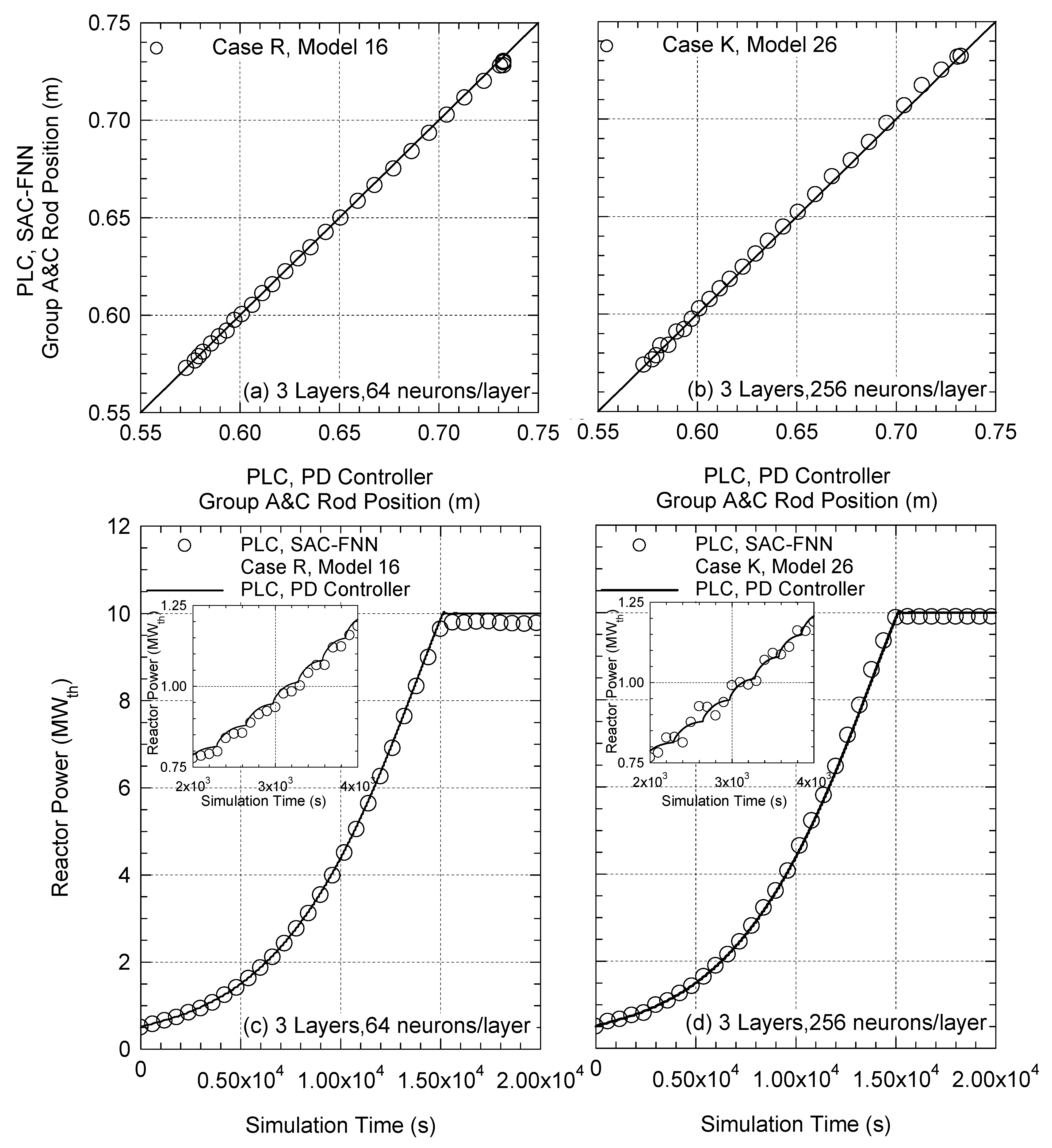
Figure 18a,b compare the predicted positions of the control rods in the cases R and K of the trained SAC-FNN algorithms of three layers of 64 and 256 neurons per layer, respectively, to those determined by the PLC with the PD controller. The PLC with the episode R trained SAC-FNN algorithm slightly underpredicts the control rod positions to within −0.6% of the values determined by the PLC with the PD controller (Figure 18a). At the end of the simulated startup transient, the reactor thermal power determined using the PLC with SAC-FNN algorithm is 9.8 MW_th compared to the target of 10.0 MW_th (Figure 18c).

The predicted positions of the control rods in the reactor core by the PLC with the episode K trained SAC-FNN algorithm of 256 neurons per layer are in good agreement, to within +0.7% and −0.5% with the values calculated using the PLC with PD controller (Figure 18b). The predictions of the PLC with the SAC-FNN algorithm levels off at a steady state reactor thermal power of 9.93 MW_th, slightly lower than the target of 10.0 MW_th (Figure 18d). The inserts in Figure 18c,d compare the small adjustments in the reactor power during the simulated startup transient. The rate limiting function Equation (1) of the PLC with the PD controller generates the target sets during training. It restricts the displacement of the control rods in Group A and C, to limit the change in the core external reactivity. Therefore, during the simulated startup transient the thermal power of the VSLLIM microreactor increases in small steps after accounting for the negative temperature reactivity feedback.

Although the PLC with the trained SAC-FNN algorithm does not have a rate limiting function Equation (1), it successfully learned to adjust the displacement of the control rods to increase the reactor power gradually without spikes (Figure 18c,d). The PLC with the trained SAC-FNN algorithm of 265 neurons per hidden layer experiences larger oscillations in the predicted reactor thermal power in the startup simulation transient to 3000 s. These oscillations are smaller for the startup transient controlled by the PLC with the trained SAC-FNN algorithm of 64 neurons per hidden layer (Figure 18c,d). Nonetheless, both algorithms in Figure 18 predict similar rates of increase of the reactor power as the reference PLC with PD controller.

During the simulated startup transient of the VSLLIM microreactor, the results in Figure 18 show that the trained SAC-FNN algorithms successfully control the movement of the Group A and C control rods (Figure 1b) to increase the reactor power from 0.5 MW_th to a final setpoint of 10 MW_th. The other eleven successfully trained SAC-FNN algorithms incorporated into the PLC demonstrated similar behaviors, as those shown in Figure 18. They smoothly increase the thermal power of the VSLLIM microreactor during the simulated startup transient to the final steady state power setpoint.

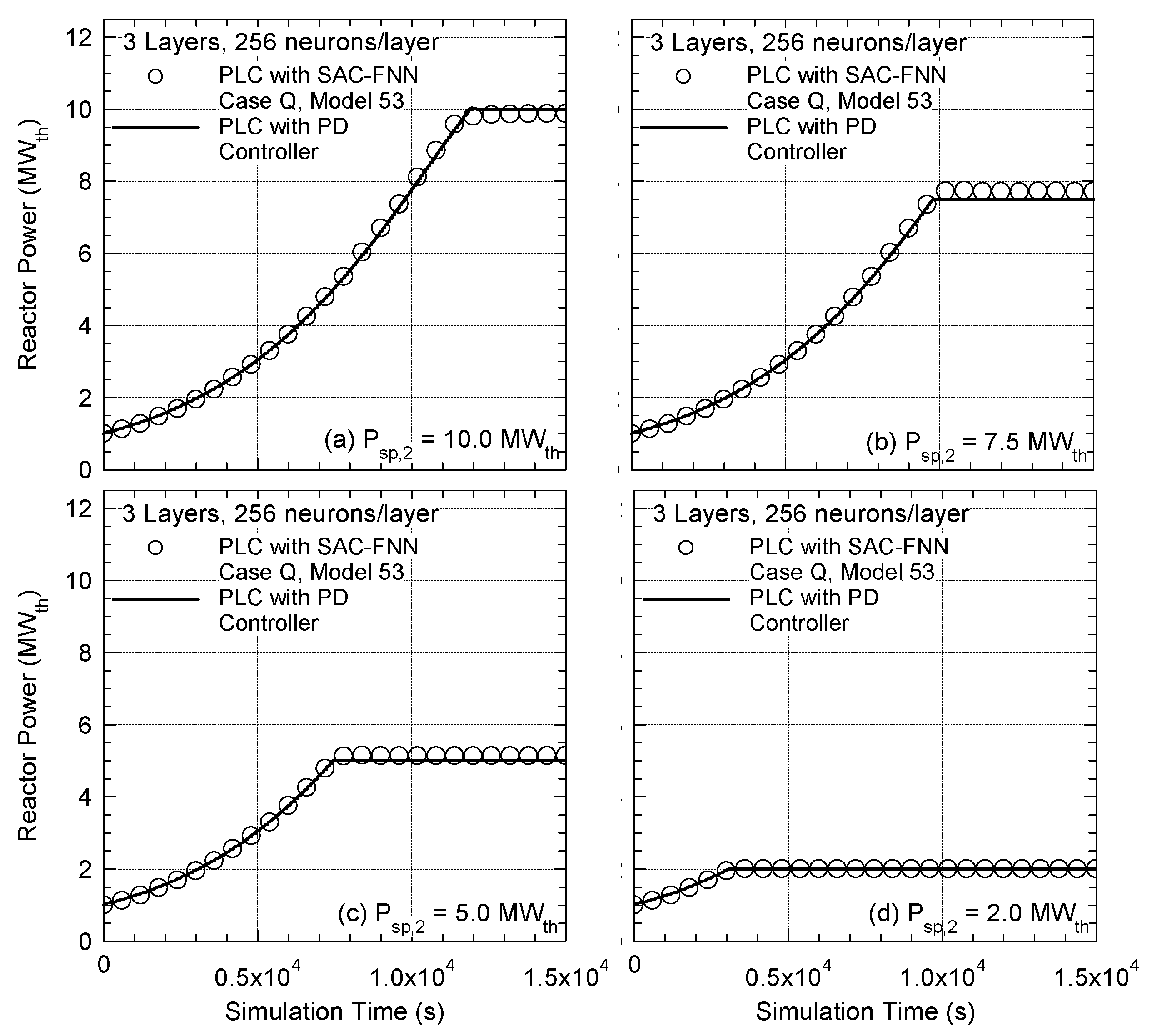
Figure 19a–d compare the calculated changes in the thermal power of the reactor controlled by PLC with the trained episode Q SAC-FNN algorithm of three layers and 256 neurons per layer in four simulated startup transients. They begin from an initial reactor power setpoint P_SP,1 = 1.0 MW_th and continue to final power setpoints, P_SP,2, of 10.0 MW_th, 7.5 MW_th, 5.0 MW_th, and 2.0 MW_th, respectively. For P_SP,2 = 10.0 MW_th the PLC with the trained SAC-FNN algorithm withdraws Group A and C control rods to increase the VSLLIM microreactor power during the simulated startup transient. During the first ~11,400 s of the simulated startup transient the reactor thermal power is close to that calculated for the reactor controlled by the PLC with PD controller. Beyond such time, and while approaching P_SP,2 = 10.0 MW_th, the predicted rate of displacement of the control rods of Group A and C in the reactor core is 1.3% lower than the value determined by the PD controller (Figure 19a).

In the simulated startup transients, the PLC with the trained SAC-FNN algorithm smoothly displaces the group A and C control rods in the reactor core (Figure 19a,b). However, the predicted final reactor power by the PLC with the trained Case Q SAC-FNN algorithm is 2.8% above the target of 7.5 MW_th (Figure 19b). In the simulated startup transients of the VSLLIM microreactor to P_SP,2 = 5.0 MW_th, the predicted final reactor power is ~2.5% higher than the target value (Figure 19c). For the lowest power setpoint of P_SP,2 = 2.0 MW_th, the prediction of the PLC with the trained SAC-FNN algorithm matches the final target power to within 0.1% (Figure 19d). It is worth noting that the trained algorithms do not display consistent bias to over or underpredict the final reactor power.

Even though the SAC-FNN algorithms in this work are trained for a single target startup scenario of increasing the reactor power from 0.5 to 10.0 MW_th, the reactor control PLC generally performs well for lower P_SP,2 values. In conclusion, the PLC with the trained SAC-FNN algorithms performs well. The predicted displacements of the Group A and C control rods in the core of the VSLLIM microreactor during the simulated startup transients are comparable to those determined by the PLC with PD controller used to generate the training data for the SAC-FNN algorithms.

6.2. Performance of the Reactor Control PLC with the Trained SL-LSTM Algorithms

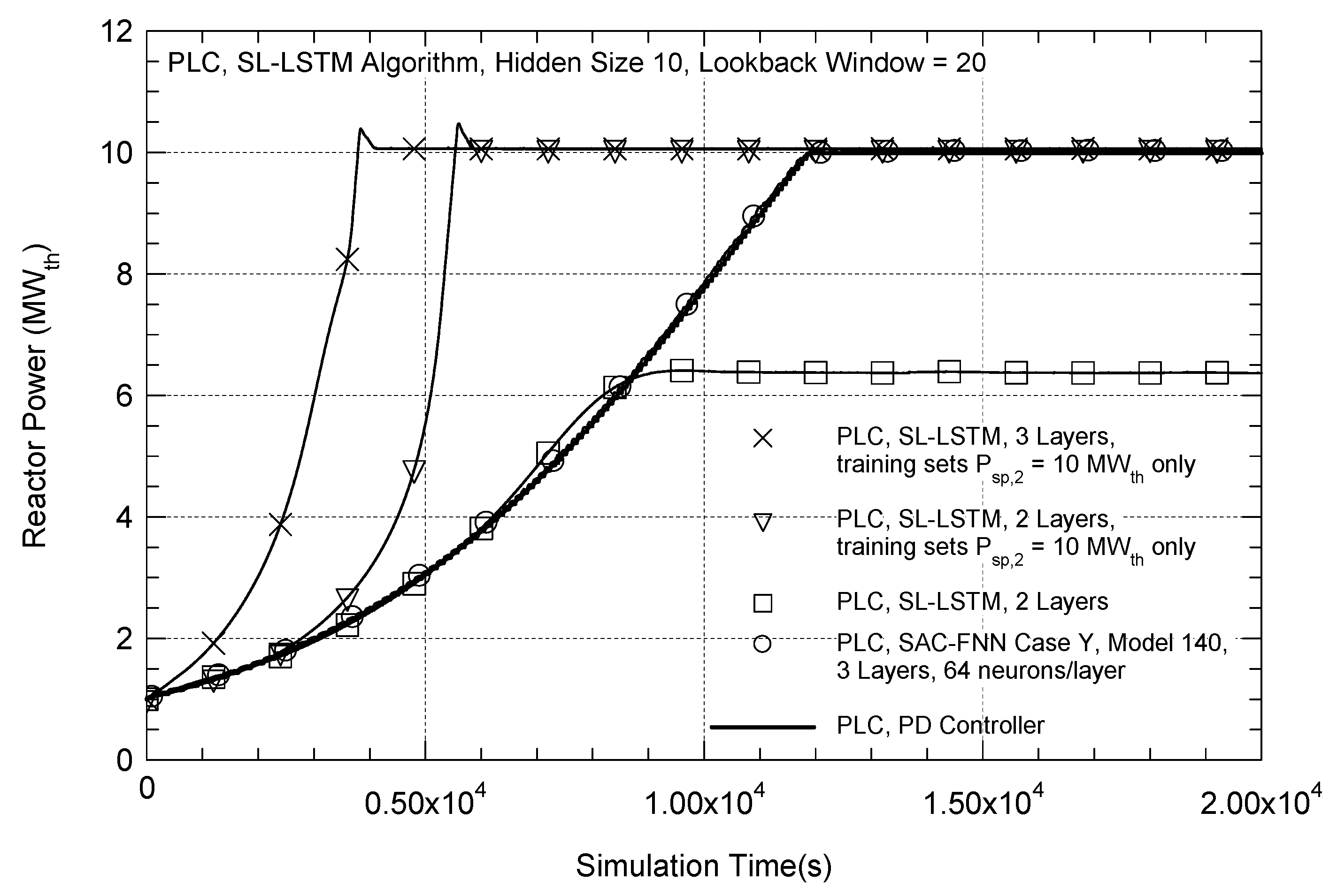
The VSLLIM Reactor Control PLC with the trained SAC-FNN algorithms performs well for real-time control of the VSLLIM microreactor. However, the performance of the PLC with the trained SL-LSTM algorithms is unsatisfactory. Figure 20 compares the predicted thermal power in a simulated startup transient using the PLC with both the trained SL-LSTM and SAC-FNN algorithms. The results presented for the trained SL-LSTM algorithms are for three different cases with a hidden size of 10 and a lookback window of 20. In the simulated startup transient, the PLC increases the reactor power from an initial value of 1.0 MW_th up to 10 MW_th.

During the first 6000 s of the simulated startup transient, the PLC with a trained SL-LSTM algorithm of two layers and the external reactivity, ρ_ex, as a feature (see Appendix A.6), increases the reactor power in good agreement with the predictions using the PD controller. However, the reactor power calculated by the digital twin model levels off at a steady state value of 6.37 MW_th, which is well below the target setpoint of 10 MW_th. The PLC and the trained SL-LSTM algorithms with two or three layers, and ρ_ex, as a feature, reach the correct reactor power setpoint of 10 MW_th. However, they rapidly displace the Group A and C control rods causing the reactor power to rise faster than the target values calculated using the PLC with PD controller.

In contrast, the PLC with the trained Case Y SAC-FNN algorithm of three layers and sixty-four neurons per layer smoothly increases the reactor power in close agreement with the predictions using the PLC with PD controller. The reactor power levels off at a steady state value of 10.02 MW_th, only 0.2% higher than the target power setpoint. This acceptable performance for the trained Case Y SAC-FNN algorithm in Figure 20 is consistent with those displayed for the Cases K, R, and Q algorithms in Figure 18 and Figure 19 for real-time control during the simulated startup transients.

The results for the Reactor Control PLC with the trained SL-LSTM algorithms show that despite the high testing accuracy of the algorithms (Figure 12a), the real-time control performance is poor and inconsistent (Figure 20). The PLC with the trained SL-LSTM algorithms does not self-correct when the values of the input features differ from those in its training data sets. Owing to the highly nonlinear kinetics of the reactor, a small change in external reactivity due to displacement of the control rods in the core results in larger changes in the reactor thermal power and, hence, the features used to train the SL-LSTM algorithm. Examples are the reactor core exit temperature and the in-vessel Na flow rate through the core by natural circulation. Despite the high testing accuracy of the SL-LSTM algorithms during training, a small difference in the predicted displacement of the control rods during real-time testing causes the reactor power to significantly deviate from the target values. The SL-LSTM algorithms do not incorporate control feedback during the training process but are trained using pre-generated data sets covering a wide range of target curves of the simulated startup transients with different reactor power setpoints. Consequently, the algorithms did not learn during training how the VSLLIM digital twin model responds to different predictions of the control rods positions from those in the training data sets. This contrasts with the trained SAC-FNN algorithms that learn to moderate the predicted displacements of the control rods and self-correct so that the increases in the reactor power agree with the target values (Figure 18, Figure 19 and Figure 20).

7. Summary and Conclusions

This work trained and investigated the performance of two different ML algorithms for remote operation and control of the VSLLIM microreactor during simulated startup transients. The trained SL-LSTM and SAC-FNN algorithms are incorporated into a PLC program for real-time control of a digital twin model of the VSLLIM reactor. The results compare the performance of the trained algorithms during training and real-time remote control of the VSLLIM microreactor. The developed physics-based MATLAB dynamic Simulink model represents that of the digital twin of this microreactor. The model generated 797 data sets for training the ML algorithms. These data sets are of the startup transients from an initial subcritical condition to different steady state power levels of the VSLLIM microreactor up to 10 MW_th.

The trained SL-LSTM algorithms predicted the position of the Group A and C control rods in the core of the VSLLIM reactor during the simulated start up transients with an accuracy of >99.90%. However, this high accuracy did not translate to good real-time control of the reactor with the PLC incorporated with the trained SL-LSTM algorithms. The PLC withdraws the control rods either too rapid or too slow, compared to targets using the PLC with PD controller. These results may be caused by the absence of feedback to adjust the predictions during the SL-LSTM algorithm training. Consequently, the PLC with the SL-LSTM algorithms do not self-correct when the state variables differ from the target values. Increasing the number of training data sets did not increase in the predictive accuracy of the SL-LSTM algorithm (Appendix A.3). Owing to the absence of feedback it is unlikely that the real-time performance of the PLC with SL-LSTM algorithms would improve with further training.

In contrast, the thirteen different trained SAC-FNN algorithms incorporated into the Reactor Control PLC successfully completed the simulated startup transients of the VSLLIM microreactor. The PLC with the trained SAC-FNN algorithms displaces the control rods for a steady rise in the reactor power that matches that of the PLC with PD controller. Four of the trained SAC-FNN algorithms that comprise three layers with 256 neurons per layer, and nine of three layers with 64 neurons per layer, performed well. Unlike the PLC with the trained SL-LSTM algorithms, those with these SAC-FNN algorithms demonstrated good real-time control of the VSLLIM microreactor. In the SAC-FNN algorithms the reward feedback for actions during training helps them to take corrective actions to adjust the reactor thermal powers to match target values during the simulated startup transients.

The predictions with thirteen trained SAC-FNN algorithms agree with the target displacement curves of the Group A and C control rods in the microreactor core to be within ±1.6%. The PLC with the nine trained SAC-FNN algorithms of 64 neurons per layer reaches 9.5% lower reactor power from the setpoint of 10.0 MW_th. The PLC with the four trained SAC-FNN algorithms of 256 neurons per layer displayed superior performance. These reach final reactor power levels that are ~0.5% higher than the setpoint of 10.0 MW_th. These trained algorithms with larger numbers of neurons learn better during the simulated startup transients and the predictions closely match the target data. The predicted final reactor powers for the PLC with the trained SAC-FNN algorithms slightly differ from the setpoint of 10.0 MW_th used during training. Nonetheless, the algorithms smoothly and accurately increase the reactor power to the target values.

In conclusion, the present research demonstrated that the trained SAC-FNN algorithms are a viable choice for remote control of the VSLLIM microreactor during simulated startup transients. The implemented PLC controller with the trained algorithms in this work can monitor the operation of the reactor and send commands to the control rod actuators, as well as communicate with a remote operator station. The remote-control function with securely encrypted and transmitted command signals and monitoring data is demonstrated in our computational laboratory at UNM-ISNPS using an isolated Ethernet network.