LGB-YOLOv11n: A Position-Specific Lightweight Detector for Shiitake Appearance Pre-Grading on Edge Devices

Abstract

Automated shiitake pre-grading in forest-understory production environments is challenged by non-uniform illumination, cluttered backgrounds, occlusion, fine-grained appearance differences, and limited edge-computing resources. This study proposes LGB-YOLOv11n, a lightweight detector that assigns modules to feature levels according to their processing roles. Large-kernel separable attention is placed at the P4/16 backbone level and P3/8 detection branch to strengthen contour, texture, edge, and local-deformation representation. Ghost modules compress the P4/16 and P5/32 detection branches, while BiFPN-inspired weighted fusion replaces four neck fusion nodes. On a held-out test set, the model achieved 97.51% mAP@0.5 and 86.62% mAP@0.5:0.95, improvements of 1.21 and 5.62 percentage points over YOLOv11n, respectively. It used 2.39 M parameters, 7.72% fewer than the baseline. Gains were retained in all three leave-one-acquisition-date-out folds, and three random-seed runs yielded 86.49% ± 0.09% mAP@0.5:0.95. Cross-domain single-class evaluation on 222 external images yielded 89.52% AP@0.5 and 63.71% AP@0.5:0.95, compared with 86.73% and 59.84% for YOLOv11n. On an NVIDIA Jetson Orin NX with TensorRT FP16, LGB-YOLOv11n achieved 134.3 ± 6.73 FPS with a mean inference pipeline latency of 7.47 ± 0.39 ms. These results demonstrate a favorable accuracy–complexity trade-off and support real-time model inference for edge-based shiitake appearance pre-grading.

1. Introduction

Shiitake (Lentinula edodes) is an important commercial mushroom. In production, preliminary appearance sorting considers visible cap plumpness, expansion state, crack density, color consistency, and overall morphology. This operation is commonly performed manually, and its consistency is affected by operator experience, illumination, target density, and batch variation. An automated pre-grading system must therefore resolve subtle interclass differences in cluttered scenes while meeting the latency, memory, and power constraints of edge hardware. The “thick” and “thin” categories used in this study are operational appearance classes derived from visible cap characteristics rather than direct measurements of physical cap thickness.

Deep-learning-based machine vision has been applied to agricultural detection and recognition tasks [1,2]. Representative applications include agricultural object counting, orchard fruit-load estimation, fruit maturity recognition, apple detection, and real-time maturity monitoring [3,4,5,6,7,8]. Convolutional neural networks have also been investigated for plant-disease recognition, with recent reviews summarizing their application scenarios, deployment trends, and current limitations [9,10,11,12].

Recent object-detection research increasingly emphasizes the joint optimization of representation quality and computational efficiency rather than accuracy alone. Two-stage detectors such as Faster R-CNN provide strong region-level modeling but introduce proposal-generation overhead [13], whereas one-stage detectors, including the YOLO family, SSD, and RetinaNet, emphasize efficient dense prediction [14,15,16,17,18,19,20,21]. Transformer-based DETR variants improve global relation modeling but can impose additional training and computational demands [22,23]. More recent real-time detectors, including YOLOX and RTMDet, further refine assignment, decoupled heads, and training strategies [24,25]. For agricultural edge systems, however, higher model capacity does not automatically translate into better field performance: the detector must preserve fine texture and boundary information while controlling parameter count, FLOPs, memory footprint, and deployment latency [1,2,26,27,28,29].

Recent mushroom-specific studies illustrate both the progress and the remaining limitations of task-oriented lightweight detection. OMC-YOLO achieved 94.95% mAP@0.5 on its oyster mushroom grading dataset while reducing parameters and computation by approximately 26% through depth-wise convolution, large-kernel attention, a lightweight neck, and loss-function modification [30]. OMB-YOLO-tiny further reduced the model to 1.72 M parameters with 90.14% mAP@0.5 for damaged Pleurotus ostreatus by combining lightweight feature extraction, feature fusion, and structured pruning [31]. These studies demonstrate that task-specific lightweighting can be effective, but their target species and decision criteria differ from the fine-grained thick/thin/malformed shiitake pre-grading considered here, and they do not jointly examine acquisition-batch robustness, cross-domain behaviour, and physical edge-device deployment.

For shiitake mushrooms, the current literature is expanding from fruiting-body detection toward grading, phenotyping, and multimodal perception. MYOLO focuses on lightweight detection of mature fresh shiitake fruiting bodies [32]. Mamba-YOLO reports 97.86% mAP@0.5 and 89.97% mAP@0.5:0.95 with 6.1 M parameters and an 8.3 ms detection time on its self-built facility-cultivation dataset [33]; nevertheless, that study identifies sensitivity to lighting variation, the absence of cross-validation, and the lack of edge-device testing as remaining limitations. Zhao et al. [34] estimate key cap traits using machine vision under structured red/green backgrounds, which is valuable for phenotyping but differs from in-field appearance grading in cluttered understory scenes. MDF-DETR introduces RGB-D information and detail-aware fusion to improve spatial perception and small/dense fruiting-body detection, but the reported 14.1 M parameters and 57.0 GFLOPs, together with the need to obtain depth information, imply a different accuracy–resource trade-off from a compact RGB-only edge detector [35]. Accordingly, published results from these different datasets should not be compared as if they shared a common benchmark; rather, they reveal complementary design directions and unresolved deployment constraints.

A second unresolved issue concerns where lightweight or context-enhancement modules should be placed. Uniformly replacing blocks at every feature level assumes that shallow, intermediate, and deep features have the same processing requirements, even though high-resolution P3 features are more sensitive to local detail loss while deeper P4/P5 features contain greater semantic abstraction and channel redundancy. Very recent YOLOv11-based mushroom research also points in the same general direction: YOLO-AREL combines lightweight downsampling, RepViT/EMA feature modeling, and an improved localization-quality head for wild-mushroom recognition, reporting a 2.0-percentage-point mAP@0.5 gain over YOLOv11n together with 23.9% fewer parameters and 19% lower GFLOPs [36]. However, its objective is multi-species wild-mushroom recognition rather than enterprise-defined shiitake appearance pre-grading, and its reported real-time test is GPU-based rather than an embedded Jetson sorting workflow. Recent LMW-YOLO work on YOLO11n, although developed for remote-sensing small-object detection rather than mushroom grading, explicitly assigns different modules to different pyramid levels and shows the methodological value of stage-specific structural design [37]. This supports treating feature-level placement as a design variable, while leaving open the application-specific question of how contextual enhancement, compression, and multi-scale fusion should be coordinated for fine-grained shiitake appearance categories under forest-understory conditions.

Based on these gaps, YOLOv11n was selected as the baseline because its compact one-stage architecture provides a suitable starting point for edge deployment while retaining P3/8, P4/16, and P5/32 multi-scale detection features [38]. The proposed LGB-YOLOv11n does not claim novelty from the individual LSA, Ghost, or weighted-fusion concepts themselves; instead, it investigates their task-oriented, position-specific coordination. LSA is placed at the P4/16 backbone level and the P3/8 detection branch to strengthen contextual representation without uniformly increasing attention operations. Ghost modules are restricted to the P4/16 and P5/32 detection branches to compress higher-level, higher-channel features while leaving the high-resolution P3 branch uncompressed. BiFPN-inspired weighted fusion (BiFPN_WF) replaces four neck fusion nodes so that the network can learn the relative contributions of aligned P3/8, P4/16, and P5/32 features. This configuration is subsequently justified through full-factorial, position-specific, and scope-specific ablations rather than by assuming that a module beneficial at one level should be applied everywhere.

The main contributions of this study are as follows:

(1)

A position-specific configuration of LSA, Ghost, and BiFPN_WF is designed for the operational appearance categories of thick, thin, and malformed shiitake mushrooms. The modules are placed at different backbone, detection-branch, and neck positions according to the feature-processing requirements of the corresponding network levels.

(2)

Full-factorial ablation experiments and position- and scope-specific comparisons are conducted to examine the effects of the three structural configurations on detection accuracy, parameter count, floating-point operations, and weight-file size. Class-wise analysis is further used to evaluate performance differences among the three appearance categories.

(3)

The final model is evaluated using a held-out test set, leave-one-acquisition-date-out validation, repeated training with different random seeds, cross-domain inference on an external evaluation set, and TensorRT FP16 deployment on the Jetson Orin NX. These experiments evaluate detection accuracy, cross-batch stability, training repeatability, cross-domain prediction behaviour, and edge-side deployment performance.

2. Materials and Methods

2.1. Image Acquisition and Annotation

The image dataset was acquired at the Huamugou forest-understory shiitake cultivation base in Keshiketeng Banner, Chifeng, Inner Mongolia, China. The cultivation site is shaded by the natural tree canopy. Image backgrounds included tree shadows, ground vegetation, and mushroom-cultivation logs, while illumination varied spatially within the acquisition scenes. Images were captured using the rear main camera of a OnePlus 11 smartphone, primarily from top-view and oblique-top-view perspectives. Data acquisition was conducted on three dates and included variation in mushroom growth state, target density, and illumination. Images containing local shadows, low illumination, occlusion, and target adhesion were retained. A total of 892 images were acquired, of which 616 were retained after quality screening. For model input, the images were resized to 640 × 640 pixels.

The shiitake instances were assigned to three operational appearance categories—thick, thin, and malformed—based on enterprise sorting experience and the manual criteria described in Section 2.2 and

Table 1. Criteria for the appearance-based classification of shiitake mushrooms.

Class	Main Visual Criteria	Annotation Rule
Thick shiitake	Plump, visibly convex cap; full or slightly curled edge; relatively dense surface texture	Manual appearance assessment; no fixed geometric threshold
Thin shiitake	Fully expanded, relatively flat cap; no evident edge curling; relatively sparse surface texture	Manual appearance assessment; no fixed geometric threshold
Malformed shiitake	Visible asymmetry, damage, adhesion, or abnormal deformation	Visible malformation takes priority over thick/thin appearance

. Two annotators used LabelImg 1.8.2 to assign category labels and draw bounding boxes. Each bounding box enclosed the complete visible portion of the mushroom cap. An occluded mushroom was annotated when approximately more than 50% of its cap remained visible. Tightly overlapping mushrooms were labeled as separate instances when their visible cap regions could be distinguished.

Annotation quality was checked using 100 randomly selected images. Disagreements between the two annotators regarding category assignment or bounding-box extent were reviewed jointly, and the corresponding annotations were revised by consensus before the dataset labels were finalized.

2.2. Operational Appearance Classes

The thick- and thin-shiitake classes used in this study were defined as operational appearance categories from monocular RGB images acquired primarily from top and oblique-top views. Labels were assigned through a joint visual assessment of apparent cap plumpness, expansion state, edge curling, texture density, local shading, and overall morphology. The definitions were designed for enterprise appearance pre-grading without relying on a single geometric threshold. Samples showing clear asymmetry, damage, adhesion, or abnormal deformation were preferentially assigned to the malformed-shiitake class. The category definitions and annotation rules are summarized in Table 1.

2.3. Dataset Split and Statistics

The dataset was split at the original-image level. The 616 retained images were divided at an 8:1:1 ratio into 493 training images, 62 validation images, and 61 test images. Data augmentation was applied only after the split and only to the training set, increasing the number of training images from 493 to 1479. The validation and test sets contained only the original images. This procedure prevented an original image and its augmented versions from being assigned to different subsets.

Table 2. Instance counts in the augmented training set and the original validation and test sets.

Class	Training Set After Augmentation	Validation Set	Test Set
Thick shiitake	10,959	473	413
Thin shiitake	8824	358	354
Malformed shiitake	3506	138	130
Total	23,289	969	897

Note: Training-set counts include augmented images, whereas validation- and test-set counts refer to original images. The corresponding average target densities are 15.75, 15.63, and 14.70 instances per image, respectively.

reports the class-wise instance counts for the augmented training set and the original validation and test sets.

The training set was used for parameter optimization, and the validation set was used for structural selection, ablation comparisons, and checkpoint selection. The held-out test set was used only for final performance evaluation after the architecture had been fixed. Although the image-level split prevented direct leakage of augmented versions across subsets, images acquired on the same date may share similar backgrounds, illumination patterns, or target clusters. A supplementary split grouped by acquisition date was therefore used to evaluate performance variation across acquisition batches, as described in Section 3.4. 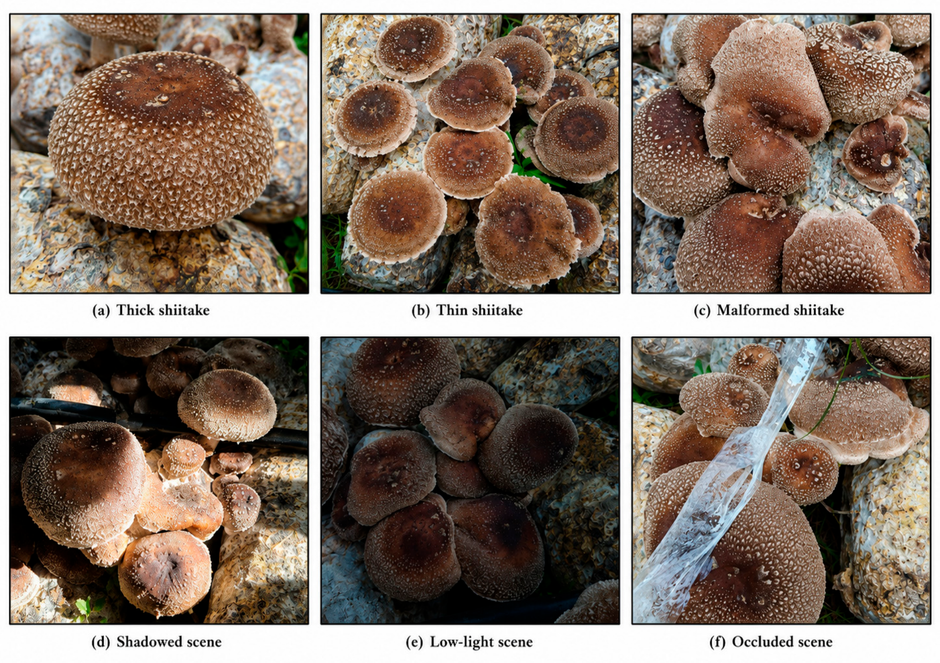Figure 1 presents example images of the three appearance categories and acquisition conditions included in the dataset.

Figure 1 illustrates the visible category characteristics and several acquisition conditions represented in the dataset. Thick shiitake typically has a plumper and more convex cap, whereas thin shiitake has a more expanded and flatter cap. Malformed samples exhibit visible asymmetry, damage, adhesion, or abnormal deformation. The dataset also includes images affected by shadows, low illumination, and target occlusion.

2.4. External Evaluation Set

An external image set was used to assess cross-domain prediction behaviour under differences in image source, background composition, imaging style, and visible illumination. The images were obtained from the public Mushroom Dataset released by Liangs on Roboflow Universe (project ID: liangs/mushroom-ggpwg) under a CC BY 4.0 license [39]. The project comprised 1007 base images and three versions. Its test split was downloaded through the Roboflow Python SDK on 26 June 2026, and 222 images were used in this study. The images included both dense and sparse target arrangements.

The external image set was not used for model training, validation, structural selection, or hyperparameter tuning. YOLOv11n and LGB-YOLOv11n were evaluated using their respective weights trained on the self-built dataset, without fine-tuning on the external images. The input size, confidence threshold, non-maximum suppression (NMS) threshold, and inference pipeline were identical for the two models and followed the settings described in Section 2.6. Because the public dataset follows a category system different from the thick-, thin-, and malformed-shiitake definitions used in this study, both the external ground-truth annotations and the three predicted shiitake categories were remapped to a single “mushroom” class for quantitative cross-domain evaluation.

After category remapping, class-agnostic NMS was applied to the merged predictions to avoid duplicate detections originating from different original category labels. Precision, Recall, AP@0.5, and AP@0.5:0.95 were then calculated on the 222 external images under the same evaluation settings for YOLOv11n and LGB-YOLOv11n. The original three-class outputs were retained only for the illustrative qualitative comparison presented later in the Section 3.

2.5. Proposed Method

2.5.1. Overall Network Structure

YOLOv11n [38] was used as the baseline detector. Its overall architecture comprises a backbone for hierarchical feature extraction, a neck for multi-scale feature fusion, and detection heads operating at different feature resolutions. LGB-YOLOv11n retains this framework while modifying selected modules at specific feature levels. In this study, position-specific configuration denotes assigning different structures to network positions associated with fine-grained feature representation, lightweight higher-level feature processing, and cross-scale fusion, rather than applying the same replacement uniformly across all levels.

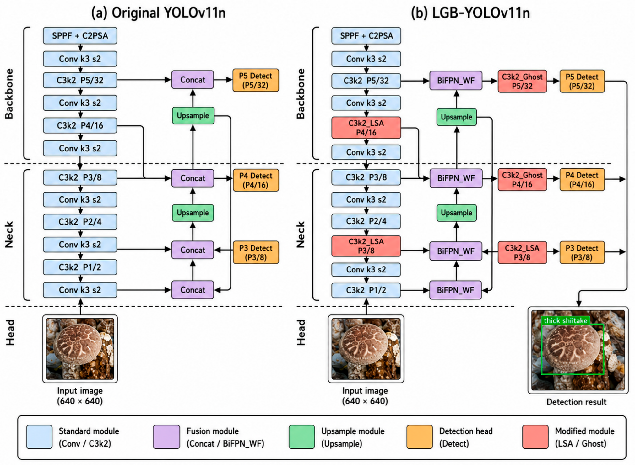
An LSA module was inserted at the P4/16 feature layer of the backbone and in the branch preceding the P3/8 detection head. Ghost modules were used in the branches preceding the P4/16 and P5/32 detection heads to reduce the parameter and computational costs of higher-level feature processing. In the neck, BiFPN_WF replaced four original feature-fusion nodes and used learnable normalized weights to combine aligned inputs from the P3/8, P4/16, and P5/32 feature levels. Figure 2 identifies these modified network positions.

Figure 2 should be interpreted as a feature-flow comparison rather than only a list of replaced blocks. For a 640 × 640 input, the baseline backbone progressively downsamples the image and produces P3/8, P4/16, and P5/32 feature levels with approximate spatial sizes of 80 × 80, 40 × 40, and 20 × 20, respectively. P3 retains the highest spatial resolution and is therefore important for small mushroom caps, local edge curvature, cracks, and partially visible regions. P4 provides an intermediate balance between spatial detail and semantic abstraction, whereas P5 has the strongest semantic abstraction and the lowest spatial resolution. The neck propagates semantic information through a top-down path and returns localization information through a bottom-up path, after which the three detection heads predict objects at the corresponding scales.

In Figure 2b, the modified modules are assigned according to these level-specific functions. The P4/16 backbone LSA enriches medium-scale contextual representation before multi-scale fusion, while the LSA in the branch preceding the P3/8 head supplements the high-resolution branch with broader context for small, occluded, or locally deformed targets. C3k2_Ghost is used only in the P4/16 and P5/32 detection branches, where channel dimensions and semantic redundancy are higher, thereby reducing computation without directly compressing the detail-sensitive P3 branch. The four BiFPN_WF nodes replace the original Concat-based fusion points in both top-down and bottom-up paths and perform normalized, learnable weighted summation after spatial/channel alignment. Thus, the architecture separates three functions—context enhancement, high-level compression, and adaptive cross-scale fusion—instead of applying one structural modification uniformly throughout the network.

2.5.2. LSA Large-Kernel Separable Attention Module

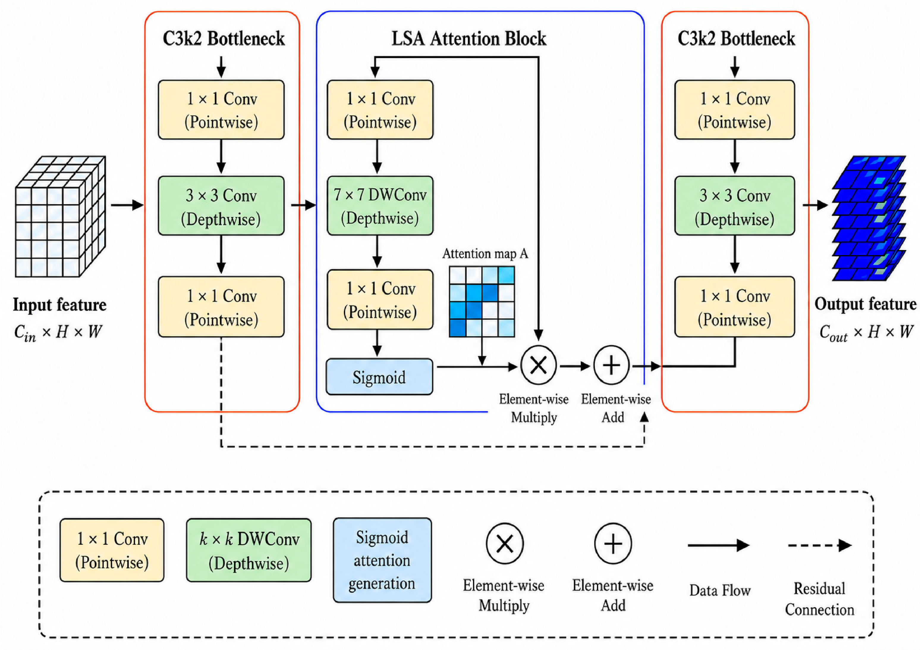
Shiitake appearance-based pre-grading relies not only on the overall cap contour, but also on fine-grained visual features such as crack distribution, edge curling, local shadows, and abnormal morphology. The effective receptive field of conventional small kernels is relatively limited, making it difficult to simultaneously capture local details and a broader spatial context. Therefore, this study introduces a large-kernel separable attention mechanism into the C3k2 structure and constructs the C3k2_LSA module, whose structure is shown in Figure 3.

Let X denote the input feature. In the tensor shown below, C_in is the number of input channels, and H and W are the spatial height and width, respectively:

$$X\in R^{C_{in}\times H\times W},$$

The input feature is first processed by the preceding C3k2 Bottleneck for local feature extraction, yielding the intermediate feature:

$$F={\beta }_1\left(X\right),$$

(1)

where β₁(·) denotes the first C3k2 Bottleneck on the left side of Figure 3, and F is the intermediate feature produced from X.

The LSA attention branch then sequentially applies a 1 × 1 pointwise convolution, a 7 × 7 depth-wise convolution, and a 1 × 1 pointwise convolution to generate the attention response. The computation is expressed as:

$$A=\sigma \left[C_{1\times 1}^{\left(2\right)}\left(D_{7\times 7}\left(C_{1\times 1}^{\left(1\right)}\left(F\right)\right)\right)\right],$$

(2)

where C_1×1⁽¹⁾(·) and C_1×1⁽²⁾(·) denote the first and second 1 × 1 pointwise convolutions, respectively; D_7×7(·) denotes the 7 × 7 depth-wise convolution; and σ(·) denotes the Sigmoid function. A is the attention map generated from F and has the same dimensions as F.

After the attention map is generated, the intermediate feature F is recalibrated by element-wise multiplication:

$$\tilde{F}=F\odot A,$$

(3)

where ⊙ denotes element-wise multiplication and $\tilde{F}$ is the recalibrated feature. To preserve the original feature representation and facilitate gradient propagation, a residual connection is then applied:

$$F_{LSA}=\tilde{F}+F=F\odot A+F,$$

(4)

Finally, the enhanced feature is processed by the subsequent C3k2 Bottleneck for further local feature extraction and channel transformation, yielding the module output:

$$Y={\beta }_2\left(F_{LSA}\right),$$

(5)

where β₂(·) denotes the second C3k2 Bottleneck on the right side of Figure 3, F_LSA is the residual-enhanced feature defined in Equation (4), and Y is the output of the C3k2_LSA module. In Y ∈ RC_out × H × W, C_out denotes the number of output channels.

The data flow in Figure 3 can therefore be summarized as follows: the first C3k2 Bottleneck extracts local features, the LSA branch generates a large-receptive-field attention map and recalibrates the intermediate feature, the residual addition retains the original information path, and the second C3k2 Bottleneck produces the final output. This arrangement enlarges contextual perception while preserving the local C3k2 processing path and avoiding the full cost of a conventional large-kernel convolution.

Compared with a standard 7 × 7 convolution, 7 × 7 depth-wise convolution performs spatial convolution independently within each channel, thereby significantly reducing the parameter count and computational overhead caused by cross-channel convolution. The preceding and following 1 × 1 pointwise convolutions are used for channel transformation and feature interaction. Thus, this module enlarges the spatial receptive field at a relatively low computational cost and adaptively enhances discriminative features through Sigmoid attention weights. The LSA used in this study is a spatial attention mechanism based on convolution-generated weight maps and differs from the query-key-value self-attention computation in Transformers. Related studies on coordinate attention, ECA, SimAM, and large receptive-field attention also indicate that low-cost feature recalibration and large-range context modeling help improve feature representation in complex visual scenes [40,41,42,43].

In this study, C3k2_LSA is deployed at the P4/16 feature layer of the backbone and the P3 detection branch. The P4/16 feature layer has both semantic abstraction capability and spatial resolution; introducing LSA at this position aims to enhance contextual representation of medium-scale appearance features such as cap contour, edge curvature, and crack distribution. The P3 detection branch retains high spatial resolution and mainly undertakes localization of small targets and local abnormal regions. Introducing LSA into this branch helps use broader contextual information to improve feature representation of damaged edges, adhered regions, occluded targets, and small mushroom caps. The joint configuration of these two positions aims to balance mid-level semantic information and high-resolution local details, and its rationality is further verified in the subsequent position ablation experiments.

2.5.3. Ghost Lightweight Module

The Ghost module [44] is a lightweight convolutional operator that first generates a small set of intrinsic feature maps and then produces additional correlated maps through inexpensive transformations. Let X be the input feature, with C_in input channels and spatial dimensions H × W:

$$X\in R^{C_{in}\times H\times W},$$

A small number of intrinsic feature maps are first generated using a 1 × 1 convolution:

$$Y=C_{1\times 1}(X;W_p), Y\in R^{m\times H\times W},$$

(6)

where C_1×1(·; W_p) denotes the 1 × 1 pointwise convolution with learnable weights W_p; the centered dot denotes a generic input, and the semicolon separates the input from the learnable parameter W_p. m is the number of intrinsic feature channels, C_out is the required output-channel number, and r is the Ghost expansion ratio. Thus, m = C_out/r. In this study, r = 2.

Subsequently, each group of intrinsic feature maps is transformed into Ghost features through a low-cost linear transformation:

$$G_i={\Phi }_i\left(Y\right), i=\mathrm{1,2},\dots ,r-1,$$

where Φ_i(·) denotes the i-th low-cost linear transformation and G_i is the corresponding generated Ghost feature group. In this study, Φ_i(·) is implemented by a 3 × 3 depth-wise convolution, and i = 1, 2, …, r − 1. Finally, the intrinsic feature Y and the generated Ghost feature groups are concatenated along the channel dimension to obtain the module output:

$$O=Concat\left[Y,{\Phi }_1\left(Y\right),{\Phi }_2\left(Y\right),\dots ,{\Phi }_{r-1}\left(Y\right)\right], O\in R^{C_{out}\times H\times W}$$

(7)

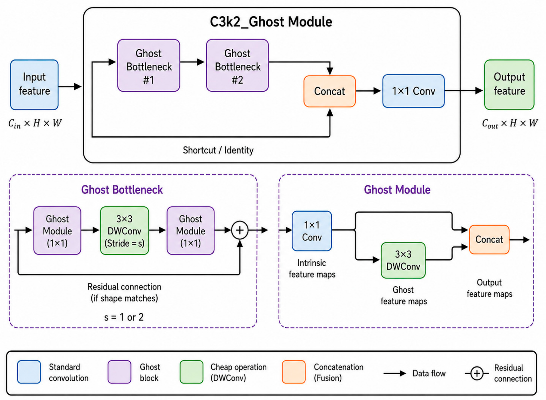
Equation (7) therefore produces C_out output channels by concatenating the intrinsic feature maps with the inexpensive Ghost feature maps. In Figure 4, the Ghost modules are embedded in Ghost Bottlenecks and then in the residual C3k2_Ghost structure. To avoid a notation conflict, the Ghost expansion ratio is denoted by r in Equations (6) and (7), whereas the symbol s shown inside the Ghost Bottleneck in Figure 4 denotes the convolution stride (1 or 2). The final LGB-YOLOv11n configuration applies C3k2_Ghost only to the P4 and P5 detection branches, while the high-resolution P3 branch remains uncompressed to preserve fine localization details.

2.5.4. BiFPN_WF Weighted Feature Fusion

The neck networks of standard YOLO series usually implement multi-scale information fusion by combining feature concatenation with subsequent convolution. However, the concatenation operation itself does not explicitly characterize the relative contribution of different input features to the fusion result. FPN [45] transmits high-level semantic information through a top-down pathway, and PANet [46] further introduces a bottom-up pathway to enhance information interaction among different levels. The BiFPN in EfficientDet [47] introduces a learnable weighted fusion mechanism based on a bidirectional feature pyramid to assign adaptive weights to input features at different scales.

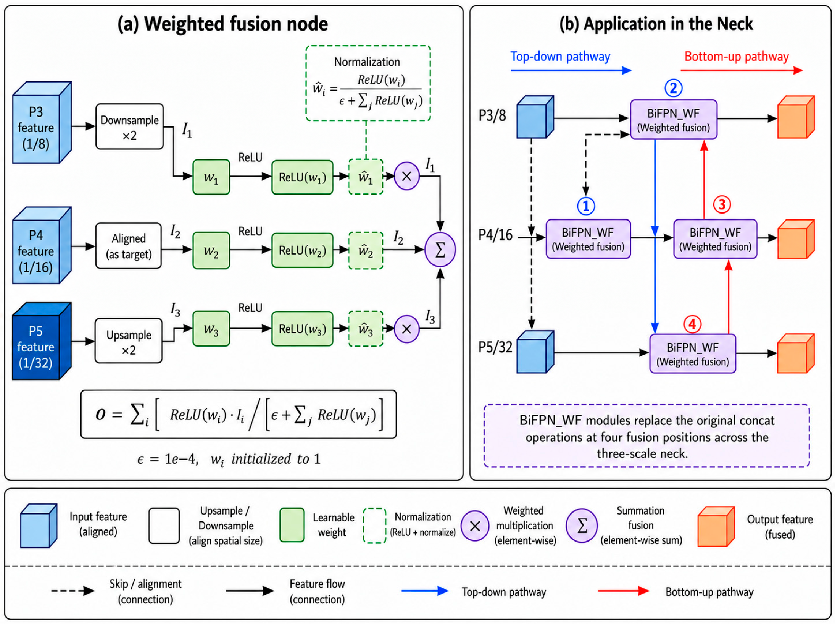
Inspired by this idea, this study constructs a BiFPN-inspired weighted feature fusion module (BiFPN_WF) and uses it to replace the four original Concat operations in the YOLOv11n neck. The four fusion positions are located in two top-down and two bottom-up pathways and involve three scales, namely P3/8, P4/16, and P5/32. Different from direct concatenation, BiFPN_WF first aligns different input features in spatial size and channel dimension, and then uses non-negative learnable weights to perform normalized weighted summation of all input features.

Let I_i denote the i-th input feature after spatial-size and channel-dimension alignment. At a given fusion node, all aligned inputs share the same channel number C and spatial dimensions H × W:

$$I_i\in R^{C\times H\times W},$$

The corresponding normalized weight is expressed as:

$$\widehat{w_i}={\displaystyle \frac{ReLU\left(w_i\right)}{\epsilon +{\sum }_j^{n}ReLU\left(w_j\right)}}$$

(8)

where w_i is the learnable scalar associated with the i-th input branch and is initialized to 1; $\widehat{w_i}$ is the corresponding normalized non-negative fusion weight; i and j index the input branches; n is the number of aligned inputs at the current fusion node; ReLU(·) constrains the raw weights to non-negative values; and ε = 10⁻⁴ is used for numerical stability. Equation (8) thus distinguishes the raw weight w_i from its normalized form $\widehat{w_i}$ .

The output of the fusion node is expressed as:

$$O={\displaystyle \sum _{i=1}^n}\widehat{w_i}{I}_i, O\in R^{C\times H\times W}$$

(9)

In Equation (9), O is the weighted fusion output and has the same aligned C × H × W dimensions as the input features I_i. The normalized weights $\widehat{w_i}$ determine the relative contribution of each input branch at the current fusion node. The fused feature is then passed to the subsequent convolutional modules for local feature extraction and channel mixing.

It should be noted that this study uses only the fast normalized weighted fusion mechanism of BiFPN and does not repeatedly stack complete bidirectional feature pyramid layers. Therefore, the fusion module is denoted as BiFPN_WF to distinguish it from the complete BiFPN network structure. Figure 5 illustrates the weighted fusion node and its application at the four neck positions.

2.6. Experimental Settings

The main experiments used a fixed random seed of 42. To evaluate training stability, three independent repeated training runs were further conducted with Seed 0, Seed 42, and Seed 3407. For prediction visualization and edge-side deployment tests, the confidence threshold and the intersection-over-union (IoU) threshold used for NMS were fixed at 0.25 and 0.45, respectively, and were kept identical for all compared models. These two thresholds were not used as fixed operating points for mAP calculation. Model performance was evaluated following the COCO protocol: AP was obtained from the area under the precision–recall curve by sweeping confidence thresholds; mAP@0.5 was calculated at IoU = 0.5, and mAP@0.5:0.95 was averaged over IoU thresholds from 0.50 to 0.95 in steps of 0.05. All models were initialized with COCO pretrained weights. In the deployment experiments, each model was first exported to an Open Neural Network Exchange (ONNX) format (opset 14) and then inferred in the TensorRT framework using 16-bit floating-point (FP16) precision with a workspace size of 4 GB [48].

Unless otherwise specified, ablation experiments used for structural selection were conducted on the validation set. During training, the checkpoint with the highest validation-set mAP@0.5:0.95 was retained for each configuration. The held-out test set was not used for module screening, structural configuration, hyperparameter tuning, or checkpoint selection. After the final architecture was fixed, the validation-selected checkpoints of YOLOv11n and LGB-YOLOv11n were evaluated on the held-out test set to generate the final test-set results reported in Section 3.

Considering the limited size of the self-built dataset and the focus of this task on fine-grained appearance differences, strong augmentation strategies such as Mosaic and MixUp were disabled during the principal training protocol to reduce excessive geometric and mosaic perturbations of shiitake texture, contour, and local morphology. Basic augmentations, including random flipping, HSV color transformation, random translation, and scale transformation, were retained. No additional class weighting or class-specific oversampling was applied. To maintain a controlled comparison of network structures, all models used the same YOLOv11n loss configuration and augmentation strategy; the influence of the lower-frequency malformed-shiitake class was examined through class-wise Precision, Recall, and AP results. The experimental configuration and main hyperparameters are listed in

Table 3. Experimental configurations and hyperparameters.

Parameter	Setting
Input size	640 × 640
Optimizer	SGD
Initial learning rate	0.01, cosine decay, lrf = 0.01
Momentum/weight decay	0.937/0.0005
Epochs/batch size	300/4
Enabled augmentation	Random flip, HSV transform, translation, scaling
Disabled augmentation	Mosaic, MixUp
Early stopping	Patience = 50
Hardware/software environment	NVIDIA GeForce GTX 1650 (4 GB VRAM) Python 3.8.20/PyTorch 2.4.1/CUDA 11.8/Ultralytics 8.3.2

. The positive-negative sample assignment strategy followed the default YOLOv11n setting.

To examine whether the principal training configuration was limited by insufficient convergence or regularization, an additional sensitivity analysis was conducted for the final LGB-YOLOv11n model. The reference setting (300 epochs; weight decay = 0.0005) was compared with (i) a longer-training configuration of 400 epochs using the same weight decay and (ii) a stronger-regularization configuration using weight decay = 0.001 with 300 training epochs. All other data splits, pretrained initialization, input size, optimizer settings, and evaluation procedures were kept unchanged. These experiments were intended to test convergence and regularization sensitivity rather than to claim global hyperparameter optimality.

To examine the influence of training-set size independently from the convergence and regularization checks, an additional learning-curve experiment was conducted for the final LGB-YOLOv11n configuration using 40%, 60%, 80%, and 100% of the original training split. Only the amount of training data was varied; the validation set, model architecture, pretrained initialization, input size, augmentation strategy, optimizer, learning-rate schedule, batch size, random seed, checkpoint-selection criterion, and evaluation protocol were kept unchanged. For each fraction, the checkpoint with the highest validation-set mAP@0.5:0.95 was retained.

For the Jetson Orin NX deployment experiment, the reported end-to-end inference pipeline latency was defined as the elapsed time for image pre-processing, TensorRT FP16 engine inference, and prediction post-processing including non-maximum suppression (NMS). FPS was derived from the same per-image pipeline timing measurements as reciprocal throughput, so latency and FPS describe the same measured processing path.

3. Results

3.1. Main Ablation Experiment

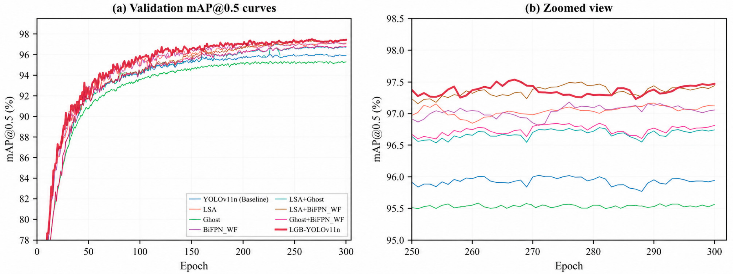
A three-factor, two-level full-factorial ablation design with eight configurations was used to examine the individual and combined effects of C3k2_LSA, C3k2_Ghost, and BiFPN_WF. YOLOv11n served as the baseline, and the data split, training strategy, and remaining hyperparameters were held constant. Figure 6 shows the validation mAP@0.5 trajectories, while

Table 4. Full-factorial ablation results for the three structural configurations on the validation set.

Configuration	mAP@0.5 (%)	mAP@0.5:0.95 (%)	Params (M)	FLOPs (G)	Weight Size (MB)
YOLOv11n baseline	96.03	80.44	2.59	6.40	5.20
LSA	97.16	84.79	2.59	6.40	5.20
Ghost	95.62	79.74	2.39	6.20	4.80
BiFPN_WF	97.19	83.32	2.59	6.40	5.20
LSA + Ghost	96.74	82.54	2.39	6.20	4.80
LSA + BiFPN-WF	97.44	86.68	2.59	6.40	5.20
Ghost + BiFPN-WF	96.81	84.23	2.39	6.20	4.80
LGB-YOLOv11n	97.54	86.40	2.39	6.20	4.80

Note: LSA was deployed at the P4/16 feature layer of the backbone and the P3 detection branch; Ghost was deployed in the P4 and P5 detection branches; and BiFPN_WF was deployed at the four feature-fusion nodes of the neck. All accuracy results in this table were obtained on the validation set during structural selection. After the configuration was fixed, the final model was independently evaluated on the held-out test set, and the corresponding test-set results are reported later in the held-out test-set comparison.

reports the corresponding validation accuracy and structural-complexity results used for model selection.

As shown in Table 4, LSA alone increased mAP@0.5 and mAP@0.5:0.95 from 96.03% and 80.44% to 97.16% and 84.79%, respectively. Ghost alone reduced the parameter count, FLOPs, and weight-file size by 7.72%, 3.13%, and 7.69%, respectively, but decreased mAP@0.5:0.95 by 0.70 percentage points. BiFPN_WF alone increased mAP@0.5 and mAP@0.5:0.95 by 1.16 and 2.88 percentage points. The validation trajectories in Figure 6 show that the configurations stabilized at different performance levels during the later training epochs, with the complete model remaining among the highest-performing configurations.

Among the two-component combinations, LSA + BiFPN_WF achieved the highest mAP@0.5:0.95 value of 86.68%. Adding Ghost produced the complete LGB-YOLOv11n model, which achieved the highest mAP@0.5 value (97.54%) and an mAP@0.5:0.95 of 86.40%, 0.28 percentage points below LSA + BiFPN_WF, while reducing the parameter count, FLOPs, and weight-file size to 2.39 M, 6.20 G, and 4.80 MB. Relative to the YOLOv11n baseline, the complete configuration increased mAP@0.5 and mAP@0.5:0.95 by 1.51 and 5.96 percentage points and reduced all three complexity indicators.

3.2. Ablation on Module Deployment Position and Structural Scope

To analyze the influence of module deployment position and structural replacement scope on model performance, ablation experiments were conducted for the insertion position of LSA, the compression position of Ghost, and the replacement scope of BiFPN_WF. The accuracy and model complexity of hierarchical configurations and expanded deployment scopes were compared.

First, the insertion position of LSA was varied under the Ghost + BiFPN_WF framework, and the validation-set results are shown in

Table 5. Ablation results for LSA deployment positions.

Model	LSA Position	mAP@0.5 (%)	mAP@0.5:0.95 (%)	Params (M)
Ghost + BiFPN, no LSA	None	96.81	84.23	2.390
LSA-P4	Backbone P4/16	97.03	85.07	2.391
LSA-P3	P3 detection branch	97.14	85.64	2.393
LSA-P4 + P3	Backbone P4/16 + P3	97.54	86.40	2.394
LSA-P3 + P4 + P5	All detection branches	97.26	86.12	2.396

.

Table 5 shows that, under the Ghost + BiFPN_WF framework, inserting LSA at P4/16 or P3 increased mAP@0.5:0.95, with a larger increase for the P3 branch. Joint deployment at P4/16 and P3 produced the highest value of 86.40%. Extending LSA to all detection branches reduced mAP@0.5:0.95 to 86.12%, so the broader deployment scope did not improve the validation result under the current dataset and configuration.

Second, under the LSA + BiFPN_WF framework, C3k2 modules in different detection branches were replaced separately, and the validation-set results are shown in

Table 6. Ablation results for Ghost deployment positions.

Model	Ghost Position	mAP@0.5 (%)	mAP@0.5:0.95 (%)	Params (M)
LSA + BiFPN, no Ghost	None	97.44	86.68	2.59
Ghost-P3	P3 branch	96.56	84.61	2.45
Ghost-P4	P4 branch	97.30	86.10	2.49
Ghost-P5	P5 branch	97.25	85.98	2.50
Ghost-P4 + P5	P4 + P5 branches	97.54	86.40	2.39
Ghost-P3 + P4 + P5	All detection branches	97.12	85.88	2.26

.

As shown in Table 6, placing Ghost in the P3 branch reduced mAP@0.5:0.95 to 84.61%. Placement in only the P4 or P5 branch yielded 86.10% and 85.98%, respectively. Joint replacement of P4 and P5 reduced the parameter count from 2.59 M to 2.39 M, increased mAP@0.5 from 97.44% to 97.54%, and changed mAP@0.5:0.95 from 86.68% to 86.40%. Replacing all three branches further reduced the parameter count to 2.26 M but lowered mAP@0.5:0.95 to 85.88%. The P4+P5 configuration was therefore retained for the final model.

Finally, the performance of BiFPN_WF was compared when applied to partial fusion nodes, all four fusion nodes, and a repeatedly stacked BiFPN structure. The validation-set results are shown in

Table 7. Ablation results for the replacement scope of BiFPN_WF.

Model	Fusion Scope	mAP@0.5 (%)	mAP@0.5:0.95 (%)	Params (M)	FLOPs (G)
LSA + Ghost, no BiFPN	Original Concat	96.74	82.54	2.39	6.20
Top-down only	2 top-down nodes	96.78	84.33	2.39	6.20
Bottom-up only	2 bottom-up nodes	96.62	84.08	2.39	6.20
Four-node weighted fusion	4 fusion nodes	97.54	86.40	2.39	6.20
Full stacked BiFPN	Repeated bidirectional BiFPN	97.55	87.10	2.52	7.60

.

Table 7 shows that replacing only the top-down or bottom-up fusion nodes improved mAP@0.5:0.95, although the improvement was smaller than that obtained with the four-node configuration. When weighted fusion was applied to all four nodes, mAP@0.5:0.95 increased from 82.54% to 86.40%, while FLOPs remained 6.20 G at the reported precision. The repeatedly stacked BiFPN further increased mAP@0.5:0.95 to 87.10%, but the parameter count and FLOPs increased to 2.52 M and 7.60 G, respectively. Considering detection accuracy and computational complexity, the four-node BiFPN_WF configuration was adopted.

Across the position- and scope-specific comparisons, extending LSA or Ghost to all detection branches did not improve the selected validation metric. Under the current task, the position-specific configuration provided a more favorable accuracy–complexity result than uniformly expanding the replacement scope. This conclusion is limited to the evaluated architecture, data split, and training settings.

3.3. Comparison with Mainstream Object Detectors

Because inference speed in frames per second (FPS) is strongly affected by the inference backend, hardware platform, and post-processing implementation, detection accuracy and structural complexity are reported separately from the Jetson Orin NX TensorRT deployment results.

Table 8. Performance comparison with mainstream object detectors.

Model	Precision (%)	Recall (%)	mAP@0.5 (%)	mAP@0.5:0.95 (%)	Params (M)	FLOPs (G)	Weight (MB)
YOLOv5n	85.63	81.27	91.37	76.83	2.19	5.9	4.42
YOLOv5m	89.57	84.86	93.27	78.63	22.14	49.00	42.57
YOLOv8n	87.53	82.17	92.73	78.87	2.69	6.90	5.35
YOLOv8m	93.07	89.56	95.63	82.47	23.22	67.80	44.60
YOLOv10n	81.73	77.93	90.63	76.57	2.71	8.40	5.47
YOLOv10m	91.07	86.53	94.23	81.27	16.49	64.00	31.92
YOLOv11n	94.45	92.69	96.30	81.00	2.59	6.40	5.20
YOLOv12n	92.57	88.53	95.27	80.83	2.60	6.50	5.30
YOLOv9t	95.23	92.07	95.17	79.57	2.00	7.70	4.10
YOLOv11n+SE	96.23	93.27	96.18	81.33	2.62	6.55	5.35
YOLOv11n+CBAM	96.47	93.53	96.42	82.13	2.65	6.60	5.40
LGB-YOLOv11n	97.45	93.85	97.51	86.62	2.39	6.20	4.80

reports Precision, Recall, mAP, parameter count, floating-point operations (FLOPs), and weight-file size for each model on the held-out test set. The detection metrics were obtained using the final validation-selected checkpoints under a unified test protocol, whereas edge-side real-time performance was evaluated separately in Section 3.9 using a unified TensorRT FP16 deployment protocol.

To evaluate the overall performance of the proposed method, LGB-YOLOv11n was compared with lightweight and medium-scale detectors, including YOLOv5n/m, YOLOv8n/m, YOLOv10n/m, YOLOv11n, YOLOv12n, and YOLOv9t. SE and CBAM were included as representative attention-based baselines to compare the position-specific configuration with general-purpose attention enhancement. All models were trained and tested using the same data split, input size, training epochs, and evaluation protocol [18,38,49,50,51,52,53,54].

Table 8 shows that LGB-YOLOv11n achieved Precision, Recall, mAP@0.5, and mAP@0.5:0.95 values of 97.45%, 93.85%, 97.51%, and 86.62%, respectively, on the held-out test set. These values exceeded the YOLOv11n baseline by 3.00, 1.16, 1.21, and 5.62 percentage points. The parameter count, FLOPs, and weight-file size were 2.39 M, 6.20 G, and 4.80 MB, respectively, all lower than those of the baseline. 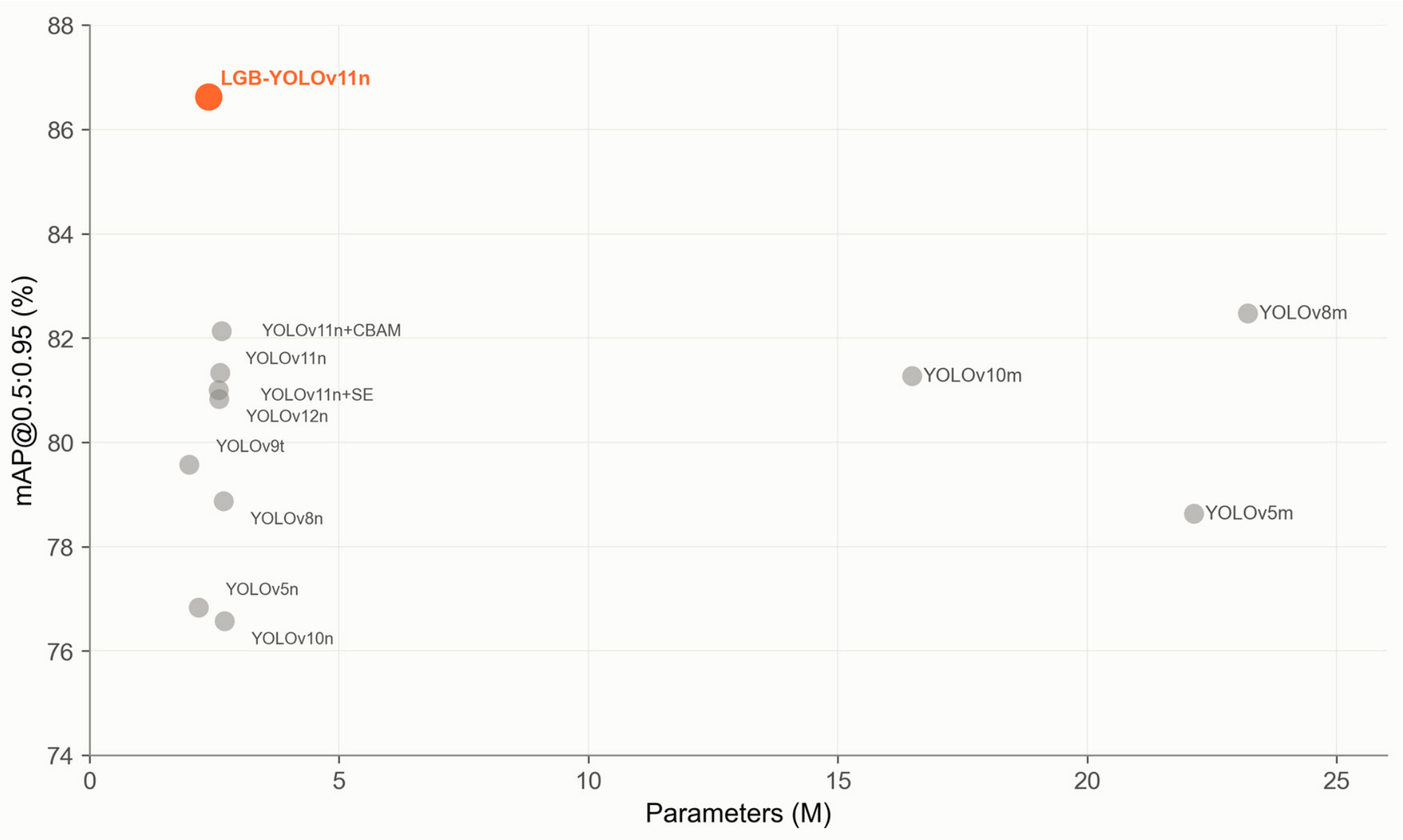Figure 7 visualizes the accuracy–parameter relationship: LGB-YOLOv11n occupies the high-accuracy, low-parameter region of the comparison, whereas the medium-scale models require 16.49–23.22 M parameters and yield lower mAP@0.5:0.95 values under the same test protocol.

Across the evaluated detector families, increasing model scale from nano/tiny to medium variants generally raised Precision, Recall, and mAP, but with a disproportionate increase in structural complexity. For YOLOv8, mAP@0.5:0.95 increased from 78.87% for YOLOv8n to 82.47% for YOLOv8m, while the parameter count increased from 2.69 M to 23.22 M and FLOPs from 6.90 G to 67.80 G; YOLOv10 showed a similar accuracy–complexity pattern. Among the compact models, a lower parameter count did not necessarily correspond to higher accuracy: YOLOv9t used 2.00 M parameters but achieved 79.57% mAP@0.5:0.95. The SE- and CBAM-enhanced YOLOv11n variants provided moderate accuracy improvements with slightly increased complexity, whereas LGB-YOLOv11n increased Precision, Recall, mAP@0.5, and mAP@0.5:0.95 while reducing the parameter count, FLOPs, and weight-file size relative to the YOLOv11n baseline.

3.4. Cross-Acquisition-Date Validation

The 616 retained images were acquired on three dates. To examine performance under acquisition-batch separation and reduce the influence of scene similarity across subsets, a leave-one-acquisition-date-out experiment was conducted. In each fold, data from two dates formed the training source, 10% of which was reserved for validation, while the remaining date was used as the test set. All folds used the pretrained weights, input size, training hyperparameters, and evaluation protocol described in Section 2.6. The fold-specific results are reported in

Table 9. Batch-wise split validation results.

Model	Fold 1 (Day 3 Test)	Fold 2 (Day 2 Test)	Fold 3 (Day 1 Test)	Mean ± SD	Random-Split Validation (Reference)
YOLOv11n baseline	77.2	76.8	77.8	77.3 ± 0.5	80.44
LGB-YOLOv11n	84.1	83.7	84.5	84.1 ± 0.4	86.40

.

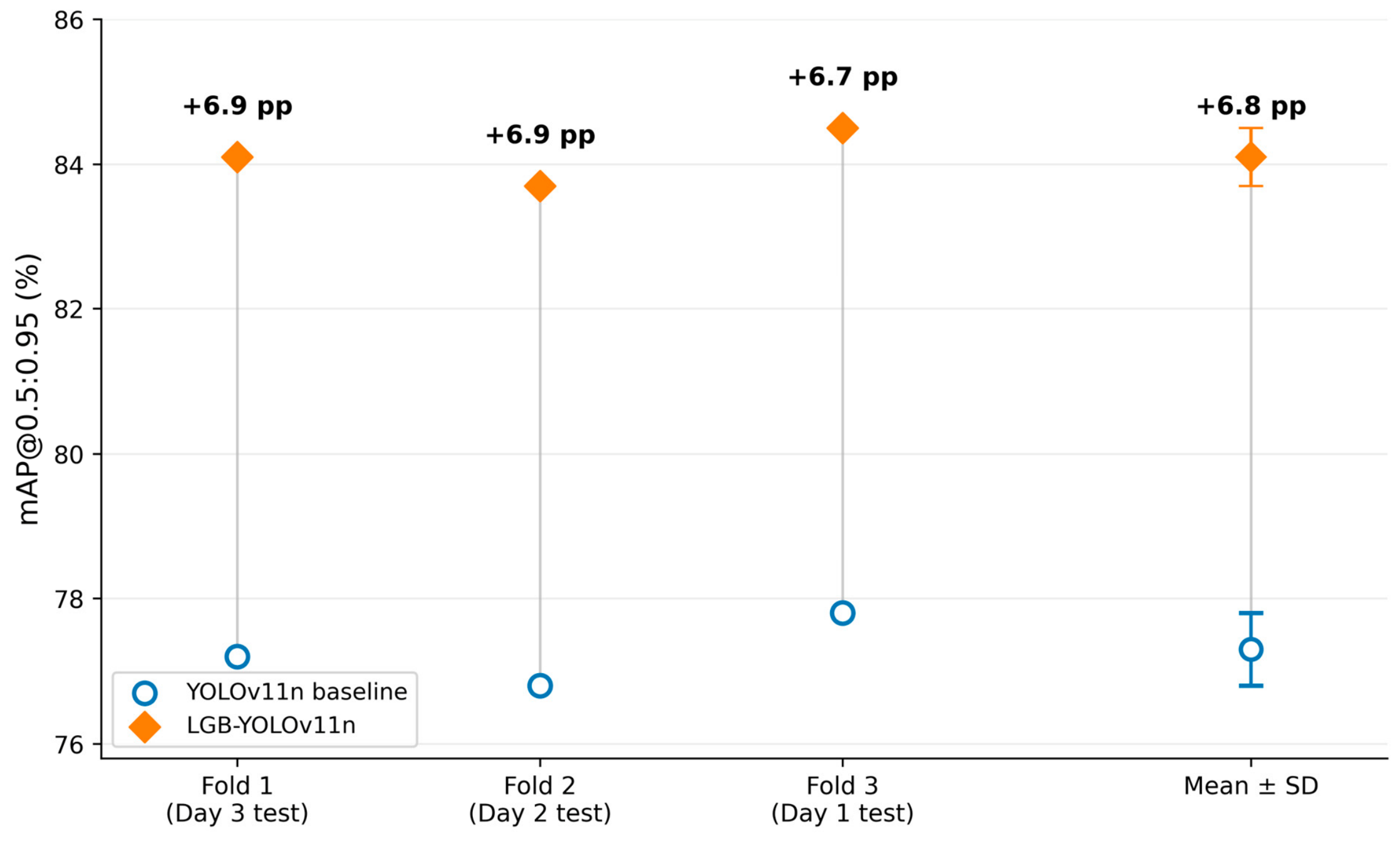
Under the leave-one-acquisition-date-out split, LGB-YOLOv11n achieved a mean mAP@0.5:0.95 of 84.1% ± 0.4%, compared with 77.3% ± 0.5% for YOLOv11n. The gains were 6.9, 6.9, and 6.7 percentage points in the three folds, as summarized in Figure 8. Performance was lower than under the random split, indicating acquisition-date variation, while LGB-YOLOv11n maintained a gain over the baseline in every fold.

3.5. Cross-Domain Inference Analysis on the External Evaluation Set

The external image set enabled cross-domain evaluation under differences in image source, background composition, viewpoint, target density, and visible illumination. It had no image overlap with the self-built training, validation, or test sets and was not used for model selection or threshold adjustment. Both models were applied without fine-tuning. For quantitative evaluation, all external annotations and the thick, thin, and malformed predictions were remapped to a single “mushroom” class, followed by class-agnostic NMS. Precision, Recall, AP@0.5, and AP@0.5:0.95 were calculated using identical settings for both models.

After single-class remapping, LGB-YOLOv11n obtained a Precision of 87.16%, Recall of 83.47%, AP@0.5 of 89.52%, and AP@0.5:0.95 of 63.71%, compared with 84.32%, 80.15%, 86.73%, and 59.84% for YOLOv11n, respectively. The corresponding gains were 2.84, 3.32, 2.79, and 3.87 percentage points. These values provide a quantitative measure of cross-domain detection performance without external-set fine-tuning.

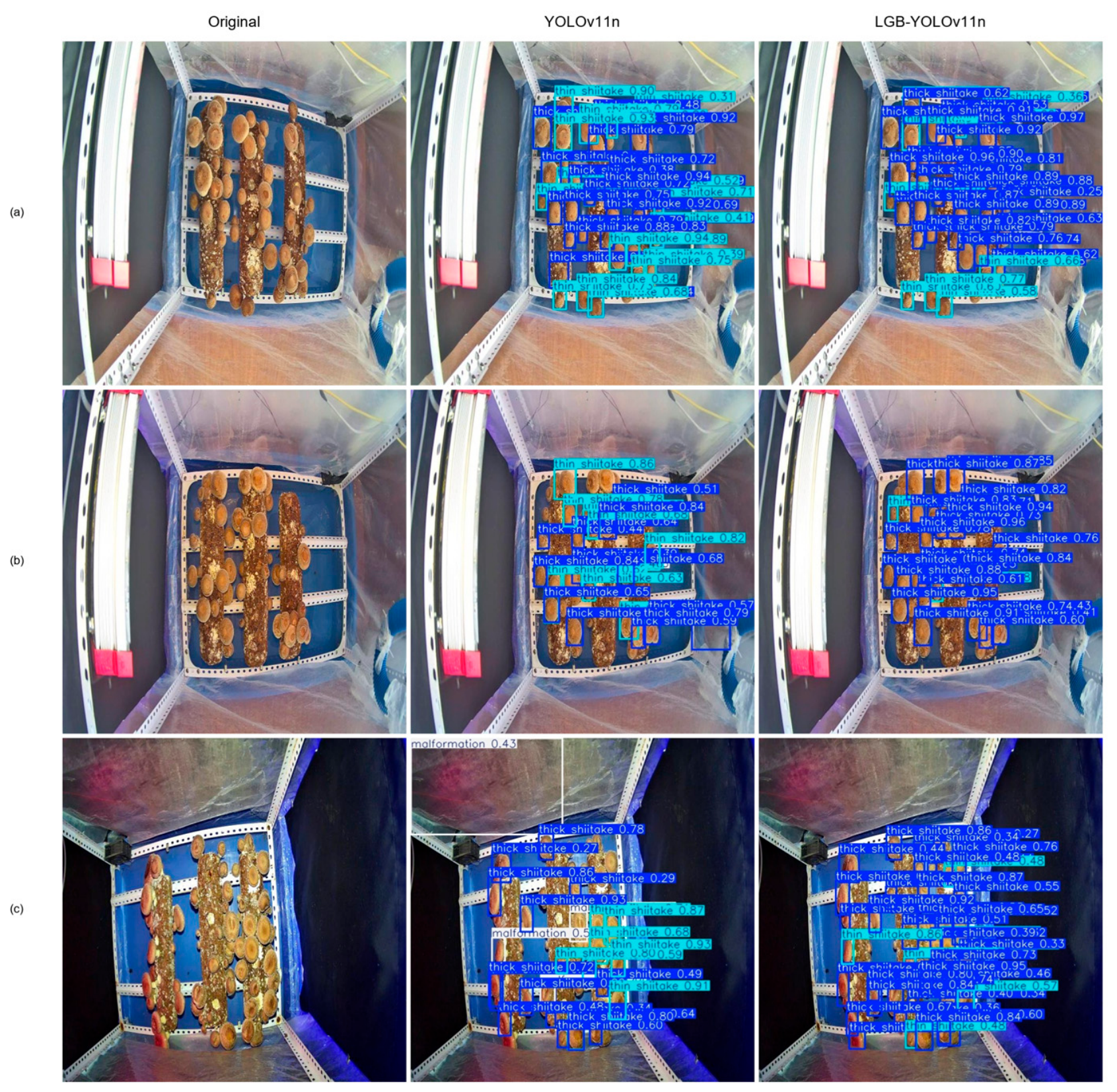
Figure 9 presents three illustrative external samples containing dense targets, partial occlusion, overlapping cap boundaries, viewpoint variation, non-uniform illumination, and lighting-color changes. The panels show the original image and the predictions of the two models under identical inference settings. Differences in missed, redundant, and class-assignment predictions can be visually inspected alongside the quantitative single-class results reported in

Table 10. Single-class cross-domain quantitative evaluation on the 222-image external dataset.

Model	Precision (%)	Recall (%)	AP@0.5 (%)	AP@0.5:0.95 (%)
YOLOv11n baseline	84.32	80.15	86.73	59.84
LGB-YOLOv11n	87.16	83.47	89.52	63.71

.

3.6. Random-Seed Stability Analysis

To examine sensitivity to random initialization, YOLOv11n and LGB-YOLOv11n were each trained using Seed 0, Seed 42, and Seed 3407. The mean mAP@0.5:0.95 values were 80.20% ± 0.21% and 86.49% ± 0.09%, respectively. LGB-YOLOv11n exceeded the baseline in all three runs, and the corresponding standard deviations were 0.21 and 0.09 percentage points.

3.7. Training-Convergence, Regularization, and Training-Set-Size Sensitivity

Table 11. Training-convergence and regularization sensitivity of LGB-YOLOv11n on the validation set.

Setting	Epochs	Weight Decay	Best Epoch	mAP@0.5:0.95 (%)
Reference	300	0.0005	268	86.40
Longer training	400	0.0005	327	86.52
Stronger regularization	300	0.001	281	86.47

summarizes the additional sensitivity experiments for the final LGB-YOLOv11n model. The 300-epoch reference configuration achieved 86.40% mAP@0.5:0.95, with the best checkpoint at epoch 268. Extending training to 400 epochs yielded 86.52%, with the best checkpoint at epoch 327, while the stronger-regularization configuration (weight decay = 0.001, 300 epochs) yielded 86.47%, with the best checkpoint at epoch 281.

The sensitivity results are reported here as a bounded check of convergence and regularization under the evaluated settings. They are not intended to establish a globally optimal hyperparameter configuration.

To evaluate model performance as a function of training-set size, the final LGB-YOLOv11n configuration was trained with 40%, 60%, 80%, and 100% of the original training split under the controlled protocol described in Section 2.6.

Table 12. Training-set-size learning-curve results of LGB-YOLOv11n on the validation set.

Training-Set Fraction (%)	Best Epoch	mAP@0.5:0.95 (%)
40	238	81.72
60	251	83.91
80	259	85.34
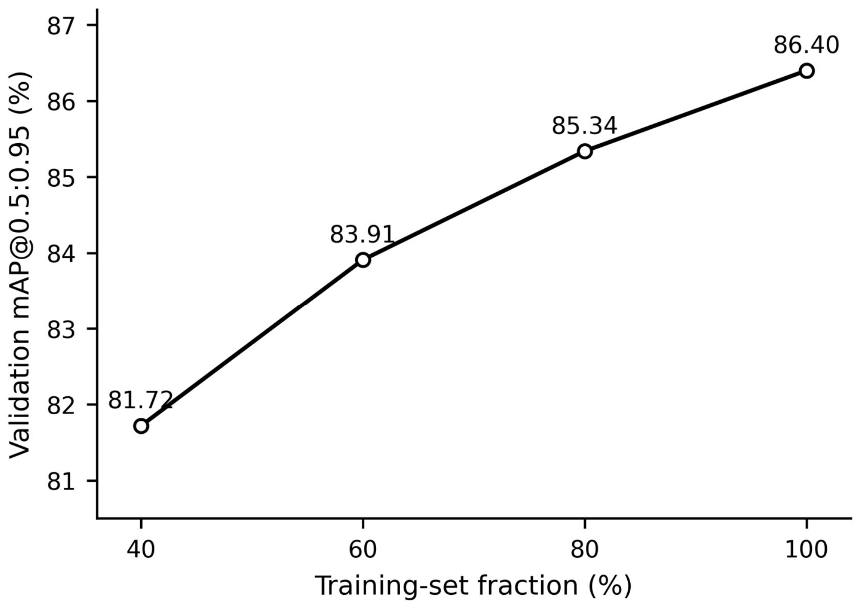
100	268	86.40

reports the best validation checkpoint for each fraction, and Figure 10 shows the corresponding learning curve.

Validation mAP@0.5:0.95 increased from 81.72% at 40% of the training set to 83.91%, 85.34%, and 86.40% at 60%, 80%, and 100%, respectively. The corresponding best epochs were 238, 251, 259, and 268. The absolute gain associated with each additional 20 percentage points of training data decreased from 2.19 to 1.43 and then to 1.06 percentage points. Thus, performance continued to benefit from additional training images, but the incremental improvement became progressively smaller as the full training set was approached.

3.8. Class-Wise Detection Performance Analysis

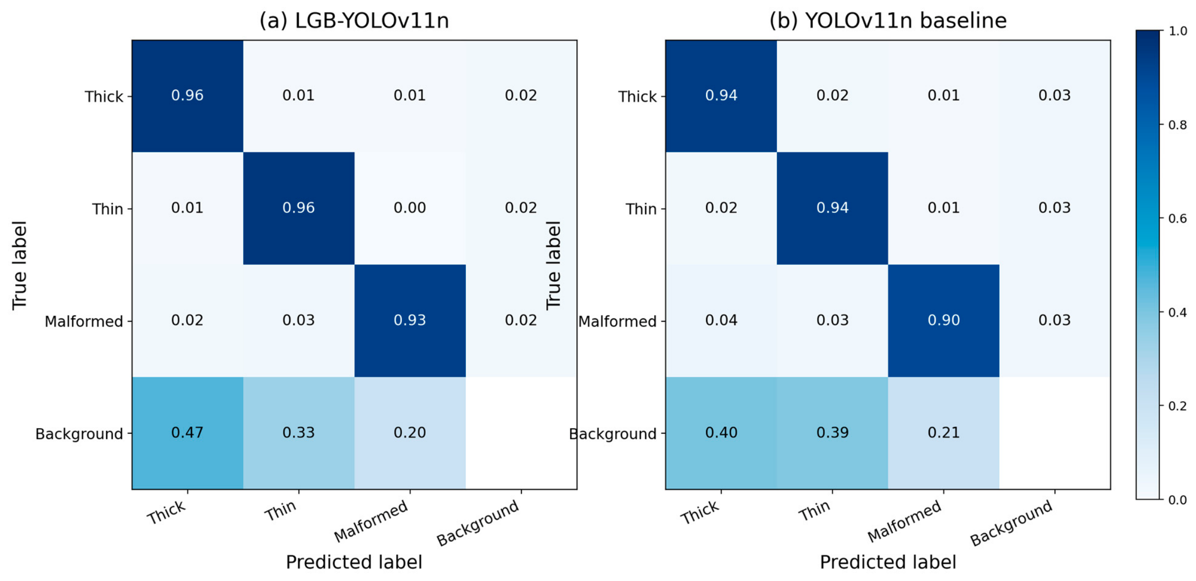
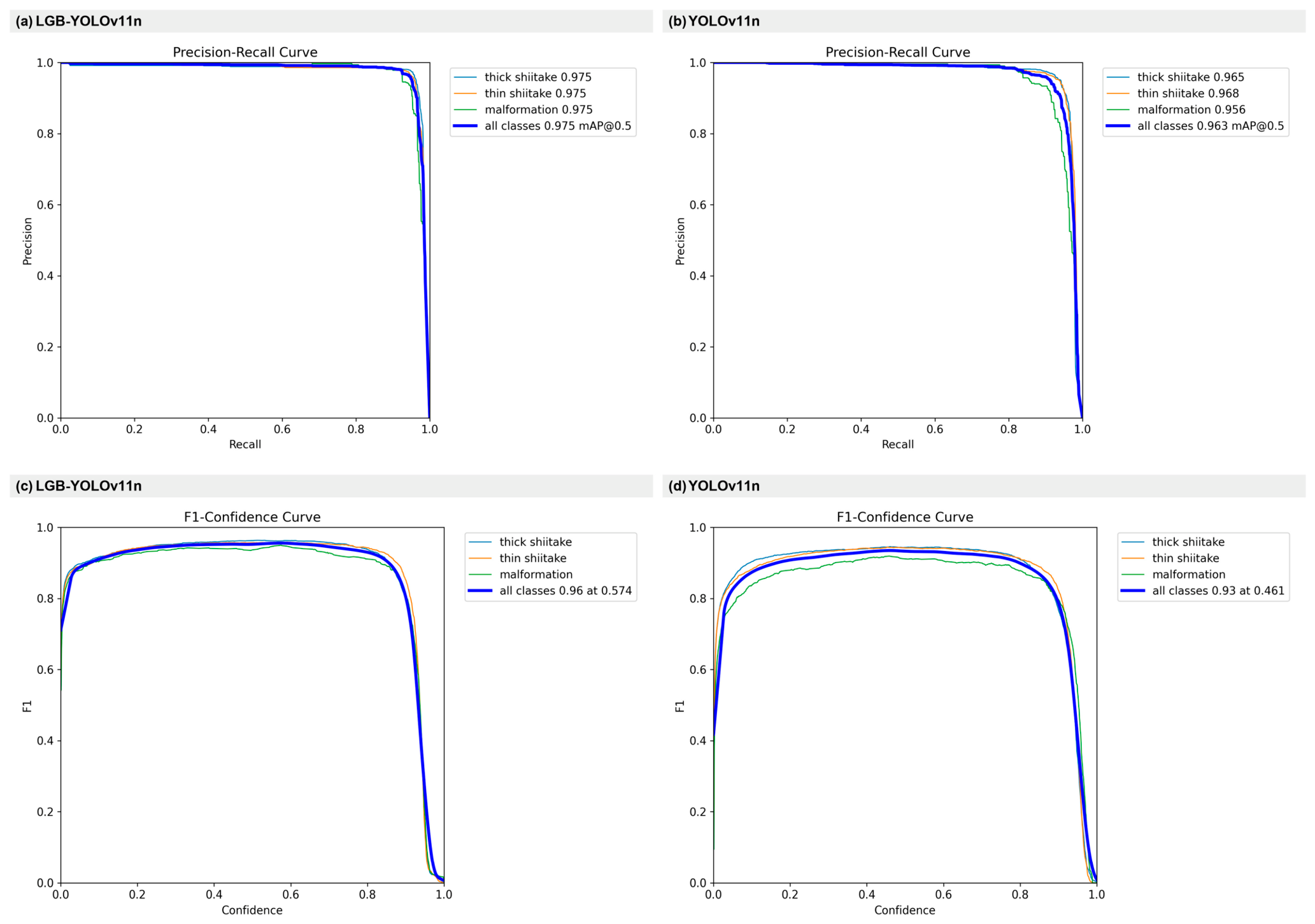
To analyze performance across shiitake appearance categories, class-wise AP@0.5 was compared for thick, thin, and malformed shiitake on the held-out test set. Normalized confusion matrices, precision-recall (PR) curves, and F1-confidence curves were further used to examine class confusion and confidence-threshold behaviour.

Table 13. Class-wise AP@0.5 comparison of the two models on the held-out test set.

Class	LGB-YOLOv11n AP@0.5 (%)	YOLOv11n Baseline AP@0.5 (%)	Gain (Percentage Points)
Thick shiitake	97.50	96.50	1.00
Thin shiitake	97.50	96.80	0.70
Malformed shiitake	97.50	95.60	1.90

Note: Class-wise AP@0.5 values are reported to two decimal places according to the legends in Figure 12; exact all-class results are reported in Table 8.

summarizes the class-wise AP@0.5 results of the two models, Figure 11 presents the normalized confusion matrices, and Figure 12 shows the PR and F1-confidence curves. Table 8 remains the primary unified numerical comparison across all evaluated detectors.

As shown in Table 13, LGB-YOLOv11n achieved an AP@0.5 of 97.50% for thick, thin, and malformed shiitake on the held-out test set, compared with 96.50%, 96.80%, and 95.60% for YOLOv11n, corresponding to gains of 1.00, 0.70, and 1.90 percentage points. The all-class mAP@0.5 values were 97.51% and 96.30% for LGB-YOLOv11n and YOLOv11n, respectively.

In Figure 11, the main-diagonal values for thick, thin, and malformed shiitake were 0.96, 0.96, and 0.93 for LGB-YOLOv11n, compared with 0.94, 0.94, and 0.90 for YOLOv11n. With true classes presented by row and predicted classes by column, the proportions of true foreground instances assigned to the background column were 0.02 for each of the three classes with LGB-YOLOv11n and 0.03 with the baseline at the evaluated threshold.

To further examine detection behaviour across recall levels and confidence thresholds, Figure 12 compares the PR and F1-confidence curves of the two models on the held-out test set.

As shown in Figure 12, the AP@0.5 values of LGB-YOLOv11n were 0.975 for thick, thin, and malformed shiitake, compared with 0.965, 0.968, and 0.956 for the YOLOv11n baseline. The all-class mAP@0.5 values were 0.975 and 0.963, consistent with the exact results reported in Table 8. The overall peak F1 values were 0.96 at a confidence threshold of 0.574 for LGB-YOLOv11n and 0.93 at 0.461 for the baseline.

3.9. Edge-Side Deployment Experiment

To evaluate edge-side deployability, the trained models were exported to an Open Neural Network Exchange (ONNX) format and further converted into TensorRT 16-bit floating-point (FP16) engines for inference testing on an NVIDIA Jetson Orin NX 16GB platform. All compared models used identical TensorRT build settings and test scripts, with a fixed input size of 640 × 640, a batch size of 1, and DLA disabled. The platform operated in MAXN 25 W mode, and the graphical interface and unnecessary background processes were disabled before testing. Each model was warmed up for 100 iterations, after which the mean and standard deviation over 1000 inference runs were calculated. System memory usage and power consumption were recorded using tegrastats.

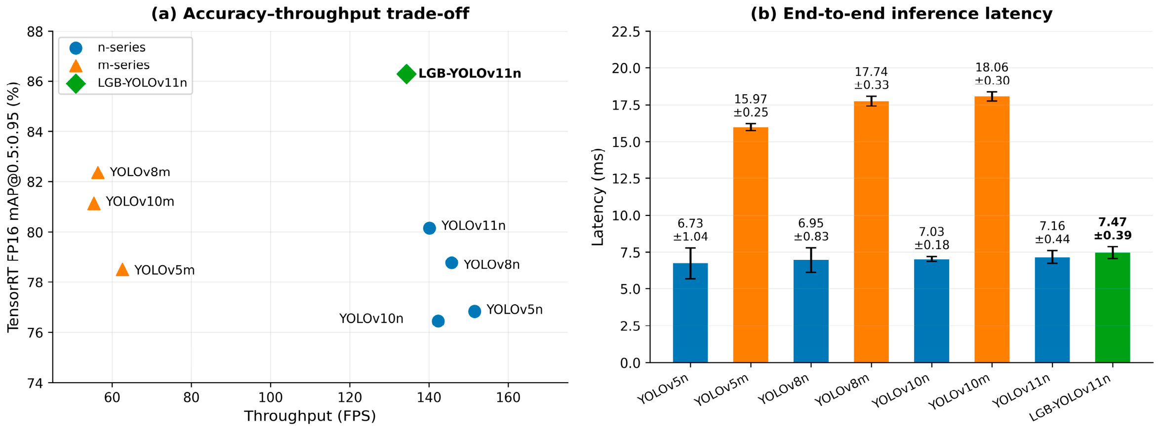
LGB-YOLOv11n achieved an end-to-end inference pipeline latency of 7.47 ± 0.39 ms on the Jetson Orin NX TensorRT FP16 backend, corresponding to 134.3 ± 6.73 FPS. The measured pipeline includes image pre-processing, TensorRT inference, and NMS/post-processing. The mean platform power draw was 18.56 ± 0.77 W, and the energy efficiency was 7.24 FPS/W. YOLOv11n achieved 7.16 ± 0.44 ms and 140.1 ± 7.87 FPS, with a mean power draw of 18.92 ± 1.28 W. The corresponding TensorRT-evaluated mAP@0.5:0.95 values were 86.29% and 80.15%, respectively.

Table 14. Accuracy and edge-side deployment performance comparison of different models on Jetson Orin NX.

Model	mAP@0.5 (%)	mAP@0.5:0.95 (%)	Latency (ms)	FPS	Power (W)	Engine (MB)
YOLOv5n	91.37	76.83	6.73 ± 1.04	151.5 ± 19.07	17.60 ± 1.61	7.40
YOLOv5m	93.18	78.51	15.97 ± 0.25	62.6 ± 0.98	28.77 ± 0.69	50.40
YOLOv8n	92.61	78.78	6.95 ± 0.83	145.7 ± 14.77	18.17 ± 1.40	8.10
YOLOv8m	95.52	82.36	17.74 ± 0.33	56.4 ± 1.05	29.90 ± 0.96	51.90
YOLOv10n	90.54	76.45	7.03 ± 0.18	142.3 ± 3.50	19.04 ± 0.79	6.30
YOLOv10m	94.13	81.13	18.06 ± 0.30	55.4 ± 0.90	29.19 ± 1.15	31.90
YOLOv11n	95.84	80.15	7.16 ± 0.44	140.1 ± 7.87	18.92 ± 1.28	7.60
LGB-YOLOv11n	97.42	86.29	7.47 ± 0.39	134.3 ± 6.73	18.56 ± 0.77	7.40

Note: The mAP values in Table 14 were obtained by reevaluating the TensorRT FP16 engines on the held-out test set, whereas those in Table 8 were obtained from the PyTorch models on the same held-out test set. The small differences are attributable to inference-backend conversion and FP16 numerical precision; Table 8 is retained as the principal accuracy comparison. Reported latency includes image pre-processing, TensorRT FP16 inference, and NMS/post-processing. FPS is derived from the same pipeline timing measurement. FPS, frames per second; FP16, 16-bit floating-point precision.

reports the complete deployment results, including accuracy, end-to-end inference pipeline latency, throughput, power draw, and engine size. Figure 13 presents the relationship between throughput and TensorRT-evaluated mAP@0.5:0.95 and the mean pipeline latency. All models were evaluated using the same TensorRT build settings, preprocessing procedure, NMS implementation, input size, power mode, and hardware state.

Across the TensorRT deployment results, the conventional nano-series detectors (YOLOv5n, YOLOv8n, YOLOv10n, and YOLOv11n) formed a low-latency, high-throughput regime, with mean latencies of 6.73–7.16 ms, throughputs of 140.1–151.5 FPS, and mAP@0.5:0.95 values of 76.45–80.15%. Their corresponding medium variants increased mAP@0.5:0.95 to 78.51–82.36%, but latency rose to 15.97–18.06 ms and throughput decreased to 55.4–62.6 FPS, together with higher power draw and substantially larger TensorRT engines. LGB-YOLOv11n achieved the highest TensorRT-evaluated mAP@0.5:0.95 of 86.29% while retaining an end-to-end latency of 7.47 ms, 134.3 FPS throughput, 18.56 W mean power draw, and a 7.40 MB engine. Relative to YOLOv11n, this corresponds to a 6.14-percentage-point increase in mAP@0.5:0.95 with a 0.31 ms latency increase and a 5.8 FPS throughput decrease, while power draw and engine size are slightly reduced.

3.10. Error Analysis on Illustrative Complex Scenes

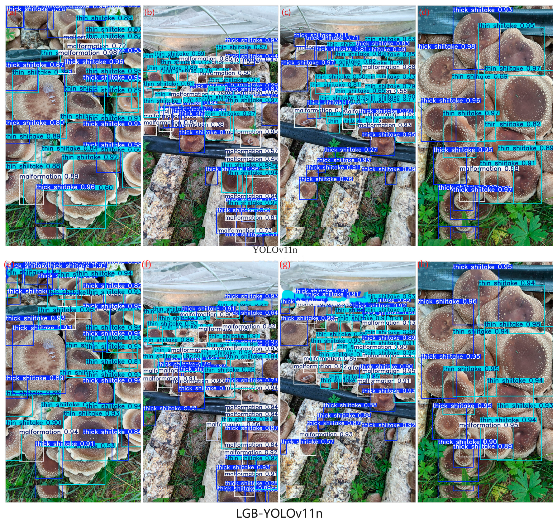
Error inspection identified four recurrent conditions in the held-out test images: (1) thick–thin confusion in visually transitional samples; (2) low-confidence or missed detections for small targets; (3) missed, overlapping, or uncertain detections under severe occlusion and adhesion; and (4) occasional false positives associated with cultivation logs, plastic film, grass, local shadows, and irregular background textures. Malformed shiitake also showed errors in cases of extreme deformation, severe damage, and partial visibility.

Figure 14 compares the two models on four illustrative complex samples using identical visualization settings. The examples include dense aggregation and scale variation (Figure 14a,e), small targets and partial occlusion (Figure 14b,f), severe adhesion and cluttered backgrounds (Figure 14c,g), and local overlap with incomplete target boundaries (Figure 14d,h). The figure is provided as a qualitative complement to the quantitative held-out test results.

4. Discussion

The engineering relevance of this study lies in coordinating feature representation, model compression, and multi-scale fusion with the requirements of forest-understory appearance pre-grading. The position-specific ablations show that different feature levels respond differently to contextual enhancement and compression. LSA produced its strongest validation result when jointly deployed at the P4/16 backbone level and the high-resolution P3 detection branch, whereas extending it to all detection branches did not further improve the selected metric. Similarly, Ghost compression was better tolerated in the P4/P5 branches than in P3. These observations support treating module placement as a task-dependent design variable rather than assuming that a useful module should be uniformly inserted throughout the feature hierarchy.

The comparative results in Table 8 reveal several trends beyond the ranking of individual models. First, moving from nano/tiny variants to medium variants generally increases Precision, Recall, and mAP, but the computational cost rises disproportionately. For example, YOLOv8m increases mAP@0.5:0.95 from 78.87% for YOLOv8n to 82.47%, while the parameter count rises from 2.69 M to 23.22 M and FLOPs from 6.90 G to 67.80 G. A similar pattern is observed for YOLOv10n/m. Second, minimizing parameter count alone is insufficient: YOLOv9t uses only 2.00 M parameters but reaches 79.57% mAP@0.5:0.95, whereas LGB-YOLOv11n uses 2.39 M parameters and reaches 86.62%. Third, adding generic attention to YOLOv11n improves some metrics only modestly: SE and CBAM yield 81.33% and 82.13% mAP@0.5:0.95, respectively, compared with 86.62% for the position-specific LGB configuration. LGB-YOLOv11n also provides the highest Precision (97.45%), Recall (93.85%), mAP@0.5 (97.51%), and mAP@0.5:0.95 (86.62%) among the evaluated models while remaining below the YOLOv11n baseline in parameters, FLOPs, and weight-file size. The gain over YOLOv11n is substantially larger for mAP@0.5:0.95 (+5.62 percentage points) than for mAP@0.5 (+1.21 points), which is consistent with improved localization quality across stricter IoU thresholds rather than only more permissive IoU = 0.5 detection. Taken together, the table indicates that the principal benefit is not simply a larger or more heavily attended network, but a more favorable allocation of representation capacity under a compact computational budget.

Cross-batch, cross-domain, and training-sensitivity analyses address complementary aspects of reliability. Leave-one-acquisition-date-out validation yielded gains over YOLOv11n in all three folds, indicating that the improvement was retained when an acquisition date was excluded from training. On the 222-image external set, the newly added single-class evaluation showed that LGB-YOLOv11n achieved 87.16% Precision, 83.47% Recall, 89.52% AP@0.5, and 63.71% AP@0.5:0.95, exceeding YOLOv11n by 2.84, 3.32, 2.79, and 3.87 percentage points, respectively. Because the external images differ in source, scene composition, viewpoint, and illumination and were evaluated without fine-tuning, this experiment provides a more direct quantitative test of source–domain transfer than the previous qualitative comparison alone. The added convergence/regularization sensitivity experiment yielded only marginal increases over the 86.40% reference result: 86.52% after extending training to 400 epochs and 86.47% with stronger weight decay (0.001). The small gains from longer training and stronger regularization indicate that the 300-epoch reference configuration was already near a stable validation-performance plateau under the evaluated settings. These experiments do not establish global hyperparameter optimality, but they provide evidence that the reported configuration is not simply a consequence of an obviously under-trained reference setting. The training-set-size learning curve provides a complementary check on data sufficiency. Validation mAP@0.5:0.95 rose from 81.72% at 40% of the training data to 83.91%, 85.34%, and 86.40% at 60%, 80%, and 100%, respectively. The successive gains of 2.19, 1.43, and 1.06 percentage points show diminishing returns as the available training set is approached. This trend suggests that the current training set provides a reasonably adequate scale for the evaluated configuration, while the remaining positive slope also indicates that further data collection may still yield additional improvement.

The class-wise results and error analysis also expose the present limitations. The thick and thin categories are operational appearance labels inferred from monocular RGB images rather than direct three-dimensional thickness measurements. Consequently, transitional samples with weak texture, edge-curling, shading, or cap-expansion cues can remain ambiguous. Small targets lose spatial detail after downsampling, while severe occlusion and adhesion reduce visible cap area and make instance separation difficult. Background structures such as cultivation logs, grass, plastic film, and local shadows can generate false positives. In addition, malformed shiitake are less frequent and display substantial intra-class variability. Future work should therefore incorporate independent expert scoring, quantitative inter-annotator agreement, and side-view, RGB-D, or multi-view information to relate appearance categories to measured cap traits.

The deployment comparison (the reviewer’s original Table 11; renumbered Table 14 after the newly added cross-domain, training-sensitivity, and training-set-size analyses) shows a clear separation between nano-series and medium-series operating regimes. The nano-series models run at approximately 134–152 FPS with mean latencies of 6.73–7.47 ms, power draw of about 17.6–19.0 W, and compact TensorRT engines of 6.3–8.1 MB, but their mAP@0.5:0.95 values remain between 76.45% and 80.15%. In contrast, the medium models improve some accuracy measures but require 15.97–18.06 ms, only 55.4–62.6 FPS, approximately 28.8–29.9 W, and substantially larger 31.9–51.9 MB engines. LGB-YOLOv11n remains within the nano-series end-to-end latency/power envelope while providing the highest TensorRT-evaluated mAP@0.5:0.95 (86.29%). Relative to YOLOv11n, it gains 6.14 percentage points in mAP@0.5:0.95 while latency increases by only 0.31 ms (7.16 to 7.47 ms) and throughput decreases by 5.8 FPS (approximately 4.1%); meanwhile, mean power draw decreases from 18.92 to 18.56 W and engine size from 7.60 to 7.40 MB. Relative to the faster YOLOv5n/YOLOv8n models, LGB-YOLOv11n accepts a moderate throughput reduction in exchange for markedly higher localization accuracy. The result should therefore be interpreted as an accuracy-oriented edge compromise rather than a claim of maximum FPS. The current deployment experiment remains model-level: the dataset was collected at a single cultivation site, and complete production-line integration with image triggering, conveyor timing, sorting hardware, actuator coordination, and continuous-operation testing has not yet been evaluated.

5. Conclusions

This study developed LGB-YOLOv11n for appearance-based pre-grading of the operational thick, thin, and malformed shiitake categories. The method combines LSA at the backbone P4/16 layer and the P3/8 detection branch, Ghost modules in the P4/16 and P5/32 detection branches, and BiFPN_WF at four neck fusion nodes. The selected configuration was determined through full-factorial and position-specific validation-set ablations.

On the held-out test set, LGB-YOLOv11n achieved mAP@0.5 and mAP@0.5:0.95 values of 97.51% and 86.62%, respectively, compared with 96.30% and 81.00% for YOLOv11n. The parameter count decreased from 2.59 M to 2.39 M, FLOPs from 6.40 G to 6.20 G, and weight-file size from 5.20 MB to 4.80 MB. Repeated random-seed experiments showed limited variation, and the three acquisition-date folds retained gains over the baseline. On the Jetson Orin NX, the model achieved real-time TensorRT FP16 inference at 134.3 FPS. Single-class cross-domain evaluation on the external image set yielded 89.52% AP@0.5 and 63.71% AP@0.5:0.95, compared with 86.73% and 59.84% for YOLOv11n, providing quantitative evidence in addition to the qualitative examples. The training-set-size learning curve increased from 81.72% mAP@0.5:0.95 at 40% of the training split to 86.40% at 100%, with progressively smaller gains, supporting the reasonable adequacy of the current training-set scale under the evaluated configuration.

Several current performance limitations should be emphasized. The appearance categories are inferred from monocular RGB images and therefore cannot directly encode three-dimensional cap thickness; transitional thick–thin samples with weak visual cues can remain ambiguous. Small mushrooms, severe occlusion or adhesion, and highly variable malformed targets remain the main sources of missed detections or class confusion, while cluttered cultivation logs, grass, plastic film, and local shadows can still cause false positives. The single-class external evaluation improves over the YOLOv11n baseline but reaches 63.71% AP@0.5:0.95, showing that cross-domain transfer is not yet complete under changes in source, viewpoint, illumination, and background composition. In addition, the self-built dataset was collected at a single cultivation site, and the Jetson experiment evaluates model-level inference rather than an integrated sorting line. Future work will therefore expand data collection across production sites, devices, dates, seasons, and cultivars; incorporate independent expert annotation and quantitative agreement analysis; relate visual categories to measured cap traits; evaluate side-view, depth, and multi-view information; and conduct integrated sorting trials to quantify end-to-end throughput and pre-grading consistency.