Prototyping a Compact Moisture Profiling Probe for Detecting and Zoning Hidden Subsurface Waterlogging

Abstract

Hidden waterlogging of subsurface soils may develop without clear external signs, while still deteriorating the hydro-physical state of foundation soils. This proof-of-concept study demonstrates a compact monitoring and interpretation workflow for identifying such zones through moisture profiling and subsequent engineering interpretation using the liquidity index (${\mathrm{I}}_{\mathrm{L}}$) for cohesive soils and the saturation ratio (${\mathrm{S}}_{\mathrm{r}}$) for non-cohesive soils. The developed prototype comprises a modular immersion probe, Arduino-based transmitter and receiver units, 433 MHz ASK wireless communication, and data logging. Using geotechnical survey data from a representative site in Astana, a baseline hydro-physical state and an intentionally constructed synthetic risk-waterlogging scenario were analyzed through vertical profiles and horizontal interpolation maps. Under the baseline state, moisture content varied mainly from about 6 to 23%, while most ${\mathrm{I}}_{\mathrm{L}}$ and ${\mathrm{S}}_{\mathrm{r}}$ values remained within the normal zone. In the synthetic scenario, the response was much stronger in cohesive soils, where ${\mathrm{I}}_{\mathrm{L}}$ increased from about −0.55 to 1.8, whereas ${\mathrm{S}}_{\mathrm{r}}$ in non-cohesive soils changed only slightly. The Welch’s t-test indicated significant scenario-related changes for ${\mathrm{I}}_{\mathrm{L}}$ (p-value of 1.095 × 10⁻¹⁹) but not for ${\mathrm{S}}_{\mathrm{r}}$ (p-value of 0.147). The results show the methodological potential of the proposed workflow for engineeringly interpretable zoning of hidden waterlogging; however, site-specific calibration, metrological characterization, and field validation are still required before practical deployment.

1. Introduction

In engineering geology and geotechnical engineering, waterlogging in built-up areas and building foundations is regarded as an adverse natural and anthropogenic process caused by changes in the area’s hydrogeological regime and disruption of the natural water balance [1]. The process of waterlogging manifests not only as a rise in the groundwater level but also as an increase in the moisture content of the foundation soil, leading to changes in its physical and mechanical properties, reduced bearing capacity, and the development of deformations in building foundations [2]. In today’s building construction and operation conditions, the phenomenon of hidden waterlogging is becoming particularly significant [3]. Unlike visible waterlogging, which is accompanied by a sustained rise in the groundwater level to dangerous levels or the emergence of water at the surface, hidden waterlogging develops without distinct external signs and, usually, is not detected during standard groundwater level monitoring [4,5]. At the same time, the worsening of the deformation properties of the foundation begins before the groundwater level reaches critical levels, which significantly complicates the timely identification of risks and the implementation of engineering measures [6].

When assessing the consequences of waterlogging, the actual condition of the foundation soil is of decisive importance. For cohesive soils (i.e., clays), it is characterized by the liquidity index, which reflects changes in consistency as moisture content increases [7], and for non-cohesive soils (i.e., sands) by the degree of saturation, which determines the operating conditions of the soil skeleton [8]. Changes in these parameters are directly linked to the development of foundation settlement and can serve as a sensitive indicator of the early stages of hidden waterlogging [9,10].

Current regulatory and design documents address waterlogging mainly through engineering protection, engineering–geological surveys, groundwater level assessment, and the impact of water saturation on soil properties [11,12,13,14,15,16]. However, practical diagnosis still relies mainly on groundwater-table depth, while moisture redistribution within the aeration zone and its effect on standard soil-state indicators are considered only indirectly [17,18]. Similarly, international geotechnical design practice emphasizes hydrogeological conditions, pore pressures, moisture content, and soil-property variability, but does not explicitly define hidden waterlogging as a separate diagnostic category [13,19]. This creates a methodological gap between hydrogeological observation and geotechnical interpretation of the actual soil state.

A review of existing studies [20,21] shows that waterlogging risk assessments are typically based on the results of engineering–geological surveys, episodic observations of groundwater levels, and computational forecasts. This approach is justified at the design stage; however, during building operation, it does not allow tracking dynamic changes in the soil massif’s moisture state, especially in the presence of local anthropogenic impacts that develop over time [2,22]. A separate area of research involves the use of geophysical and electrical methods to assess soil moisture and water saturation [23,24]. It has been established that the electrical properties of soil are sensitive to changes in volumetric moisture content ($\mathsf{\theta }$, %), but the nature of these changes varies significantly depending on the soil type, its density, and composition [25,26,27]. In most such studies, to assess the moisture state of the medium, the electrical resistance ($R$, Ω) is initially measured and then converted to the resistivity (${\mathsf{\rho }}_{\mathrm{e}}$, Ω·m) using a geometric factor that accounts for the design and arrangement of the electrodes [28]. Next, calibration tests are conducted to determine the relationship between volumetric moisture content and the resistivity “$\mathsf{\theta }-{\mathsf{\rho }}_{\mathrm{e}}$”. The nature of this relationship is determined by the soil type, its density, mineralogical composition, degree of mineralization, and the chemical properties of pore water, including the pH level, which affects ion mobility and the electrical conductivity of the soil medium [29,30,31]. In recent years, interest in sensor-based and wireless soil foundation monitoring systems has been growing [32,33]. However, existing solutions are characterized by high cost, a stationary nature, or insufficient spatial resolution with respect to depth [34,35,36]. Furthermore, the measured parameters are used in their raw form and are not converted into soil condition indicators, which hinders the practical application of the results when assessing the reliability of building and facility foundations.

Thus, despite recognition of the danger posed by hidden waterlogging, there are currently no methods for detecting its early stages based directly on the geotechnical properties that characterize the condition of the foundation soil. Meanwhile, in current standards [15,37,38,39], the condition of clay soils is defined by the liquidity index, and that of sandy soils by the degree of saturation, which reflects their consistency and moisture regime. However, regulatory documents do not establish a direct link between these standard soil conditions and the engineering classification of waterlogged zones. Therefore, this study proposes using standard soil condition indicators as a quantitative basis for delineating subsurface waterlogged zones. This is because an increase in moisture content is accompanied by a regular transition of clay soils from a solid state to a plastic state and then to a liquid state, and of sandy soils from a low-moisture state to a water-saturated state, reflecting the sequential stages of change in their moisture regime characteristic of the waterlogging process [40]. In this study, these thresholds are considered as indicators of the stages of hidden waterlogging and are interpreted in terms of identifying normal zones, risk zones, and waterlogged zones. Accordingly, this study tests the following working hypotheses: (i) depth-resolved moisture-related measurements can be converted into standard geotechnical state indicators that are more directly interpretable for foundation assessment than raw electrical or moisture values; and (ii) a synthetic deterioration of the hydro-physical state will produce a stronger zoning response in cohesive soils through liquidity index than in non-cohesive soils through saturation ratio under the examined site conditions. Thus, the objective of this study is to demonstrate, at the proof-of-concept level, a workflow for identifying potential hidden waterlogging zones by combining depth-resolved moisture profiling with standard geotechnical indicators: liquidity index for cohesive soils (clays) and the degree of water saturation (saturation ratio) for non-cohesive soils (sands). The study includes: (i) development of a compact modular probe prototype with Arduino-based 433 MHz ASK data transmission; (ii) demonstration of the transition from electrical resistivity or moisture-related measurements to hydro-physical indicators using published $\mathsf{\theta }-{\mathsf{\rho }}_{\mathrm{e}}$ relationships; and (iii) vertical and horizontal zoning of normal and synthetic risk-waterlogging states for a representative site in Astana.

2. Materials and Methods

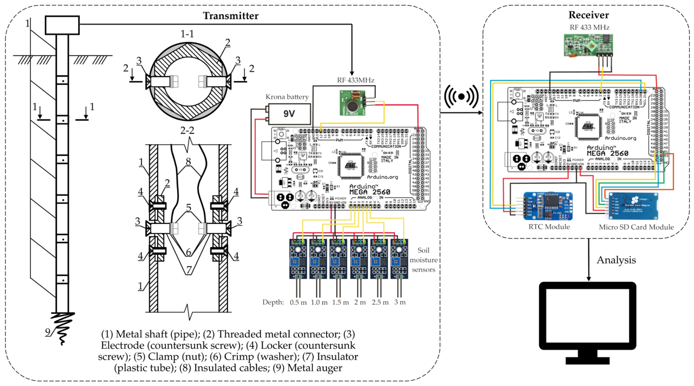
Figure 1 shows the architecture of a monitoring system for detecting hidden waterlogging of the subsurface, comprising an extendable immersion probe, a transmitter unit, and a receiver unit.

As shown in Figure 1, the immersion probe is designed as a modular metal shaft with an auger tip, allowing it to be buried in the ground with minor effort. The structure consists of 0.5 m long segments connected by threaded metal connectors. One sensor unit is installed on each added segment, so the number of measurement channels increases proportionally to the probe’s length. In the current configuration, with a length of 3.0 m, six channels are used, corresponding to depths of 0.5, 1, 1.5, 2, 2.5, and 3 m. The electrodes of each channel are led through the wall of the metal connector and come into contact with the surrounding soil, while their electrical connection to the transmitter unit is provided by insulated conductors laid inside the probe shaft. Thus, the system provides vertical profiling of soil moisture conditions with respect to depth. It should be noted that the fabricated probe configuration shown in this study has a current physical length of 3.0 m and therefore represents the hardware concept and data-acquisition principle. The subsequent analysis at 4.5 m and 9.5 m is based on geotechnical survey data and synthetic scenario modelling rather than on direct measurements by the current 3.0 m prototype. These deeper planes were used to demonstrate how the proposed interpretation approach may be applied after probe scaling or when combined with geotechnical investigation data.

The transmitter unit is built on the basis of an Arduino Mega 2560 (Arduino S.r.l., Strambino, Italy) and is designed to sequentially query measurement channels, convert signals into digital form, and transmit the results via a 433 MHz wireless radio channel. In the current implementation, data exchange relies on inexpensive 433 MHz RF transmitter/receiver modules with ASK modulation and the RH_ASK library; such modules are used to transmit short messages between two microcontrollers and require the correct pinout selection for the specific module during connection [41]. In the transmitter unit, the measurement channels are connected to the analog inputs of the Arduino Mega. For a six-level configuration, inputs A0–A5 are used. Each channel is sampled independently, after which the read analog value is converted to the volumetric moisture content using a calibration relationship between reference values for the conditionally dry and conditionally wet states. Next, the microcontroller forms a single data packet containing the packet number, the number of active channels, and the moisture values for all depths, and transmits it over the radio channel. The transmitter node in the circuit is powered by a 9 V battery connected to the VIN input of the Arduino board.

The receiver unit is also implemented on an Arduino Mega 2560 and handles data reception, time stamping, and archiving. The receiver’s radio module is connected to digital input D2, which is used by the RH_ASK library to receive packets. The DS3231 real-time clock (RTC) module, connected via the I²C interface, is used to record the date and time of measurements. For the Arduino Mega, the I²C lines are routed to the corresponding SDA and SCL pins on the board. Archiving is implemented via a microSD module connected via the SPI interface; for the Arduino Mega, the hardware SPI lines and SD chip selection are configured via the corresponding SPI pins, and the code uses the CS line = 53. After receiving a packet, the microcontroller checks its structure, adds a date and time stamp, and saves the results to a CSV file on the memory card, which enables subsequent processing on an external computer.

The software component of the system was developed in C/C++ for the Arduino platform using the Arduino IDE v. 2.3.7 (Qualcomm, Malmö, Sweden). The software implementation uses the RH_ASK library for radio data transmission, RTClib for working with the real-time module, Wire for communication via the I²C interface, as well as SPI and SD for writing data to a microSD memory card. The source code for the transmitter and receiver units is presented in Appendix A.1 and Appendix A.2, respectively.

In the present configuration, the prototype should be considered a concept demonstrator rather than a certified measuring instrument. The depth resolution is 0.5 m, corresponding to the spacing of the modular probe segments, and the current 3.0 m configuration includes six measurement channels. The Arduino Mega 2560 provides 10-bit analog-to-digital conversion, so the raw sensor response is recorded in the range of 0–1023 ADC units and then mapped in the software to a conditional 0–100% moisture scale using reference constants for dry and wet states. In the present prototype, these constants serve only for demonstrating signal conversion and data transmission; they were not obtained from standardized calibration tests on the local soils. Therefore, absolute measurement accuracy, resistivity measurement range, long-term signal stability, wireless transmission reliability under field interference, and durability under wet soil conditions were not yet quantified. These characteristics must be determined during the next stage of laboratory calibration and field validation.

In terms of scalability, the current architecture allows for direct extension of the probe length as long as the microcontroller’s analog inputs are sufficient. The Arduino Mega 2560 has 16 analog inputs, so without external expansion, the system can operate with a maximum of 16 channels, which, with a 0.5 m step, corresponds to a probe length of up to 8.0 m. If it is necessary to further increase the number of levels, external expansion devices must be used, such as analog multiplexers or additional ADCs. Furthermore, as the number of channels increases, it is undesirable to use long text strings for radio transmission, since ASK communication at 433 MHz is better suited for short packets, and the communication range is significantly affected by supply voltage, radio interference, and the antenna. Therefore, for a scalable system, it is advisable to use a compact binary packet, as shown in the sketches of Appendix A.1 and Appendix A.2. In the future, if reliable reception is required at distances significantly greater than 100 m, as well as with further development of the system toward a distributed multi-channel network, a transition to LoRa modules might be considered [42]; however, this is not implemented in the current version.

The present solution proposes using the data set collected in the receiver to subsequently interpret the hydro-physical state of the subsurface at each depth using the liquidity index (${\mathrm{I}}_{\mathrm{L}}$) for clay soils and the saturation ratio (${\mathrm{S}}_{\mathrm{r}}$) for sandy soils, based on the conditions in

Table 1. Classification of soil state (adopted from [15]).

Soil Type	Normal State	Risk State	Waterlogging State
Clays	${\mathrm{I}}_{\mathrm{L}}<0$	$0<{\mathrm{I}}_{\mathrm{L}}\le 1$	${\mathrm{I}}_{\mathrm{L}}>1$
Sands	$0<{\mathrm{S}}_{\mathrm{r}}\le 0.5$	$0.5<{\mathrm{S}}_{\mathrm{r}}\le 0.8$	$0.8<{\mathrm{S}}_{\mathrm{r}}\le 1$

according to [15], provided that there is a calibrated relationship between the measured electrical resistivity (${\mathsf{\rho }}_{\mathrm{e}}$) and volumetric moisture content ($\mathsf{\theta }$), i.e., “$\mathsf{\theta }-{\mathsf{\rho }}_{\mathrm{e}}$”.

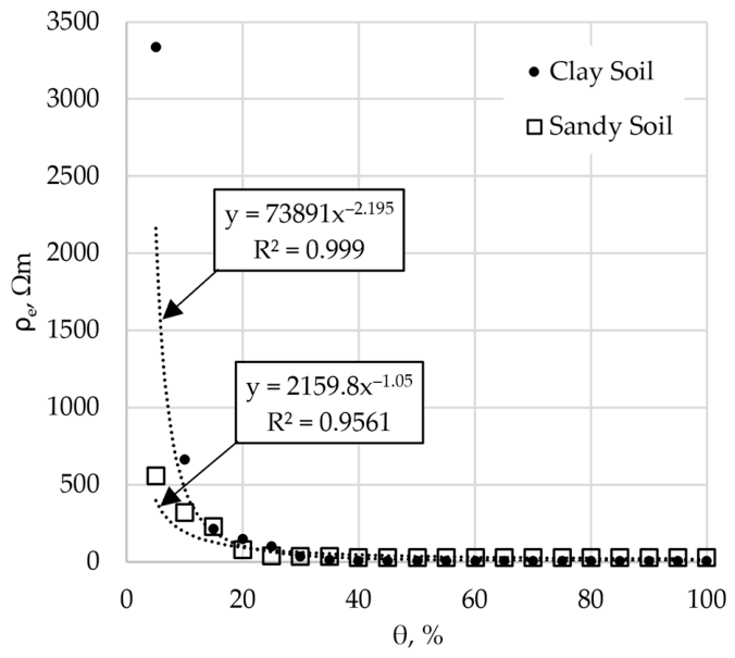
As part of this proof-of-concept study, no site-specific laboratory calibration tests were conducted to determine the relationship “$\mathsf{\theta }-{\mathsf{\rho }}_{\mathrm{e}}$” for the soils from the selected site. Therefore, the relationships for clayey and sandy soils reported in [26] were used only to illustrate the proposed computational workflow (Figure 2). This choice allows the sequence from electrical resistivity to moisture estimation and then to IL or Sr zoning to be demonstrated; however, it does not eliminate calibration uncertainty. Because $\mathsf{\theta }-{\mathsf{\rho }}_{\mathrm{e}}$ relationships are affected by soil type, density, mineralogical composition, pore-water chemistry, and electrode configuration, the resulting values should be interpreted as methodological estimates rather than validated field measurements for the selected site.

As shown in Figure 2, the $\mathsf{\theta }-{\mathsf{\rho }}_{\mathrm{e}}$ relationships for clayey and sandy soils are characterized by relatively high values of the coefficient of determination (R²) of 0.999 and 0.9561, respectively, indicating their suitability for use in our workflow when expressing the following equations [26]:

$${\mathsf{\rho }}_{\mathrm{e},\mathrm{c}}=73891·{\mathsf{\theta }}^{-2.195},\mathrm{or} {\mathsf{\theta }}_{\mathrm{c}}={\left({\displaystyle \frac{73891}{{\mathsf{\rho }}_{\mathrm{e},\mathrm{c}}}}\right)}^{{\displaystyle \frac{1}{2.195}}},$$

(1)

$${\mathsf{\rho }}_{\mathrm{e},\mathrm{s}}=2159.8·{\mathsf{\theta }}^{-1.05},\mathrm{or} {\mathsf{\theta }}_{\mathrm{s}}={\left({\displaystyle \frac{2159.8}{{\mathsf{\rho }}_{\mathrm{e},\mathrm{s}}}}\right)}^{{\displaystyle \frac{1}{1.05}}},$$

(2)

where ${\mathsf{\theta }}_{\mathrm{c}}$ and ${\mathsf{\theta }}_{\mathrm{s}}$—the volumetric moisture contents of clay and sand, respectively, %; ${\mathsf{\rho }}_{\mathrm{e},\mathrm{c}}$ and ${\mathsf{\rho }}_{\mathrm{e},\mathrm{s}}$—the electrical resistivities of clay and sand, respectively, Ω·m.

Equations (1) and (2) were used to obtain synthetic values of ${\mathsf{\rho }}_{\mathrm{e}}$ and to calculate $\mathsf{\theta }$, as well as to subsequently outline scenarios of the soil’s hydro-physical state at specified depths by visualizing the interpolated values of ${\mathrm{I}}_{\mathrm{L}}$ and ${\mathrm{S}}_{\mathrm{r}}$. The values of ${\mathrm{I}}_{\mathrm{L}}$ and ${\mathrm{S}}_{\mathrm{r}}$ can be calculated using established standard relationships. Some of these relationships are specified in the soil classification standard [15]:

$${\mathrm{I}}_{\mathrm{L}}={\displaystyle \frac{{\mathsf{\theta }}_{\mathrm{c}}-{\mathrm{W}}_{\mathrm{p}}}{{\mathrm{W}}_{\mathrm{L}}-{\mathrm{W}}_{\mathrm{p}}}}$$

(3)

$${\mathrm{S}}_{\mathrm{r}}={\displaystyle \frac{{\mathsf{\theta }}_{\mathrm{s}}·{\mathsf{\rho }}_{\mathrm{s}}}{\mathrm{e}·{\mathsf{\rho }}_{\mathrm{w}}}}$$

(4)

where ${\mathrm{W}}_{\mathrm{p}}$—plastic limit, %; ${\mathrm{W}}_{\mathrm{L}}$—liquid limit, %; ${\mathsf{\rho }}_{\mathrm{s}}$—density of solid particles, g/cm³; ${\mathsf{\rho }}_{\mathrm{w}}$—density of water (≈1.0 g/cm³); and $\mathrm{e}$—void ratio.

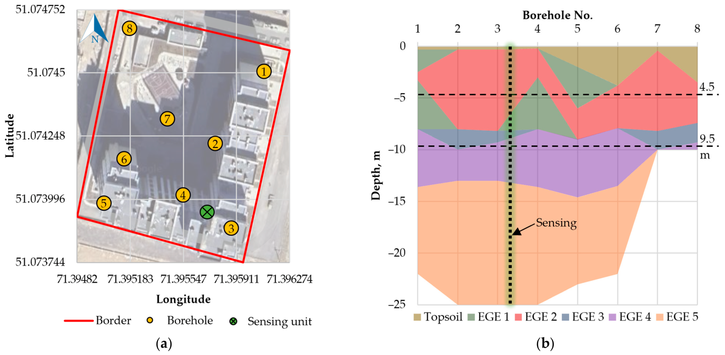
The parameters ${\mathrm{W}}_{\mathrm{p}}$, ${\mathrm{W}}_{\mathrm{L}}$, ${\mathsf{\rho }}_{\mathrm{s}}$, and $\mathrm{e}$ in Equations (3) and (4) vary from site to site and were therefore taken from the available geotechnical survey data for the selected representative site or from standard soil-property determinations [39,43,44,45] reported in the survey documentation [46]. The site (Figure 3) was selected as a representative engineering case because it is located in Astana (Kazakhstan), where subsiding loess and loess-like soils are relevant to hidden waterlogging problems, and because the available borehole data include the soil-type differentiation and hydro-physical parameters required for calculating ${\mathrm{I}}_{\mathrm{L}}$ and ${\mathrm{S}}_{\mathrm{r}}$. Thus, the site is used not as a fully validated field-monitoring test area, but as a realistic geotechnical basis for demonstrating the proposed interpretation workflow.

As shown in Figure 3a, eight boreholes were drilled at the site (with latitude and longitude geographical coordinates), the samples from which were used to determine the main properties of the soil profile (

Table A1. Data from geotechnical surveys at the construction site in Astana, Kazakhstan [46].

EGE and Consistency	Borehole No.	Sampling Depth, m	$\mathsf{\theta }$, %	${\mathbf{W}}_{\mathbf{p}}$, %	${\mathbf{W}}_{\mathbf{L}}$, %	${\mathsf{\rho }}_{\mathbf{s}}$, g/cm3	$\mathbf{e}$	${\mathbf{I}}_{\mathbf{L}}$	${\mathbf{S}}_{\mathbf{r}}$
EGE 1 Light brown sandy loam with a stiff and plastic consistency	1	1.3	6.23	13.70	19.70	2.70	0.500	−1.24	-
	1	7.2	23.05	17.10	23.50	2.70	0.698	0.93	-
	4	3.2	14.32	14.60	21.60	2.70	0.508	−0.04	-
	4	5.3	13.72	15.10	22.00	2.70	0.579	−0.20	-
	5	2.5	8.88	13.70	18.90	2.70	0.525	−0.93	-
	5	3.7	13.51	17.00	23.90	2.70	0.492	−0.51	-
EGE 2 Light brown loam with a stiff to stiff-plastic consistency	1	2.7	11.15	15.30	23.00	2.71	0.473	−0.54	-
	3	2.2	13.23	15.20	22.80	2.71	0.566	−0.26	-
	3	3.6	12.65	15.40	23.20	2.71	0.497	−0.35	-
	3	6.5	22.80	19.80	27.80	2.71	0.673	0.38	-
	4	1.8	12.01	15.10	23.20	2.71	0.514	−0.38	-
	5	7.0	22.49	22.10	33.20	2.72	0.700	0.04	-
	6	6.5	21.34	19.00	27.80	2.71	0.663	0.27	-
	7	2.0	10.57	14.60	23.00	2.71	0.397	−0.48	-
	7	4.5	12.61	15.00	23.30	2.71	0.549	−0.29	-
	7	6.7	23.02	21.80	32.90	2.72	0.711	0.11	-
EGE 3 Coarse sand with layers of sand of varying grain sizes	2	10.0	15.00	-	-	2.65	0.6	-	0.6
	7	9.7	14.62	-	-	2.65	0.6	-	0.6
EGE 4 Gravelly sand with layers of gravel	1	13.0	6.72	-	-	2.65	0.6	-	0.5
	3	11.5	11.26	-	-	2.65	0.6	-	0.5
	4	9.5	12.60	-	-	2.65	0.6	-	0.5
	5	9.0	12.26	-	-	2.65	0.6	-	0.5
	5	12.5	8.04	-	-	2.65	0.6	-	0.5
	6	11.0	6.45	-	-	2.65	0.6	-	0.5
	8	9.5	15.07	-	-	2.65	0.6	-	0.5
EGE 5 White, gray, red, and yellow loam with a stiff consistency	1	16.5	12.39	17.80	27.90	2.72	0.629	−0.54	-
	1	21.3	9.10	16.90	23.70	2.70	0.639	−1.15	-
	2	15.0	13.50	19.80	32.20	2.72	0.609	−0.51	-
	2	19.0	15.41	20.00	33.60	2.73	0.417	−0.34	-
	3	14.8	14.15	19.60	30.00	2.72	0.489	−0.52	-
	3	16.0	13.12	17.90	29.10	2.72	0.648	−0.43	-
	3	23.0	11.73	24.70	34.10	2.72	0.462	−1.38	-
	4	15.2	12.75	19.30	27.40	2.71	0.617	−0.81	-
	4	19.1	10.40	16.90	27.10	2.72	0.635	−0.64	-
	4	23.0	11.13	24.80	34.40	2.72	0.462	−1.42	-
	5	14.0	15.25	19.10	29.00	2.72	0.552	−0.39	-
	5	18.0	10.87	16.20	22.80	2.70	0.495	−0.81	-
	5	24.8	7.81	17.80	25.30	2.71	0.432	−1.33	-
	6	15.0	12.58	18.40	29.60	2.72	0.478	−0.52	-
	6	22.0	13.44	24.00	33.20	2.72	0.449	−1.15	-

), which consists of topsoil and five engineering–geological elements (EGE), as shown in Figure 3b [46]: EGE 1, 2, and 5 are predominantly represented by clays; EGE 3 and 4 are predominantly represented by sands. Figure 3b also shows two cutting planes defined at depths of 4.5 and 9.5 m. These depths were selected because they intersect different hydro-geotechnical parts of the profile: the 4.5 m plane crosses the upper cohesive loess and loam strata represented mainly by EGE 1 and EGE 2, whereas the 9.5 m plane crosses the deeper sandy strata represented mainly by EGE 3 and EGE 4. Thus, the two planes allow the proposed zoning workflow to be demonstrated separately for cohesive and non-cohesive soil conditions. In urban built-up areas, hydro-physical changes in the upper plane (4.5 m) may be caused by infiltration of atmospheric precipitation and leaks from utility lines, while in the lower plane (9.5 m), they may be caused by fluctuations in the groundwater table [47].

Table 2. Hydro-physical conditions of the soil massif of the study area.

EGE No.	Soil Type	Estimated by Equations (1) and (2) [26]	Average of Values from Table A1 [46]					Estimated by Equations (3) and (4) [15]
		${\mathsf{\rho }}_{\mathbf{e}}$, Ω·m	$\mathsf{\theta }$, %	${\mathbf{W}}_{\mathbf{p}}$, %	${\mathbf{W}}_{\mathbf{L}}$, %	${\mathsf{\rho }}_{\mathbf{s}}$, g/cm3	$\mathbf{e}$	${\mathbf{I}}_{\mathbf{L}}$	${\mathbf{S}}_{\mathbf{r}}$
1	Clays	252.821	13.285	15.2	21.6	2.7	0.5503	−0.299	-
2	Clays	163.859	16.187	17.33	26.02	2.712	0.5743	−0.132	-
3	Sands	127.447	14.81	-	-	2.65	0.6	-	0.654
4	Sands	185.814	10.342	-	-	2.65	0.6	-	0.457
5	Clays	302.521	12.242	19.546	29.293	2.712	0.5342	−0.749	-

presents a summary of the hydro-physical properties of the soils in the study area, broken down by EGE, measured and recorded at the moment of the survey.

Based on Table 2, the study area is interpreted as predominantly being in a normal hydro-physical state under the survey conditions, especially for the cohesive EGEs, where ${\mathrm{I}}_{\mathrm{L}}$ remains below 0. For the sandy EGEs, ${\mathrm{S}}_{\mathrm{r}}$ is also generally below the waterlogging threshold; however, EGE 3 has ${\mathrm{S}}_{\mathrm{r}}$ = 0.654, which falls within the risk interval according to Table 1. Therefore, the baseline condition should not be described as entirely normal in all layers, but rather as predominantly normal with a localized risk-level saturation state in EGE 3. To visualize this hydro-physical state, two-dimensional (2D) spatial interpolation of ${\mathrm{I}}_{\mathrm{L}}$ and ${\mathrm{S}}_{\mathrm{r}}$ on the above-defined cutting planes (4.5 and 9.5 m) was performed using the Ordinary Kriging method [48] with QGIS v. 3.34.3 (Open Source Geospatial Foundation, Beaverton, Oregon, OR, USA), which resulted in heatmaps of spatial distribution. To visualize another possible scenario, synthetic ${\mathsf{\rho }}_{\mathrm{e}}$ values were used to construct a risk-waterlogging case.

To assess variability in estimates, the coefficients of variation (CV) [49] were calculated and used only as descriptive measures of relative dispersion. To verify whether the imposed scenario produced statistically different ${\mathrm{I}}_{\mathrm{L}}$ and ${\mathrm{S}}_{\mathrm{r}}$ values compared with the baseline state, the profile-based data were analyzed using Welch’s two-sample unequal-variance t-test [50]. Welch’s test was selected because the two scenarios were not assumed to have equal variances. The test was applied to the corresponding sets of ${\mathrm{I}}_{\mathrm{L}}$ and ${\mathrm{S}}_{\mathrm{r}}$ values generated for the normal and synthetic risk-waterlogging scenarios; therefore, the resulting p-values characterize the statistical contrast between the constructed scenarios and should not be interpreted as validation against independent field measurements. The following null hypothesis (${\mathrm{H}}_0$) and alternative hypothesis (${\mathrm{H}}_1$) were set:

—

${\mathrm{H}}_0$: The values of ${\mathrm{I}}_{\mathrm{L}}$ and ${\mathrm{S}}_{\mathrm{r}}$ in scenarios do not differ statistically significantly; the observed changes are attributable to random variation.

—

${\mathrm{H}}_1$: The values of ${\mathrm{I}}_{\mathrm{L}}$ and ${\mathrm{S}}_{\mathrm{r}}$ in scenarios differ statistically significantly; the observed changes are associated with the risk and waterlogging scenario.

Additionally, to quantify the magnitude of changes, the descriptive statistics [51] were performed for the values from the interpolated ${\mathrm{I}}_{\mathrm{L}}$ and ${\mathrm{S}}_{\mathrm{r}}$ heatmaps for the observation depth (4.5 and 9.5 m) quantified from their raster images in tabular format.

3. Results

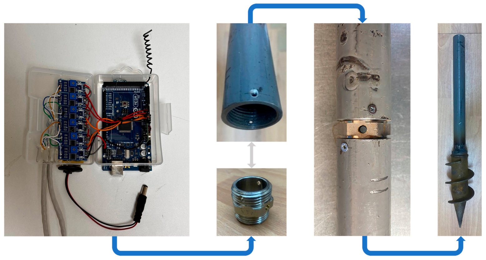
Figure 4 presents the fabricated proof-of-concept prototype of the proposed monitoring system, including the transmitter unit, the receiver unit, and the modular elements of the immersion probe.

As shown in Figure 4, the electronic part of the prototype was assembled in plastic housings for experimental testing and includes the microcontroller-based transmitter and receiver hardware required for data acquisition, wireless communication, and logging. The modular probe part is represented by segmented elements, including a 0.5 m metal shaft segment with internal threading, a threaded metal connector used to join adjacent shafts, and an assembled segment with electrode outlets and mechanical fastening details. The photographs confirm the feasibility of the proposed modular design and its hardware implementation. At the same time, the prototype should be regarded as an experimental assembly intended to validate the operating concept rather than as a finalized waterproofed field-ready system.

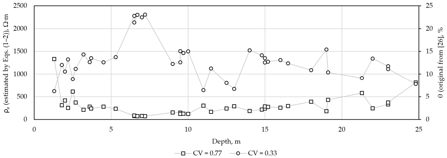
Figure 5 presents the initial hydro-physical background of the study area before introducing any synthetic risk or waterlogging scenario, by comparing the ${\mathsf{\rho }}_{\mathrm{e}}$ values estimated by Equations (1) and (2) with the original $\mathsf{\theta }$ from the geotechnical survey data. The moisture content varies within a relatively narrow range, mainly from about 6 to 23%, whereas the corresponding estimated resistivity spans a much wider interval, from roughly 60 to 2300 Ω·m. This contrast is also reflected by the coefficients of variation (CV), which are 0.33 for θ and 0.77 for ${\mathsf{\rho }}_{\mathrm{e}}$, showing that the electrical resistivity values are more dispersed than the corresponding moisture values in this dataset. Because CV is affected by scale, mean value, and the non-linear $\mathsf{\theta }-{\mathsf{\rho }}_{\mathrm{e}}$ transformation, this comparison is used only as a descriptive indicator of heterogeneity and is not treated as a statistical test of sensitivity. The subsequent zoning in is therefore based on ${\mathrm{I}}_{\mathrm{L}}$ and ${\mathrm{S}}_{\mathrm{r}}$ rather than on the CV comparison itself.

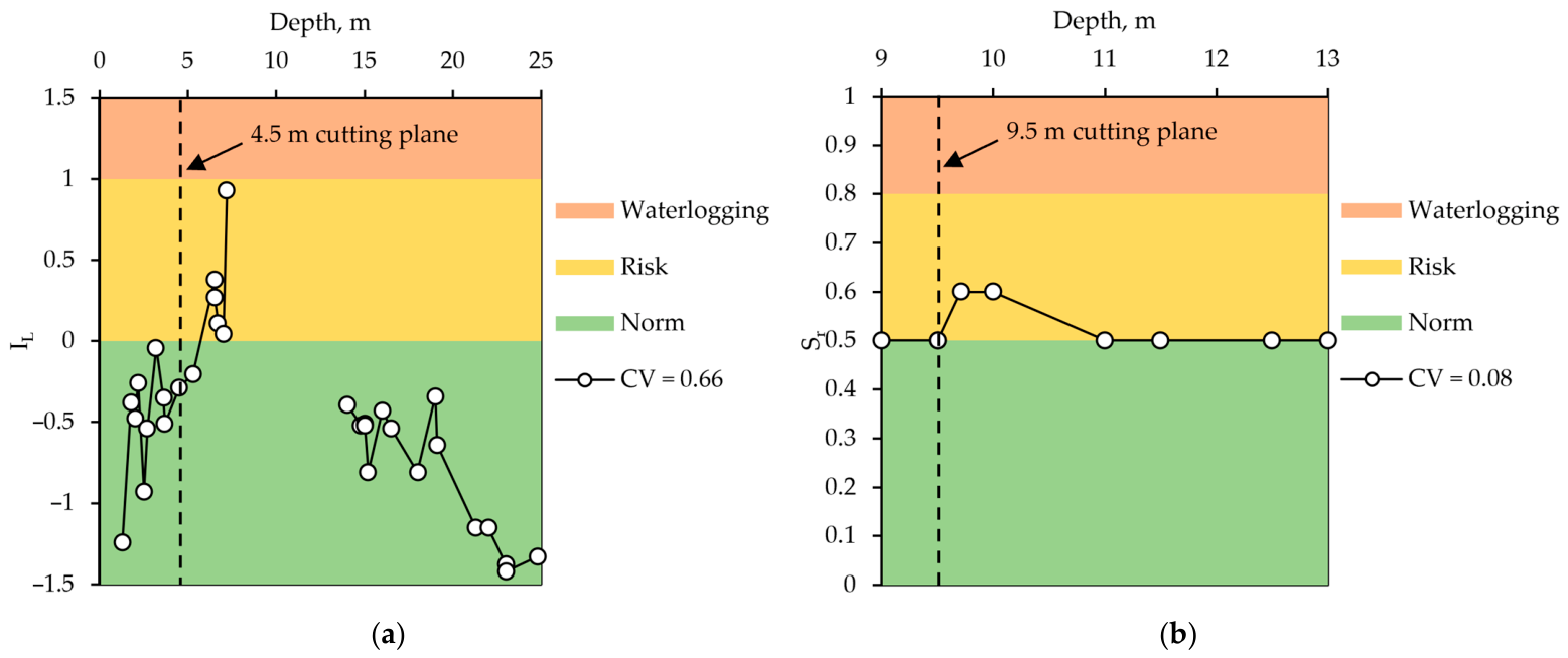
Figure 6 translates the baseline moisture-related estimates from Figure 5 into engineering zoning through the standard hydro-physical indicators ${\mathrm{I}}_{\mathrm{L}}$ and ${\mathrm{S}}_{\mathrm{r}}$. For the cohesive EGEs, most ${\mathrm{I}}_{\mathrm{L}}$ values remain within the normal zone (${\mathrm{I}}_{\mathrm{L}}$ < 0), generally from about −1.45 to −0.05, confirming a predominantly stable clay consistency profile; only a limited interval at depths of roughly 6.8–7.2 m rises into the risk zone, reaching about 0.93. For the non-cohesive EGEs, ${\mathrm{S}}_{\mathrm{r}}$ varies only from 0.49 to 0.60, with a very low CV = 0.08, indicating nearly uniform sandy conditions and only a local approach to the risk threshold. Thus, under the surveyed state, the vertical section is dominated by normal conditions, providing the reference case for comparison with the risk-waterlogging scenario and the horizontal zoning.

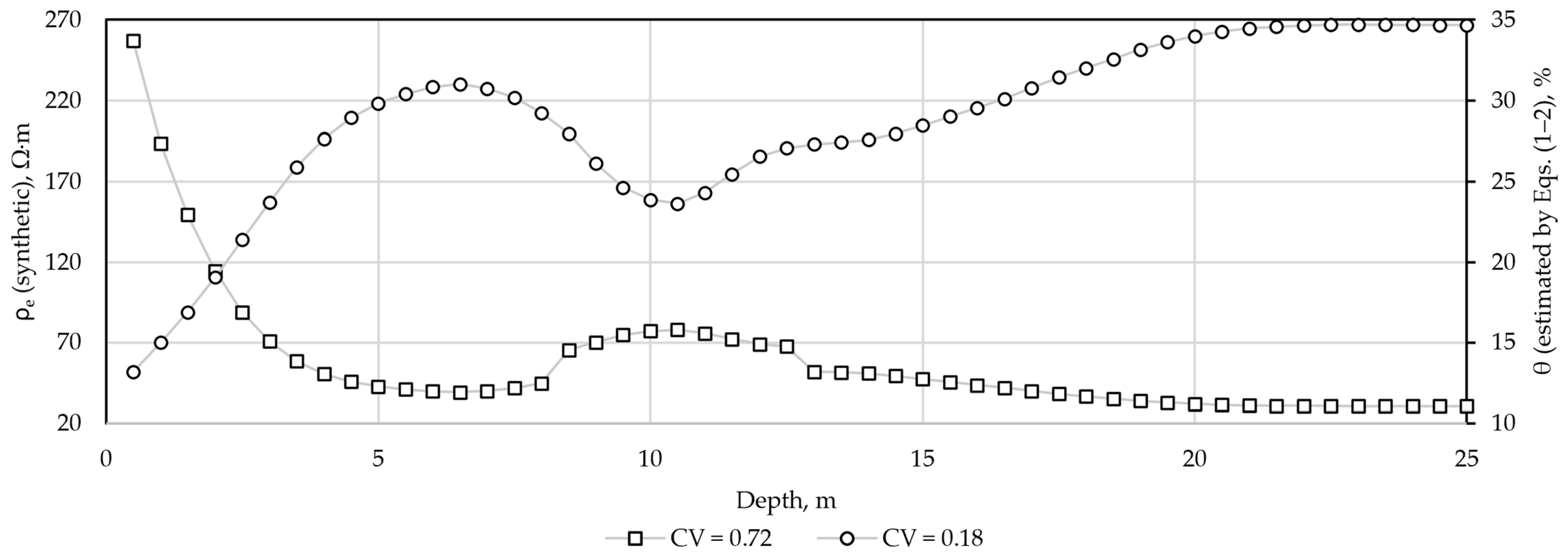
Figure 7 presents the alternative hydro-physical scenario introduced to demonstrate how the proposed workflow responds to a deterioration of the subsurface hydro-physical state. The synthetic ${\mathsf{\rho }}_{\mathrm{e}}$ values were intentionally selected to be lower than the baseline estimates because a decrease (Figure 5) in resistivity is generally associated with increasing moisture content. The selected range, mainly about 30–80 Ω⋅m after the upper interval, was not intended to reproduce a measured event at the site, but to remain within a physically plausible low-resistivity interval for wetter fine-grained and mixed subsurface conditions according to the adopted $\mathsf{\theta }-{\mathsf{\rho }}_{\mathrm{e}}$ relationships. No site-specific hydrogeological boundary conditions, leakage rates, or transient groundwater-flow model were imposed. Therefore, this scenario should be interpreted as a methodological stress test of the zoning procedure rather than as a prediction of actual field behavior. Compared with the baseline case, moisture variability becomes lower (CV = 0.18 versus 0.33), whereas resistivity remains highly variable (CV = 0.72); however, these CV values are interpreted descriptively and are not used alone to prove higher measurement sensitivity. This scenario forms the basis for the subsequent vertical and horizontal zoning of risk and waterlogging conditions.

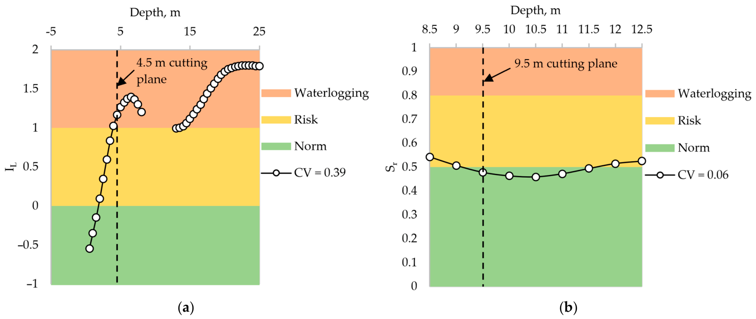
Figure 8 shows how the synthetic moisture-resistivity scenario from Figure 7 is translated into engineering zoning through ${\mathrm{I}}_{\mathrm{L}}$ and ${\mathrm{S}}_{\mathrm{r}}$. In the cohesive EGEs, the profile shifts markedly upward relative to the baseline case in Figure 6. Thus, ${\mathrm{I}}_{\mathrm{L}}$ rises from about −0.55 to 1.8, with only the shallowest interval remaining normal, while most of the section falls within the risk and waterlogging zones. At the 4.5 m cutting plane, ${\mathrm{I}}_{\mathrm{L}}$ is already about 1.15, i.e., within the waterlogging zone. In contrast, the non-cohesive EGEs remain comparatively stable, with ${\mathrm{S}}_{\mathrm{r}}$ varying only from about 0.46 to 0.54 (CV = 0.06). Thus, under this scenario, the main deterioration is concentrated in the cohesive strata, which is further examined in the horizontal zoning.

The Welch’s t-test confirms that the transition from the normal scenario to the risk-waterlogging scenario is statistically significant for the cohesive soils but not for the non-cohesive soils. Specifically, for the vertical zoning based on ${\mathrm{I}}_{\mathrm{L}}$, the obtained p-value of 1.095 × 10⁻¹⁹ is far below the conventional significance level of 0.05, so the null hypothesis is rejected, and the observed shift in clay consistency can be attributed to the imposed risk-waterlogging scenario rather than random variation. In contrast, for the zoning based on ${\mathrm{S}}_{\mathrm{r}}$, the p-value is 0.147, which exceeds 0.05. Therefore, the null hypothesis is not rejected, indicating that the changes in sandy soils are statistically insignificant within the examined scenario. This agrees with Figure 6 and Figure 8, where the strongest response is concentrated in the cohesive EGEs.

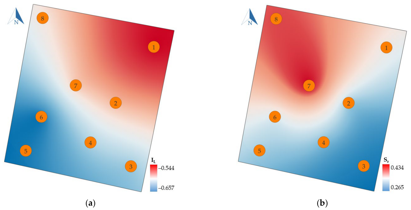
Figure 9 extends the normal vertical interpretation of Figure 6 into plan-view zoning at the two observation planes, showing that the surveyed subsurface remains within the normal hydro-physical state not only with depth, but also laterally across the site. At the 4.5 m cutting plane, the interpolated ${\mathrm{I}}_{\mathrm{L}}$ values vary only from about −0.657 to −0.544, i.e., entirely within the normal zone for cohesive soils, although a relative softening trend is visible toward the northeastern part of the site. At the 9.5 m cutting plane, the interpolated ${\mathrm{S}}_{\mathrm{r}}$ values range from about 0.265 to 0.434, also remaining below the risk threshold. Thus, Figure 9 provides the spatial reference background against which the altered zoning pattern in Figure 10 can be compared.

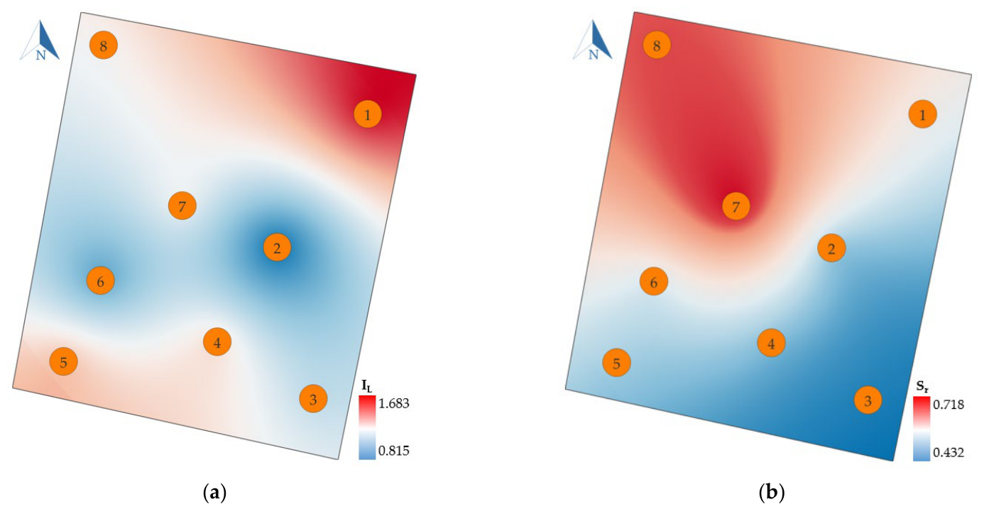
Figure 10 shows the plan-view manifestation of the imposed risk-waterlogging scenario and should be interpreted jointly with the baseline maps in Figure 9. At the 4.5 m cutting plane, the ${\mathrm{I}}_{\mathrm{L}}$-based pattern becomes markedly more heterogeneous, with the highest values concentrated in the northeastern part of the site near borehole 1 and a secondary elevated area toward borehole 5, while a comparatively less affected zone remains around the central part near boreholes 2 and 7. At the 9.5 m cutting plane, the ${\mathrm{S}}_{\mathrm{r}}$-based pattern also changes spatially, with the highest saturation developing in the northwestern to central part near boreholes 8 and 7, whereas the southeastern part near borehole 3 remains relatively less saturated. Thus, unlike Figure 9 and Figure 10 indicates that under the risk-waterlogging scenario, the subsurface state becomes laterally differentiated, and potential problem zones can be localized within specific sectors of the site rather than being distributed uniformly.

Table 3. Summary statistics.

Measure	Normal State (Figure 9)		Risk and Waterlogging State (Figure 10)
	${\mathbf{I}}_{\mathbf{L}}$ at 4.5 m	${\mathbf{S}}_{\mathbf{r}}$ at 9.5 m	${\mathbf{I}}_{\mathbf{L}}$ at 4.5 m	${\mathbf{S}}_{\mathbf{r}}$ at 9.5 m
Mean	−0.602949	0.336719	1.220882	0.550527
Standard error	0.000036	0.000055	0.00018	0.000093
Median	−0.602026	0.32685	1.212088	0.533395
Mode	−0.601027	0.298025	1.268756	0.663268
Standard deviation	0.031919	0.049187	0.160509	0.082677
Sample variance	0.001019	0.002419	0.025763	0.006835
Kurtosis	−1.112308	−1.367314	0.527888	−1.365405
Skewness	−0.000517	0.273767	0.549377	0.284009
Range	0.112872	0.169126	0.902515	0.285951
Minimum	−0.656914	0.26536	0.780456	0.431597
Maximum	−0.544042	0.434487	1.682971	0.717549
Sum	−477404.42	266607.75	966672.29	435896.98
Count	791782	791782	791782	791782
Confidence level	0.00007	0.000108	0.000354	0.000182
Upper confidence interval	−0.602879	0.336827	1.221235	0.550709
Lower confidence interval	−0.00007	−0.000108	−0.000354	−0.000182

presents the descriptive statistics estimates resulting from quantifying the pixel values of the heatmaps (Figure 9 and Figure 10).

Table 3 quantifies the visual differences between the horizontal zoning maps in Figure 9 and Figure 10 and confirms that the imposed scenario produces not only a shift in mean state, but also a stronger spatial heterogeneity, especially in the cohesive horizon. At the 4.5 m cutting plane, the mean ${\mathrm{I}}_{\mathrm{L}}$ increases from −0.603 in the normal state to 1.221 in the risk-waterlogging state, while the standard deviation rises from 0.0319 to 0.1605 and the range from 0.1129 to 0.9025, indicating a much stronger lateral contrast. At the 9.5 m cutting plane, the mean ${\mathrm{S}}_{\mathrm{r}}$ increases more moderately, from 0.337 to 0.551, with the standard deviation increasing from 0.0492 to 0.0827. Thus, Table 3 numerically supports Figure 9 and Figure 10 by showing that the risk-waterlogging scenario affects both planes, but its strongest and most spatially differentiated manifestation is associated with the cohesive soils in the upper observation plane.

4. Discussion

The obtained results are consistent with previous studies showing that soil electrical resistivity is strongly and inversely related to moisture content, while the exact form and sensitivity of this relationship depend on soil type and state [23,24,26,29,30,31]. In the present study, this tendency is reflected by the contrast between the relatively moderate variation of $\mathsf{\theta }$ and the much stronger variation of ${\mathsf{\rho }}_{\mathrm{e}}$ in both the normal and synthetic scenarios. This agrees with the review by [30], who identified moisture content as the dominant factor controlling soil resistivity, and with the findings of [26] and [31], who demonstrated that resistivity-based relationships can be used to reconstruct water-content patterns in different soils. The present results extend these observations toward engineering interpretation, because ${\mathsf{\rho }}_{\mathrm{e}}$ was not treated as an end parameter, but as an intermediate variable for the subsequent derivation of ${\mathrm{I}}_{\mathrm{L}}$ and ${\mathrm{S}}_{\mathrm{r}}$, which are more directly meaningful for foundation assessment. However, because the $\mathsf{\theta }-{\mathsf{\rho }}_{\mathrm{e}}$ relationship was not calibrated for the local soils, the agreement with previous studies should be interpreted as support for the general physical tendency rather than as proof of quantitative accuracy for the selected site.

An important result of this study is that the imposed risk-waterlogging scenario produced a much stronger response in the cohesive strata than in the non-cohesive ones. In the vertical classification, this was expressed by the pronounced shift of ${\mathrm{I}}_{\mathrm{L}}$ from predominantly negative values in the normal state to values reaching the risk and waterlogging ranges in the synthetic scenario, whereas the changes in ${\mathrm{S}}_{\mathrm{r}}$ remained comparatively limited and statistically insignificant. This pattern is physically reasonable. For fine-grained soils, changes in moisture content are directly reflected in changes in consistency and related index behavior, which is why liquidity-based interpretation is especially sensitive to hydro-physical deterioration [7,9]. For sandy soils, the degree of saturation remains an essential state variable [8], but in the present site conditions and within the constructed scenario, its variation was not sufficient to produce an equally strong class transition. This soil-type contrast is therefore interpreted as a scenario-based response derived from the adopted geotechnical indicators and available survey parameters, not as direct experimental evidence from monitored field wetting. This interpretation is also consistent with studies showing that higher saturation affects stress transfer and pore-pressure behavior in granular subgrades, yet the magnitude of response depends on the level of saturation reached and the loading context [10].

The horizontal zoning results further demonstrate that a transition from moisture-related electrical response to geotechnical state indicators may be useful for practical site diagnostics. In the normal state, both cutting planes remained within the normal hydro-physical range, whereas the synthetic scenario generated clearly localized anomalous sectors rather than uniform degradation across the site. This is important from an engineering point of view because hidden waterlogging in built-up areas is often spatially uneven and may be driven by local sources such as leakage, infiltration, or groundwater fluctuations rather than by a site-wide process. In this sense, the proposed workflow complements conventional groundwater-level-based assessment by focusing on the actual state of the soil massif through ${\mathrm{I}}_{\mathrm{L}}$ and ${\mathrm{S}}_{\mathrm{r}}$, which are directly linked to the engineering behavior of cohesive and non-cohesive soils. At the same time, the prototype aspect of the work aligns with the broader trend toward low-cost, automated, and application-specific soil moisture sensing systems and wireless monitoring concepts reported in the recent literature [32,33,35].

At the same time, the present study has several limitations that define the present work as a proof-of-concept rather than a validated field-monitoring method. First, the transition from ${\mathsf{\rho }}_{\mathrm{e}}$ to $\mathsf{\theta }$ was illustrated using published calibration relationships rather than site-specific calibration tests. This introduces uncertainty because $\mathsf{\theta }-{\mathsf{\rho }}_{\mathrm{e}}$ relationships are soil-dependent and may be influenced by density, mineral composition, pore-water chemistry, temperature, electrode geometry, and contact conditions [26,30,31]. Second, the risk-waterlogging case was intentionally constructed as a synthetic scenario to demonstrate the interpretative capability of the proposed zoning framework; therefore, it should not be treated as a prediction of actual waterlogging at the selected site. Third, the developed device demonstrates modular profiling, wireless data transmission, and logging, but its absolute accuracy, long-term signal stability, wireless reliability, waterproofing, and durability under field conditions have not yet been quantified. Fourth, the current fabricated probe length is 3.0 m, whereas the deeper 4.5 m and 9.5 m interpretation planes were analyzed using geotechnical survey data and scenario modelling. Future research should therefore focus on site-specific $\mathsf{\theta }-{\mathsf{\rho }}_{\mathrm{e}}$ calibration for local soils, metrological testing of the prototype, extended waterproof field deployment, validation against independent hydrogeological observations, and scaling of the probe or network architecture for deeper monitoring.

5. Conclusions

This study presented a proof-of-concept workflow for detecting and zoning hidden subsurface waterlogging by combining compact moisture profiling with geotechnical interpretation through the liquidity index for cohesive soils and saturation ratio for non-cohesive soils. The developed prototype, consisting of a modular immersion probe, Arduino-based transmitter and receiver units, 433 MHz wireless communication, and data logging, confirmed the practical feasibility of the proposed system architecture at the concept-demonstration level. Using geotechnical survey data from a representative site in Astana, the baseline interpretation indicated predominantly normal hydro-physical conditions, although one sandy EGE approached the risk range according to saturation ratio. In the intentionally constructed synthetic risk-waterlogging scenario, the cohesive soils showed the strongest response, with liquidity index shifting into risk and waterlogging ranges, while the saturation ratio response in sandy soils remained comparatively limited. This statistical comparison confirmed a significant scenario-related change for the liquidity index, but not for the saturation ratio, under the assumptions of the constructed scenario. Overall, the results suggest that converting moisture-related measurements into standard geotechnical state indicators can support more engineeringly interpretable zoning of hidden waterlogging. However, the proposed approach requires site-specific $\mathsf{\theta }-{\mathsf{\rho }}_{\mathrm{e}}$ calibration, metrological characterization of the prototype, and field validation before it can be used as a practical monitoring method.

References

1. Korobova, O.; Maksimenko, L. Evaluation of the Geoecological Factors Influence on the Foundations’ Precipitation, Located on Anisotropic Soil Bases. IOP Conf. Ser. Mater. Sci. Eng. 2020, 953, 012069. [Google Scholar] [CrossRef]
2. Li, H.; Gu, M.; Zhang, M.; Ma, B.; Zhu, X.; Gu, L.; Tai, J.; Chen, L. Research on the Influence of Groundwater Level Dynamic Rising Process on Buildings Based on Numerical Simulation. Water 2025, 17, 3014. [Google Scholar] [CrossRef]
3. Thorndahl, S.; Nielsen, R.V. Modelling of Shallow Groundwater Levels and Interaction with Drainage System and Streams under the Impact of Climate Change. Water Pract. Technol. 2024, 19, 4797–4815. [Google Scholar] [CrossRef]
4. Chambers, J.E.; Meldrum, P.I.; Wilkinson, P.B.; Ward, W.; Jackson, C.; Matthews, B.; Joel, P.; Kuras, O.; Bai, L.; Uhlemann, S.; et al. Spatial Monitoring of Groundwater Drawdown and Rebound Associated with Quarry Dewatering Using Automated Time-Lapse Electrical Resistivity Tomography and Distribution Guided Clustering. Eng. Geol. 2015, 193, 412–420. [Google Scholar] [CrossRef]
5. Mukhamejanova, A.; Abdrakhmanova, K.; Toleubayeva, S.; Kozhas, A. Foundation for Waterlogged Bases with Conical Void Design. Technobius 2023, 3, 0031. [Google Scholar] [CrossRef]
6. Chen, W.; Xia, W.; Zhang, S.; Wang, E. Study on the Influence of Groundwater Variation on the Bearing Capacity of Sandy Shallow Foundation. Appl. Sci. 2022, 13, 473. [Google Scholar] [CrossRef]
7. Fifer Bizjak, K.; Zupančič, A. Site and Laboratory Investigation of the Slano Blato Landslide. Eng. Geol. 2009, 105, 171–185. [Google Scholar] [CrossRef]
8. Zhang, F.; Ikariya, T. A New Model for Unsaturated Soil Using Skeleton Stress and Degree of Saturation as State Variables. Soils Found. 2011, 51, 67–81. [Google Scholar] [CrossRef]
9. Önalp, A.; Bol, E.; Özocak, A.; Sert, S.; Ural, N.; Arel, E. Influence of Index Properties on the Cyclic Failure of Fine-Grained Soils. Eng. Geol. 2023, 317, 107056. [Google Scholar] [CrossRef]
10. Fattah, M.Y.; Majeed, Q.G.; Joni, H.H. Effect of Degree of Saturation on Stresses and Pore Water Pressure in the Subgrade Layer Caused by Railway Track Loading. Railw. Sci. 2024, 3, 413–436. [Google Scholar] [CrossRef]
11. SN RK 2.03-02-2012; Engineering Protection in Areas Flooded and Flooding. MNE: Astana, Kazakhstan, 2015; p. 13.
12. Tagg, A.; Laverty, K.; Escarameia, M.; Garvin, S.; Cripps, A.; Craig, R.; Clutterbuck, A. A New Standard for Flood Resistance and Resilience of Buildings: New Build and Retrofit. E3S Web Conf. 2016, 7, 13004. [Google Scholar] [CrossRef]
13. EN 1997-2; Eurocode 7—Geotechnical Design—Part 2: Ground Investigation and Testing. CEN: Brussels, Belgium, 2007; p. 196.
14. APFM. Flood Proofing. In Integrated Flood Management Tools Series; APFM: Geneva, Switzerland; Stockholm, Switzerland, 2012; Volume 15, p. 46. [Google Scholar]
15. GOST 25100-2020; Soils. Classification. Standardinform: Moscow, Russia, 2020; p. 38.
16. Utenov, Y.S.; Zhusupbekov, A.Z.; Abildin, S.K.; Mukhamedzhanova, A.T.; Abdrakhmanova, B.G. Calculation of Building Settlement on Flood-Prone Foundations by Using the Modulus-Free Method. Soil Mech. Found. Eng. 2022, 59, 51–56. [Google Scholar] [CrossRef]
17. Eskandarinejad, A.; Nazari, R.; Nikoo, M.R.; Arellano, D.; Pezeshk, S.; Ghasemi, S.H. A Comprehensive Review of Geotechnical Implications of Floods and Water-Driven Disasters. Sci. Total Environ. 2025, 985, 179731. [Google Scholar] [CrossRef] [PubMed]
18. Ascott, M.J.; Marchant, B.P.; Macdonald, D.; McKenzie, A.A.; Bloomfield, J.P. Improved Understanding of Spatio-temporal Controls on Regional Scale Groundwater Flooding Using Hydrograph Analysis and Impulse Response Functions. Hydrol. Process. 2017, 31, 4586–4599. [Google Scholar] [CrossRef]
19. Orr, T.L.L. How Eurocode 7 Has Affected Geotechnical Design: A Review. Proc. Inst. Civ. Eng.—Geotech. Eng. 2012, 165, 337–350. [Google Scholar] [CrossRef]
20. Tabasi, N.; Fereshtehpour, M.; Roghani, B. A Review of Flood Risk Assessment Frameworks and the Development of Hierarchical Structures for Risk Components. Discov. Water 2025, 5, 10. [Google Scholar] [CrossRef]
21. Allocca, V.; Di Napoli, M.; Coda, S.; Carotenuto, F.; Calcaterra, D.; Di Martire, D.; De Vita, P. A Novel Methodology for Groundwater Flooding Susceptibility Assessment through Machine Learning Techniques in a Mixed-Land Use Aquifer. Sci. Total Environ. 2021, 790, 148067. [Google Scholar] [CrossRef]
22. Hakim, D.K.; Gernowo, R.; Nirwansyah, A.W. Flood Prediction with Time Series Data Mining: Systematic Review. Nat. Hazards Res. 2024, 4, 194–220. [Google Scholar] [CrossRef]
23. Rasheed, M.W.; Tang, J.; Sarwar, A.; Shah, S.; Saddique, N.; Khan, M.U.; Imran Khan, M.; Nawaz, S.; Shamshiri, R.R.; Aziz, M.; et al. Soil Moisture Measuring Techniques and Factors Affecting the Moisture Dynamics: A Comprehensive Review. Sustainability 2022, 14, 11538. [Google Scholar] [CrossRef]
24. Cimpoiaşu, M.O.; Kuras, O.; Pridmore, T.; Mooney, S.J. Potential of Geoelectrical Methods to Monitor Root Zone Processes and Structure: A Review. Geoderma 2020, 365, 114232. [Google Scholar] [CrossRef]
25. Robinson, D.A.; Campbell, C.S.; Hopmans, J.W.; Hornbuckle, B.K.; Jones, S.B.; Knight, R.; Ogden, F.; Selker, J.; Wendroth, O. Soil Moisture Measurement for Ecological and Hydrological Watershed-Scale Observatories: A Review. Vadose Zone J. 2008, 7, 358–389. [Google Scholar] [CrossRef]
26. Rubio, C.A.N.; Perea, M.T.; Ángeles, H.M.; Moreno, J.G.R.; Carrillo-Serrano, R.V.; Obregón-Biosca, S. Predictive Model of Electrical Resistivity in Sandy, Silty and Clayey Soils Using Gravimetric Moisture Content. Eng 2025, 6, 317. [Google Scholar] [CrossRef]
27. Rahmati, M.; Balenzano, A.; Bechtold, M.; Brocca, L.; Fluhrer, A.; Jagdhuber, T.; Karamvasis, K.; Mengen, D.; Reichle, R.H.; Kim, S.; et al. Soil Moisture Retrieval from Sentinel-1: Lessons Learned after More than a Decade in Orbit. Remote Sens. Environ. 2026, 333, 115146. [Google Scholar] [CrossRef]
28. GOST 9.602-2016; Unified System of Corrosion and Ageing Protection. Underground Constructions. General Requirements for Corrosion Protection. Standardinform: Moscow, Russia, 2016; p. 88.
29. De Jong, S.M.; Heijenk, R.A.; Nijland, W.; Van Der Meijde, M. Monitoring Soil Moisture Dynamics Using Electrical Resistivity Tomography under Homogeneous Field Conditions. Sensors 2020, 20, 5313. [Google Scholar] [CrossRef] [PubMed]
30. Sangprasat, K.; Puttiwongrak, A.; Inazumi, S. Review of Correlations Between Soil Electrical Resistivity and Geotechnical Properties. Geosciences 2025, 15, 166. [Google Scholar] [CrossRef]
31. Zeng, H.; Zhang, Q.; Du, C.; Liu, J.; Li, Y. Quantitative Relationship Between Electrical Resistivity and Water Content in Unsaturated Loess: Theoretical Model and ERT Imaging Verification. Geosciences 2025, 15, 302. [Google Scholar] [CrossRef]
32. Yu, L.; Gao, W.; Shamshiri, R.R.; Tao, S.; Ren, Y.; Zhang, Y.; Su, G. Review of Research Progress on Soil Moisture Sensor Technology. Int. J. Agric. Biol. Eng. 2021, 14, 32–42. [Google Scholar] [CrossRef]
33. Loconsole, D.; Elia, M.; Conversa, G.; De Lucia, B.; Cristiano, G.; Elia, A. Soil Moisture Sensing Technologies: Principles, Applications, and Challenges in Agriculture. Agronomy 2025, 15, 2788. [Google Scholar] [CrossRef]
34. Tao, Y.; Tian, B.; Adhikari, B.R.; Zuo, Q.; Luo, X.; Di, B. A Review of Cutting-Edge Sensor Technologies for Improved Flood Monitoring and Damage Assessment. Sensors 2024, 24, 7090. [Google Scholar] [CrossRef]
35. Chintalapudi, K.; Fu, T.; Paek, J.; Kothari, N.; Rangwala, S.; Caffrey, J.; Govindan, R.; Johnson, E.; Masri, S. Monitoring Civil Structures with a Wireless Sensor Network. IEEE Internet Comput. 2006, 10, 26–34. [Google Scholar] [CrossRef]
36. Andersen, K.H.; Engin, H.K.; D’Ignazio, M.; Yang, S. Determination of Cyclic Soil Parameters for Offshore Foundation Design from an Existing Data Base. Ocean Eng. 2023, 267, 113180. [Google Scholar] [CrossRef]
37. BS 1377-2:2022; Methods of Test for Soils for Civil Engineering Purposes—Classification Tests and Determination of Geotechnical Properties. BSI: London, UK, 2022; p. 158.
38. ASTM D4318-17e1; Test Methods for Liquid Limit, Plastic Limit, and Plasticity Index of Soils. ASTM International: West Conshohocken, PA, USA, 2018; p. 20.
39. ISO 17892-12:2018; Geotechnical Investigation and Testing—Laboratory Testing of Soil Part 12: Determination of Liquid and Plastic Limits. ISO: Geneva, Switzerland, 2018; p. 27.
40. Mitchell, J.K.; Soga, K.; O’Sullivan, C. Fundamentals of Soil Behavior, 4th ed.; John Wiley & Sons, Inc.: Hoboken, NJ, USA, 2025; p. 688. [Google Scholar]
41. Ahmed, F.; Alim, S.M.A.; Islam, M.S.; Kawshik, K.B.R.; Islam, S. 433 MHz (Wireless RF) Communication between Two Arduino UNO. Am. J. Eng. Res. 2016, 5, 358–362. [Google Scholar]
42. Devalal, S.; Karthikeyan, A. LoRa Technology—An Overview. In Proceedings of the 2018 Second International Conference on Electronics, Communication and Aerospace Technology (ICECA); IEEE: Coimbatore, India, 2018; pp. 284–290. [Google Scholar]
43. ISO 17892-1:2014; Geotechnical Investigation and Testing—Laboratory Testing of Soil Part 1: Determination of Water Content. ISO: Geneva, Switzerland, 2014; p. 10.
44. ISO 17892-2:2014; Geotechnical Investigation and Testing—Laboratory Testing of Soil Part 2: Determination of Bulk Density. ISO: Geneva, Switzerland, 2014; p. 14.
45. ISO 17892-3:2015; Geotechnical Investigation and Testing—Laboratory Testing of Soil Part 3: Determination of Particle Density. ISO: Geneva, Switzerland, 2015; p. 12.
46. Guzyr, R.A. Report on Geotechnical Surveys at the Construction Site of a Multi-Apartment Residential Complex with Integrated Premises and Parking in Astana, Kazakhstan; Geocenter Astana LLP: Astana, Kazakhstan, 2021; p. 153. [Google Scholar]
47. Lerner, D.N. Urban Groundwater Pollution. In IAH International Contributions to Hydrogeology 24; Taylor & Francis: London, UK, 2004; p. 277. [Google Scholar]
48. Wackernagel, H. Ordinary Kriging. In Multivariate Geostatistics; Springer: Berlin/Heidelberg, Germany, 2003; pp. 79–88. [Google Scholar]
49. Adhi, H. Coefficient of Variation. In Encyclopedia of Research Design; Sage: Washington, DC, USA, 2010; Volume 1, pp. 169–171. [Google Scholar]
50. Welch, B.L. The Generalization of ‘Student’s’ Problem When Several Different Population Variances Are Involved. Biometrika 1947, 34, 28. [Google Scholar] [CrossRef] [PubMed]
51. Nick, T.G. Descriptive Statistics. In Topics in Biostatistics; Methods in Molecular BiologyTM; Ambrosius, W.T., Ed.; Humana Press: Totowa, NJ, USA, 2007; Volume 404, pp. 33–52. [Google Scholar]
Figure 1. System architecture (red lines—power supply connections; black lines—ground connections; blue and yellow lines—signal/data connections).
Eng 07 00221 g001
Figure 2. The θ ρ e relationships for clayey and sandy soils (adopted from [26]).
Eng 07 00221 g002
Figure 3. Study area (adopted from [46]): (a) borehole locations; (b) geological section.
Eng 07 00221 g003
Figure 4. System prototype.
Eng 07 00221 g004
Figure 5. Estimates of ρ e corresponding to θ at the normal hydro-physical condition of subsurface.
Eng 07 00221 g005
Figure 6. Vertical zonal classification of normal hydro-physical condition of subsurface: (a) I L for cohesive EGEs; (b) S r for non-cohesive EGEs.
Eng 07 00221 g006
Figure 7. Estimates of θ based on synthetic ρ e corresponding to the hydro-physical condition of subsurface involving risk and waterlogging.
Eng 07 00221 g007
Figure 8. Vertical zonal classification of hydro-physical condition of subsurface involving risk and waterlogging: (a) I L for cohesive EGEs; (b) S r for non-cohesive EGEs.
Eng 07 00221 g008
Figure 9. Horizontal zonal classification of normal hydro-physical condition of subsurface (orange circles indicate the location and borehole numbers): (a) I L at 4.5 m cutting plane; (b) S r at 9.5 m cutting plane.
Eng 07 00221 g009
Figure 10. Horizontal zonal classification of hydro-physical condition of subsurface involving risk and waterlogging (orange circles indicate the location and borehole numbers): (a) I L at 4.5 m cutting plane; (b) S r at 9.5 m cutting plane.
Eng 07 00221 g010