Evaluation Method of Water Absorption Profile Based on Temperature Profile of Water Injection Well

Abstract

Distributed fiber optic temperature sensing (DTS) monitoring technology is increasingly widely applied in oil reservoir water injection development. However, existing DTS interpretation methods for layered water injection processes have insufficiently considered the effects of multilayer injection and reservoir damage. To address this issue, this paper takes into account interlayer heterogeneity and reservoir damage and, based on the laws of conservation of mass and energy, comprehensively incorporates the effects of friction, the Joule–Thomson effect, thermal convection, and thermal expansion. By coupling wellbore pipe flow with formation seepage, a temperature profile prediction model for multilayer water absorption under steady-state water injection conditions is established. Comparative validation against classical models such as those by Babak and Nowak demonstrates that the proposed model achieves high computational accuracy. Using this model, the influence patterns of injection rate, tubing diameter, formation coefficient, and skin factor on wellbore temperature distribution are systematically analyzed: a higher injection rate leads to a smaller temperature rise in the injected water; a larger tubing diameter results in a greater temperature rise; the formation coefficient affects the temperature profile by regulating interlayer water absorption distribution, while reservoir damage (skin factor) has a relatively limited direct impact on the temperature profile. The model is applied to interpret DTS field data from Well A, and the water absorption rate of each sublayer is quantitatively obtained: the main water absorbing intervals are 1878.7–1897.5 m and 1919.5–1950.6 m, with water absorption accounting for 30.57% and 24.28% of the total injection rate, respectively, while the remaining intervals exhibit secondary water absorption. These interpretation results are in good agreement with earlier oxygen activation tests. This study provides a theoretical basis and analytical method for applying distributed fiber optic temperature measurement technology to monitor water absorption profiles in multilayer injection wells.

1. Introduction

Water injection stands as a cornerstone technology in oilfield development, widely applied to significantly enhance reservoir recovery rates and operational efficiency. This approach unlocks substantial production potential while extending the economic lifespan of oilfields. As reservoir development progresses into the middle and late stages, conventional water injection techniques struggle to achieve optimal performance due to challenges like multilayer co-production and reservoir interlayer heterogeneity. Stratified water injection technology addresses these issues by enabling precise water injection into individual layers based on dynamic reservoir characteristics. This method effectively resolves uneven water injection effects caused by interlayer heterogeneity, achieves balanced displacement between injection and production wells, and maximizes crude oil recovery rates. The water absorption profile determines the amount of injected water absorbed by each sublayer, serving as the key to implementing layered water injection and evaluating injection efficiency. Current methodologies for determining injection–production profiles include production logging, dynamic analysis, and fiber optic monitoring.

Production logging, as one of the primary methods for monitoring production performance in oil and water wells, is widely applied in reservoir development. The main technologies for water injection profile testing include isotope water intake profiling, turbine flowmeters, pulse neutron oxygen activation logging instruments, and electromagnetic flowmeters. Isotope water intake profiling achieves dynamic monitoring of injection zones by adding an appropriate amount of radioactive isotopes into the injected water to artificially increase formation radioactivity [1]. Li et al. address the coexistence of low-permeability layers and large channels in Changqing Oilfields’ low-permeability reservoirs caused by long-term water injection and improve the accuracy of water injection profile testing in low-permeability reservoirs by optimizing injection parameters and selecting suitable tracers [2]. However, this method is inconvenient to implement as it requires shutting down injection during testing, making it rarely used in practical oilfield applications. Turbine flowmeter testing determines the water absorption profiles by measuring flow rates in individual layers. This method offers advantages such as good repeatability and high precision, but it has limitations including a minimum starting flow rate and susceptibility to significant errors caused by impurities in the injected water [3,4]. Pulse neutron oxygen activation logging can directly measure water flow velocity and indirectly obtain flow rate. It can detect water flow velocity and direction in tubing, casing, and annular flow and is not affected by factors such as isotope contamination, sedimentation, or downhole tools. However, this method is essentially an intermittent testing technique that requires running a tool into the well, and thus cannot achieve continuous monitoring [5,6]. The basic principle of electromagnetic flowmeter testing is that flow velocity is proportional to voltage, which improves the accuracy of flow velocity measurement while reducing the impact of impurities in water on flow calculation results. However, this method cannot be used in wells with multiphase fluid flow [7,8]. All the above methods require running testing instruments into the well to measure the water intake profile, and thus cannot achieve continuous monitoring of the intake profile during production.

The dynamic analysis method integrates geological research findings, early production profile test results, and well dynamic data to infer the water injection profile of injection wells [9,10,11]. Based on geological and dynamic monitoring data from the test zones, Li et al. employ numerical simulation, laboratory experiments, and field implementation methods to study the production characteristics and profile variations of multilayer commingled production in low-porosity, low-permeability gas reservoirs [12]. In addition, some researchers have introduced machine learning methods for water injection profile prediction. Liu et al. develop an intelligent agent model using both static and dynamic data of injection wells to predict the water injection profile of target wells [13]; Liu et al. further apply an XGBoost method based on transfer learning, training on regional data with labeled water injection profiles to predict the water injection profiles of injection wells in unmonitored areas [14]. However, the dynamic analysis method has significant limitations in water injection profile testing. First, it is an indirect inference method that relies on the completeness and representativeness of geological understanding, historical test data, and production performance data. Second, the generalization ability of machine learning models is highly dependent on the distribution of training data. Third, the dynamic analysis method cannot replace direct testing. The water injection profile results it provides lack real-time physical measurement support, especially when the zonal water intake of an injection well changes abruptly; it is difficult for the method to capture such changes in a timely manner. Overall, although the dynamic analysis method avoids the complexity of field testing and is relatively convenient to operate, its prediction accuracy still lacks systematic validation, and there remains considerable uncertainty in practical water injection profile interpretation.

In recent years, with the rapid development of distributed optical fiber technology, fiber optic testing technology has been increasingly applied in oilfields [15,16,17]. Compared with traditional production profile logging techniques, fiber optic testing technology offers advantages such as minimal wellbore interference, low cost, and the ability to provide continuous real-time flow profile information along the wellbore. However, the complexity of data analysis and the immaturity of relevant interpretation mechanisms limit its application. Regarding interpretation methods for fiber optic testing, researchers have conducted extensive studies from both forward modeling and inversion modeling perspectives [18,19,20]. In forward modeling research, different thermodynamic models have been constructed based on heat transfer mechanisms to evaluate the temperature field distribution during fluid injection. However, these models are warm-back analysis models suitable for interpreting monitoring data under shut-in conditions, and they only consider single-phase fluid flow in the reservoir, failing to accommodate multiphase flow situations [21,22]. Ramey develops a temperature profile prediction model for single-phase incompressible liquids or single-phase ideal gases in wells, analyzing the wellbore temperature field during reservoir production. However, the model assumes that the physical properties of the fluid and formation do not vary with depth or temperature and neglects frictional losses and kinetic energy effects, which may introduce significant errors in deep wells or under high-flow-rate conditions [23]. Gao et al. establish a coupled wellbore/formation heat transfer model with and without a riser, analyze the effects of inflow velocity, temperature, and well depth on the wellbore temperature field, and predict potential hydrate formation regions. However, their study does not couple the reservoir seepage field [24]. Fang et al. employ a combination of steady-state and transient temperature models to construct temperature control equations for multiple regions in offshore oilfield environments, achieving prediction of the wellbore temperature field. However, their study focused primarily on oil wells [25]. In terms of inversion modeling, the main approach has been to achieve rapid fitting between measured temperature data and theoretical models from the perspective of curve fitting, but these models lack physical constraints, and the evaluation results are highly dependent on data quality [26]. Wu et al. systematically introduce distributed optical fiber testing data processing methods, emphasize the accuracy of the K-means clustering algorithm in analyzing distributed fiber optic signals and qualitatively identifying production zones, and describe the method for fitting test data with theoretical curves. However, this method can only achieve qualitative evaluation of water injection intensity in each layer [27]. Shi et al. employ the differential evolution algorithm to achieve rapid fitting between distributed temperature sensing (DTS) data and theoretical curves, and use the Sobol global sensitivity analysis method to quantitatively identify the relative contributions of fluid flow rate and rock thermal conductivity to the temperature field, revealing that fluid flow rate is the dominant controlling factor. However, their model is applicable only to single-phase flow [28]. Regarding the analysis of interpretation results, numerous studies have employed multi-method joint constraints to reduce uncertainty and improve the reliability of interpretation results [29,30]. Pirrone et al. achieve multiphase production profile interpretation through integrated modeling of DTS and pulsed neutron oxygen activation data, systematically analyze the corresponding uncertainty, and point out that temperature-only interpretation exhibits high uncertainty under multiphase flow conditions [31]. Liu et al. effectively distinguish reservoir inflow from wellbore flow by combining DTS temperature inversion with DAS frequency-band energy analysis, thereby reducing the uncertainty inherent in single-method analysis [32]. Although the above studies have enabled rapid evaluation of distributed fiber optic temperature test data, they rarely consider variations in temperature field distribution caused by factors such as interlayer heterogeneity and coupling between wellbore and reservoir flow fields.

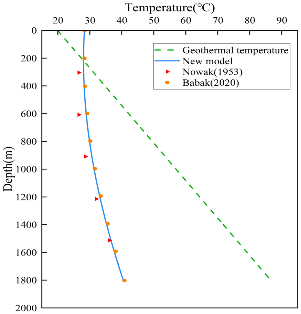
To address the above issues, this study first establishes a multilayer water absorption temperature profile prediction model that accounts for interlayer heterogeneity. The model couples multiple physical effects (including friction, Joule–Thomson, and thermal convection) as well as pipe flow and formation seepage. It overcomes the limitations of existing models that fail to couple the effects of reservoir multiphase flow and reservoir damage on the temperature profile. Then, the accuracy of the proposed model is verified by comparison with the Babak and Nowak models, and the influences of water injection rate, tubing inner diameter, permeability contrast, and skin factor on the temperature profile are analyzed. Finally, the model is applied to process distributed fiber optic temperature measurement data from Well A, achieving quantitative interpretation of water absorption in each sublayer. The research results provide a physically constrained quantitative analysis method for the application of distributed fiber optic temperature sensing monitoring technology in multilayer water injection well water absorption profile monitoring.

2. Construction and Solution of Temperature Profile Prediction Model for Water Injection Well

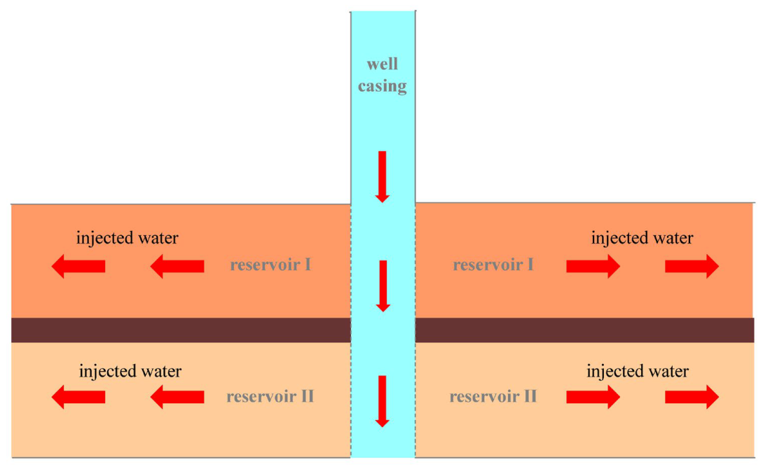
Based on the geological characteristics and physical parameters of the reservoir where the water injection well is located, and following the principles of mass and energy conservation, a prediction model for the temperature profile of multilayer water injection wells is established. This model comprehensively accounts for various factors, including frictional effects, the Joule–Thomson effect, thermal convection, and thermal expansion. During water injection, the injected fluid flows sequentially through two stages: the wellbore and the reservoir (Figure 1). In the wellbore, the flow is single-phase water, whereas in the reservoir, the presence of crude oil results in oil–water two-phase flow. Therefore, separate temperature field prediction models for the wellbore fluid and the reservoir fluid need to be developed, and an effective prediction of the wellbore temperature field is achieved through the coupled solution of these models.

In the process of water injection development in multilayered reservoirs, the physical properties of individual sublayers differ significantly due to sedimentation, diagenesis, and other factors. To establish a solvable mathematical model under reasonable simplifications while preserving the characteristics of interlayer heterogeneity, the following assumptions are proposed: (1) each sublayer is homogeneous with no interlayer cross-flow, and the fluid and rock are slightly compressible; (2) the oil–water two-phase flow is non-isothermal, with no physicochemical reaction between the phases; (3) the heat transfer medium is axisymmetrically distributed about the central axis of the tubing; (4) the pressure, temperature, and flow velocity are uniform across any given cross-section of the wellbore.

2.1. Fluid Temperature Prediction Model in Reservoir

When the injected water flows in the reservoir, considering the oil–water system in the formation, the flow equations of oil and water phases can be written as

$${\displaystyle \frac{1}{r}}{\displaystyle \frac{\partial }{\partial r}}\left[r\right({\displaystyle \frac{k{k}_{ro}}{{\mu }_o}}{\displaystyle \frac{\partial p_o}{\partial r}}\left){\rho }_o\right]+q_o={\displaystyle \frac{\partial }{\partial t}}\left(\varphi {\rho }_o{S}_o\right)]$$

(1)

$${\displaystyle \frac{1}{r}}{\displaystyle \frac{\partial }{\partial r}}\left[r\right({\displaystyle \frac{k{k}_{rw}}{{\mu }_w}}{\displaystyle \frac{\partial p_w}{\partial r}}\left){\rho }_w\right]+q_w={\displaystyle \frac{\partial }{\partial t}}\left(\varphi {\rho }_w{S}_w\right)]$$

(2)

where k is the formation permeability; k_ro and k_rw are the oil relative permeability and water relative permeability, respectively; μ_o and μ_w are the crude oil viscosity and formation water viscosity, respectively; ρ_o and ρ_w are the crude oil density and formation water density, respectively; S_o and S_w are the oil saturation and water saturation, respectively; p_o and p_w are the oil phase pressure and water phase pressure, respectively; q_o and q_w are the crude oil production rate and water injection rate, respectively; r is the radius; t is time; and φ is the porosity.

Due to the fact that the sum of oil and water saturation in the formation is 1, the equation can be written as

$$S_w+S_o=1$$

(3)

When the water injection is stable, the boundary conditions can be written as

$${\left(r{\displaystyle \frac{\partial p_w}{\partial r}}\right)}_{r=r_w}={\displaystyle \frac{q_w{\mu }_w{B}_w}{2k{k}_{rw}h}}+{\displaystyle \frac{q_w{\mu }_w{B}_w}{k{k}_{rw}h}}S$$

(4)

$$p{|}_{r=r_e}=p_i$$

(5)

where r_w is the wellbore radius; h is the formation thickness in meters; and S is the skin factor.

Since the reservoir is homogeneous within the sublayer and the pressure is equal everywhere in the formation, the initial condition can be

$$p(r,t){|}_{t=0}=p_i$$

(6)

When fluid flows through the reservoir, heat conduction also occurs. Based on the law of energy conservation and considering the effects of heat convection, heat dissipation, and heat conduction, if the heat transfer in the reservoir is steady-state, the energy conservation equation can be written as

$$-\left[\phi {\displaystyle \sum _i{\rho }_i{S}_i{C}_{pi}}+(1-\phi ){\rho }_m{C}_{pm}\right]{\displaystyle \frac{\partial T}{\partial t}}={\displaystyle \sum _i({\beta }_i{v}_i)T\frac{d{p}_i}{dr}}+{\displaystyle \sum _i{v}_i\frac{d{p}_i}{dr}+\lambda \frac{1}{r}(r\frac{dT}{dr})}$$

(7)

where C_p is the specific heat capacity of the fluid; C_pm is the specific heat capacity of the rock; ρ_m is the rock density; T is the temperature; β is the isobaric thermal expansion coefficient; v is the velocity; and λ is the thermal conductivity. The subscript i stands for oil or water.

2.2. Construction of Temperature Profile Prediction Model for Injection Well

In a water injection string, the flow is one-dimensional, and the forces acting on it can be classified into volumetric forces and surface forces. Volumetric forces act on all fluid particles and are proportional to the mass or volume of the fluid; they can act without direct contact. Examples include gravity, electromagnetic forces, and inertial forces. Surface forces act on the fluid surface and are proportional to the contact area, requiring direct contact for transmission. Examples include pressure, viscous forces, and surface tension. Under steady water flow conditions, the main forces are gravity, friction, and inertia, and the force balance can be expressed as follows:

$${\displaystyle \frac{dp}{dz}}={\rho }_{w}g\sin \theta -{\displaystyle \frac{f{\rho }_w{v}_w^2}{4r_t}}-{\rho }_w{v}_w{\displaystyle \frac{\partial v_w}{\partial z}}$$

(8)

where z is the axial coordinate; ρ_w is the water density; v_w is the water velocity; g is the gravitational acceleration; θ is the angle between the wellbore and the horizontal direction; f is the friction coefficient; and r_t is the radius of the water pipe.

Both the heat transfer inside the wellbore and that between the wellbore and the formation are considered transient processes; therefore, the same heat transfer equation cannot be used to describe the heat exchange between the wellbore medium and the formation. Instead, different heat transfer equations must be developed based on the distinct heat transfer modes of each medium within the wellbore. The temperature change in the injected water is influenced by factors such as friction, the Joule–Thomson effect, variations in physical properties, and pressure changes, whereas heat transfer in other media occurs primarily through thermal conduction and convective heat transfer. Taking the microelement of injected water in the wellbore as the analysis object, the main energy transfer modes include convective heat transfer, thermal conduction, work transfer, internal heat source transfer, and heat transfer through the tubing string. The corresponding expressions can be written as

$${\rho }_w{C}_{wp}{\displaystyle \frac{\partial T_w}{\partial t}}+{\rho }_w{C}_{wp}{v}_w{\displaystyle \frac{\partial T_w}{\partial z}}={\displaystyle \frac{\partial }{\partial z}}\left({\lambda }_w{\displaystyle \frac{\partial T_w}{\partial z}}\right)+{\displaystyle \frac{2h_1(T_t-T_w)}{r_t}}+{\displaystyle \frac{U_f}{{\pi r}_t^2}}+({\rho }_w{C}_{wp}{\alpha }_J+1){\displaystyle \frac{\partial p}{\partial t}}+({\rho }_w{C}_{wp}{\alpha }_J+1)v_w{\displaystyle \frac{\partial p}{\partial z}}$$

(9)

where λ_w is the thermal conductivity of the injected water; T₁ is the temperature of the fluid; T₂ is the temperature of the tubing column; α_J is the Joule–Thomson coefficient; and U_f is the heat generated by friction.

Frictional heat is absorbed by the fluid and the tubing string. The heat production formula is

$$U_f=qf{\displaystyle \frac{{\rho }_w{v}_w^2}{4r_t}}{\displaystyle \frac{b}{b+1}}$$

(10)

where q is the water flow rate; ρ_t is the density of the tubing string; and λ_t is the thermal conductivity of the pipe column. The expression for b can be written as

$$b=\sqrt{{\displaystyle \frac{{\lambda }_w{\rho }_w{c}_{wp}}{{\lambda }_t{\rho }_t{c}_{tp}}}}$$

(11)

The heat transfer modes of the pipe column mainly consist of convective heat transfer between the water and formation, axial heat conduction along the pipe column, and frictional heat generated between the water and the pipe wall. The heat transfer equation of the pipe column is as follows:

$${\rho }_t{c}_{tp}{\displaystyle \frac{\partial T_2}{\partial t}}={\displaystyle \frac{\partial }{\partial z}}({\lambda }_t{\displaystyle \frac{\partial T_2}{\partial z}})-{\displaystyle \frac{2r_1{h}_1(T_2-T_1)}{r_2^2-r_1^2}}+{\displaystyle \frac{2r_2{h}_2(T_3-T_2)}{r_2^2-r_1^2}}+{\displaystyle \frac{U_{f2}}{\pi (r_2^2-r_1^2)}}$$

(12)

where r₂ is the outer radius of the pipe column; h₂ is the natural convection heat transfer coefficient between the casing wall and the formation; T₃ is the base temperature; and U_f2 is the frictional heat absorbed by the oil tube.

During the water injection process, water flows from the wellhead to the formation, with substantial variations in temperature and pressure. Oil only flows within the formation, where the changes in temperature and pressure are relatively minor. To simplify the calculations, the model accounts for the effects of temperature and pressure on the density and viscosity of injected water. Considering the influence of temperature and pressure on water density, the density expression is given as follows [33]:

$$\begin{array}{l}{\rho }_w=1+1\times {10}^{-6}(-80T-3.3T^2+0.00175T^3+489P-2TP\\ \hspace{1em}\hspace{1em}+0.016T^{2}P-1.3\times {10}^{-5}{T}^{3}P-0.333P^2-0.002T{P}^2)\end{array}$$

(13)

The viscosity of water is calculated using the following formula [34]:

$${\mu }_w={\mu }_{w,i}\times \exp \left\{\left({\displaystyle \frac{0.068p}{100}}+0.0173\right){\left[\ln ({\displaystyle \frac{T}{125}})\right]}^2+\left(-{\displaystyle \frac{1.0531p}{100}}+0.0273\right)\left[\ln ({\displaystyle \frac{T}{125}})\right]\right\}$$

(14)

2.3. Coupled Solution of Temperature Distribution Model for Wellbore and Formation

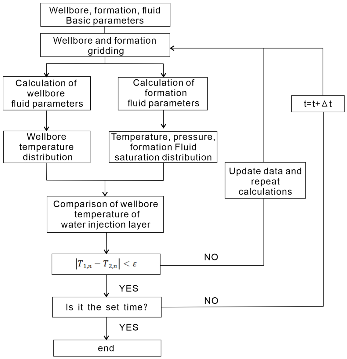
Based on the established reservoir fluid temperature prediction model, an exponential radial grid is adopted. Using the implicit pressure–explicit saturation method, the pressure field is first solved by simultaneously solving the oil–water equations, and then the saturation field is explicitly solved. Using the obtained saturation field and considering thermal convection and conduction, the temperature field is solved using the alternating direction implicit method, resulting in the discrete models for the reservoir fluid flow field and the reservoir fluid temperature field. For the wellbore temperature model, in the axial direction, the wellbore and formation are discretized with equally spaced grids, with nodes at the grid centers. In the radial direction, each of the three computational regions—the water column, the pipe string, and the borehole wall—contain one node, while nodes are radially equally spaced within the formation. Considering the different media and node spacings in the axial and radial directions of the wellbore, and to ensure equal heat flux across all control volume interfaces, the harmonic mean is used to handle the interface thermal conductivity and temperature gradient when solving, yielding discrete equations such as the wellbore temperature field discrete model. Based on the obtained discrete equations—namely the reservoir fluid flow field discrete model, the reservoir fluid temperature field discrete model, and the wellbore temperature field discrete model—Matlab 2020b programming is used to solve them. Given the formation conditions, the wellbore temperature distribution and the initial water injection rate for each sublayer are provided. The reservoir saturation field and temperature field distributions are then calculated. The temperature at the wellbore–formation boundary is compared, the initial water injection rate for each sublayer is updated, and the wellbore temperature field and reservoir temperature field are iteratively calculated until convergence. The specific calculation process is shown in Figure 2.

3. Model Validation

To validate the model’s accuracy, the developed water injection wellbore temperature model is compared with the computational results of the Babak model [35] and the Nowak model [36]. The calculations are performed under the following conditions: wellhead temperature of 28.33 °C, oil pipe diameter of 0.178 m, and injection rate of 155.52 m³/d. The results demonstrate that the model’s computational outcomes are largely consistent with those of the two other models and show particularly good agreement with the Babak model’s results (Figure 3). This comparative analysis thus confirms the accuracy of the wellbore temperature model.

4. Analysis of Influencing Factors on Wellbore Temperature Profile

Taking a multilayer water injection well as the research object, the temperature profile of the well is simulated and analyzed by the established prediction model. The influence of injection rate, parameters of tubing string, formation parameters and other factors on the temperature profile is evaluated. The basic parameters used in the simulation are shown in

Table 1. Reservoir parameters table.

Parameter	Value	Unit	Parameter	Value	Unit
reservoir depth	2000	m	formation pressure	20	MPa
porosity	15	%	rock density	2650	kg/m3
permeability	2	mD	rock heat capacity	850	J/(kg∙°C)
drainage radius	500	m	thermal conductivity	2.2	J/(m∙°C)
number of producing layers	3		geothermal gradient	0.03	°C/m

,

Table 2. Wellbore parameters table.

Parameter	Value	Unit	Parameter	Value	Unit
length	2000	m	wellbore diameter	0.25	m
tubing diameter	0.18	m	tubing inner diameter	0.16	m
wall roughness	0.00045	m	thermal conductivity	45	J/(m·°C)

and

Table 3. Formation parameters.

Layer	Top Depth /m	Bottom Depth/m	Thickness /m	Permeability /mD	Skin Factor
1	1650	1700	50	2	0
2	1800	1850	50	2	0
3	1950	2000	50	2	0

.

(1)

Effect of injection rate

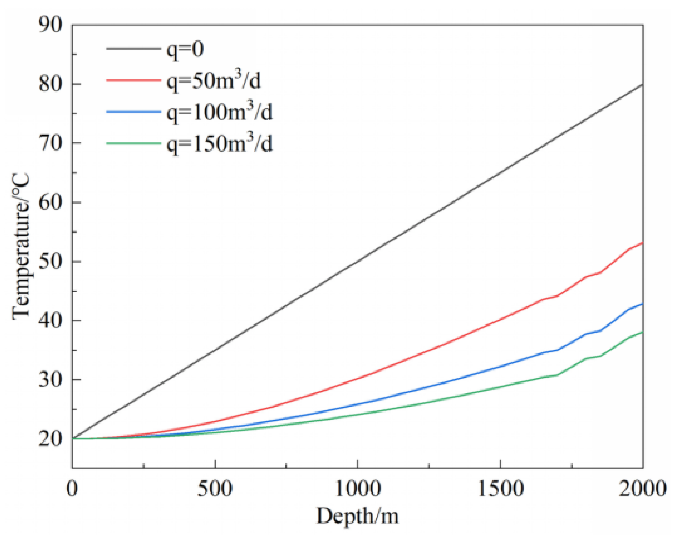
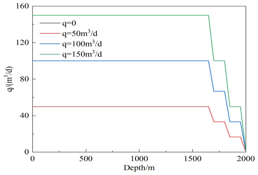
Since the temperature of the injected fluid is lower than the formation temperature, heat is transferred from the formation to the fluid. Figure 4 and Figure 5 show the temperature field distribution and flow field distribution in the wellbore, respectively. It can be observed that in non-water-absorbing layers, the higher the flow rate, the greater the deviation of the fluid temperature from the formation temperature. When the daily injection rate increases from 0 to 150 m³/d, the fluid temperature at a depth of 1600 m decreases from 65 °C to 28.75 °C. This occurs because heat transfer in non-water-absorbing layers is dominated by thermal conduction. With a higher flow rate, the fluid has a shorter contact time with the tubing wall, resulting in a smaller temperature rise. In water-absorbing layers, the temperature rise is significantly smaller than that in non-water-absorbing layers, and the greater the water intake, the smaller the temperature rise. As the daily injection rate increases from 50 to 150 m³/d, the temperature rise in the third sublayer decreases from 1.157 °C to 0.946 °C. This is mainly because heat transfer in water-absorbing layers occurs through both water convection and thermal conduction. The injection of low-temperature fluid into the formation reduces the formation temperature, thereby diminishing the heat transfer via both convection and conduction.

(2)

Influence of tubing diameter

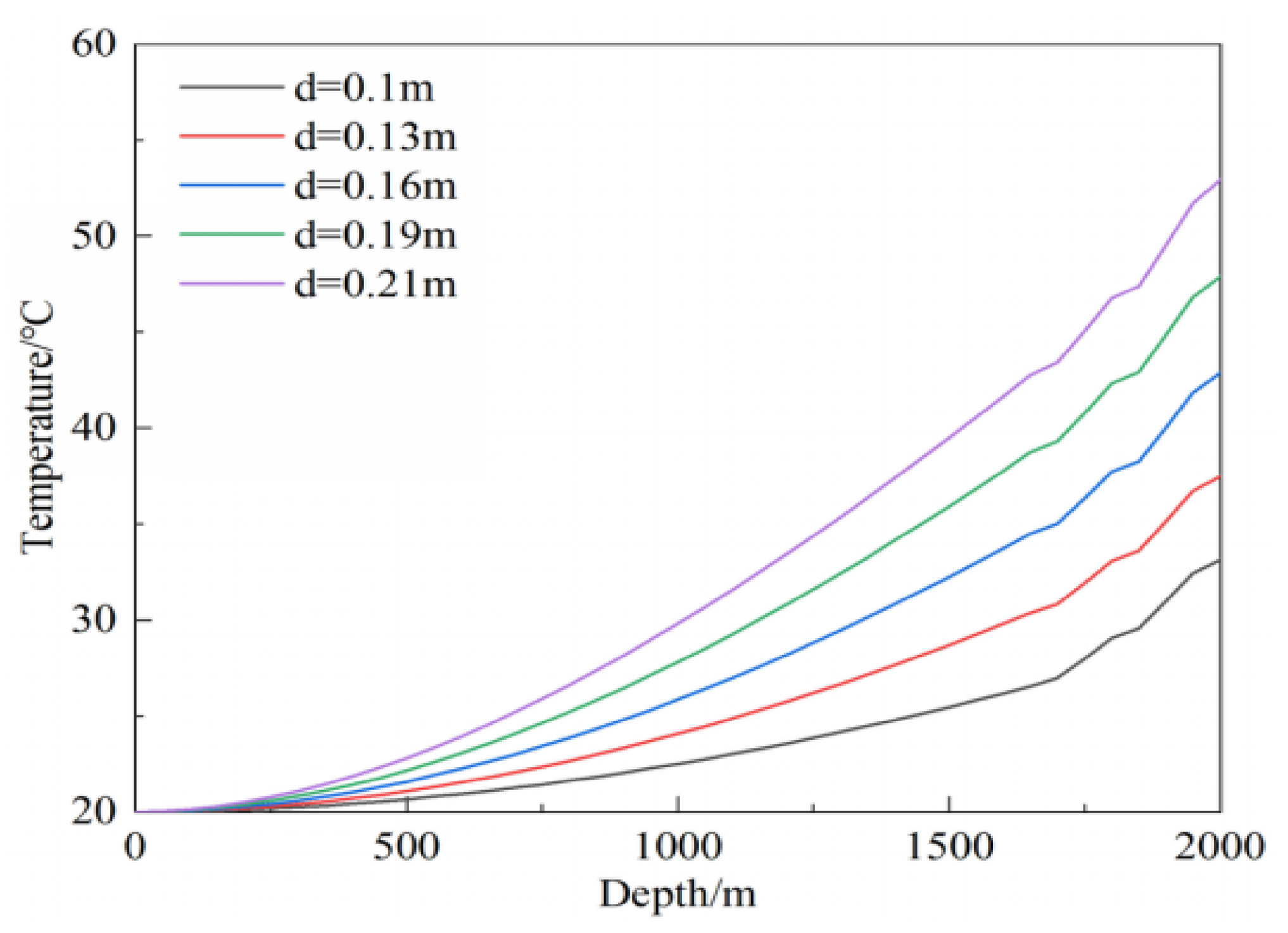
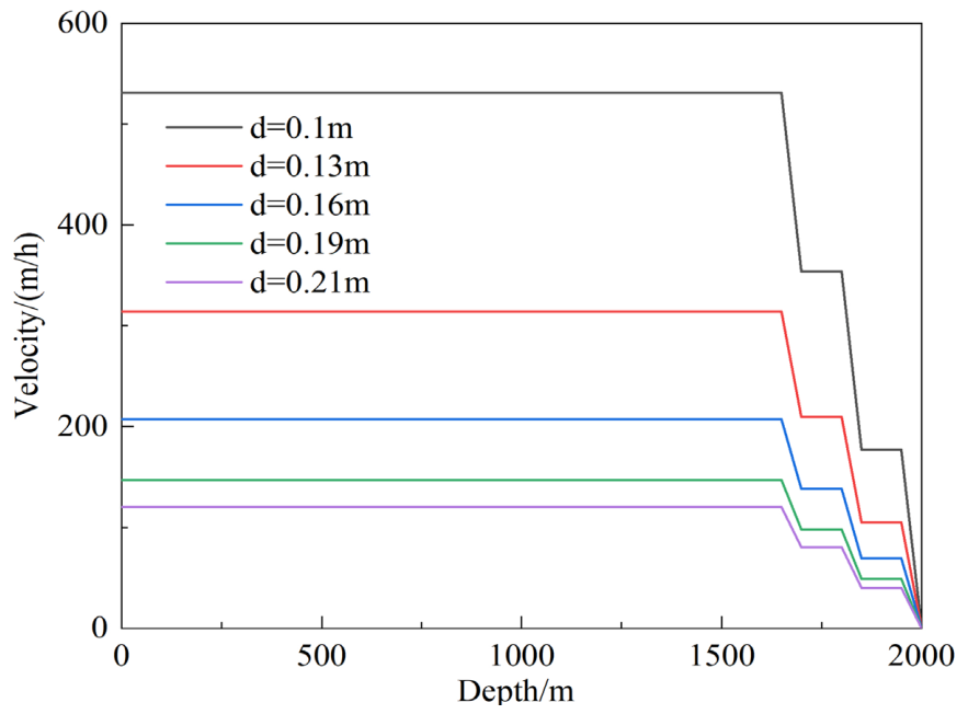
At a constant injection rate, the tubing inner diameter primarily affects the flow velocity of the injected water inside the tubing. Figure 6 and Figure 7 show, respectively, the temperature field distribution and fluid velocity field distribution of the wellbore at an injection flow rate of 100 m³/d. It can be observed from the figures that in the non-injection section, the change in fluid temperature is mainly caused by heat exchange between the fluid and the tubing and by frictional heating. The smaller the tubing diameter, the faster the fluid flows in the wellbore. When the tubing diameter increases from 0.1 m to 0.21 m, the flow velocity at a depth of 1600 m decreases by 76.2%. Although frictional heating increases, its overall contribution is relatively small, and the temperature rises from 26.169 °C to 41.651 °C. Therefore, the smaller the tubing diameter, the smaller the temperature rise. In the injection section, the temperature variation is smaller than that in the non-injection section, and the larger the injection rate, the smaller the temperature variation. This is mainly due to the fact that the injected fluid temperature is lower than the formation temperature.

(3)

Influence of formation coefficient

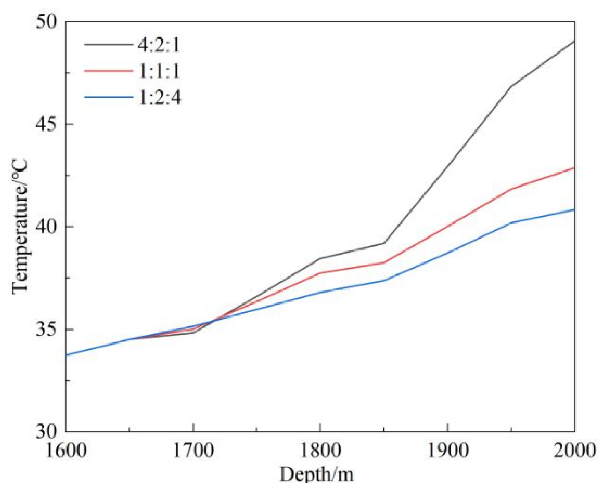
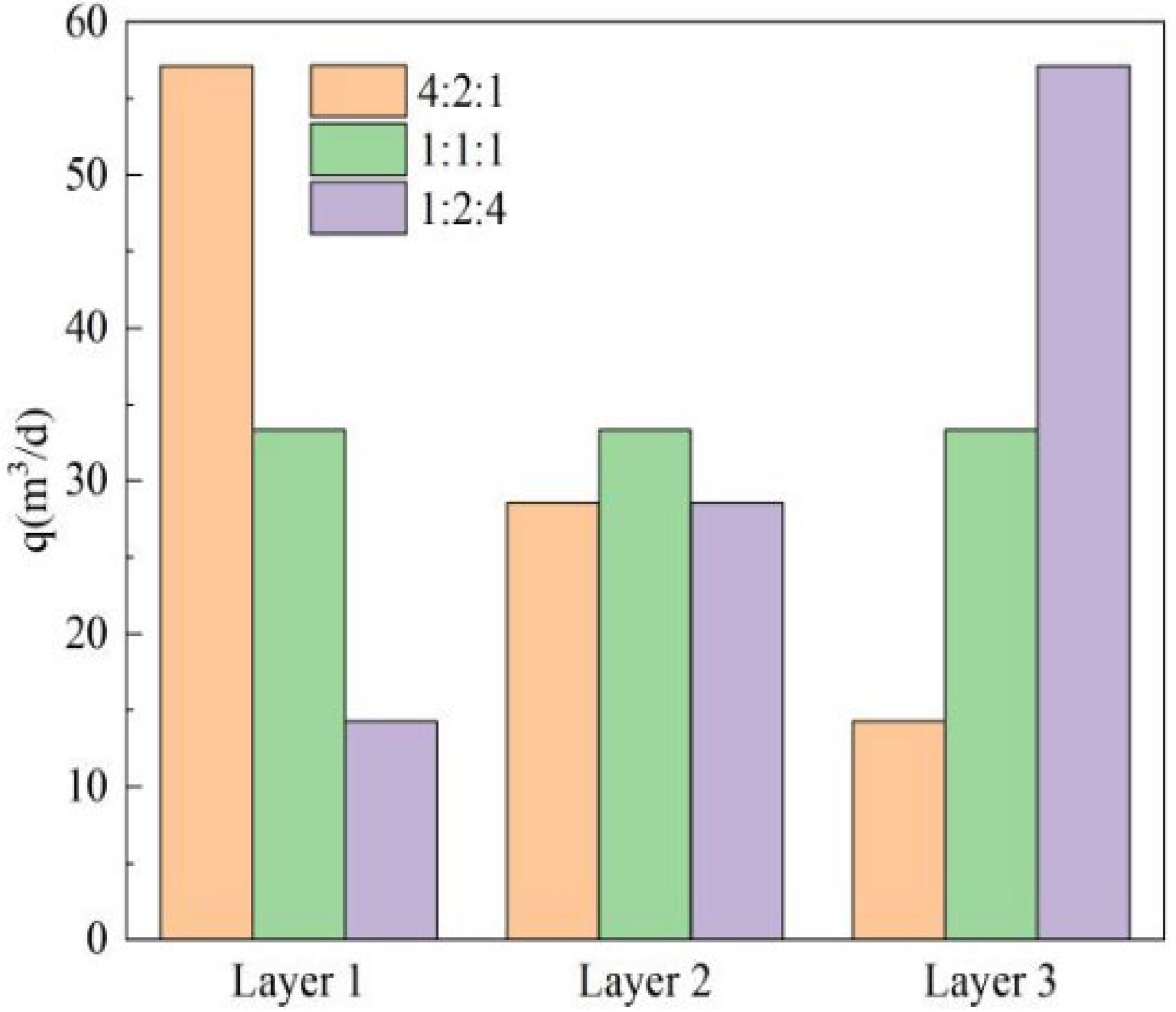
The formation coefficient is a key parameter for evaluating the fluid production capacity of a reservoir, defined as the product of the effective permeability and the effective thickness of the reservoir rock. During multilayer water injection, the formation coefficient mainly affects the water intake of each sublayer. To account for the influence of interlayer heterogeneity on the wellbore temperature field distribution, three representative formation coefficient ratios—4:2:1, 1:1:1, and 1:2:4—are selected. These represent, respectively, positive rhythm, uniform, and reverse rhythm variations in interlayer permeability. These three scenarios cover the possible trends in interlayer heterogeneity in actual reservoirs, thereby effectively revealing the influence of the formation factor distribution pattern on the temperature field. At an injection rate of 100 m³/d, the wellbore temperature field distributions for the three sublayers with formation factor ratios of 4:2:1, 1:1:1, and 1:2:4 are discussed separately. Figure 8 and Figure 9 show the wellbore temperature field distribution and the water intake histogram for each sublayer at an injection rate of 100 m³/d, respectively. When the formation factor ratio is 4:2:1, the water intake of the first sublayer is 57.14 m³/d, the second sublayer is 28.57 m³/d, and the third sublayer is 14.29 m³/d. Below a depth of 1700 m, the flow rate decreases, allowing for sufficient heat exchange between the fluid and the tubing. Consequently, the wellbore temperature rises significantly, increasing from 34.828 °C at 1700 m to 49.064 °C at 2000 m. When the formation factor ratio is 1:2:4, the water intake of the first sublayer is small, while that of the second and third sublayers is large. Below 1700 m, the flow rate remains high, resulting in a shorter heat exchange time between the fluid and the tubing. Therefore, the wellbore temperature rise is smaller, increasing only from 35.145 °C at 1700 m to 40.842 °C at 2000 m.

(4)

Influence of skin factor

The skin factor is a key indicator for evaluating reservoir damage, reflecting the additional pressure drop in a very thin annular region around the wellbore. It is equivalent to a coefficient derived by comparing the actual permeability of this region with the original formation permeability. During water injection, reservoir damage often occurs due to factors such as injection water quality and reservoir sensitivity, which increase the flow resistance for fluid entering the formation. 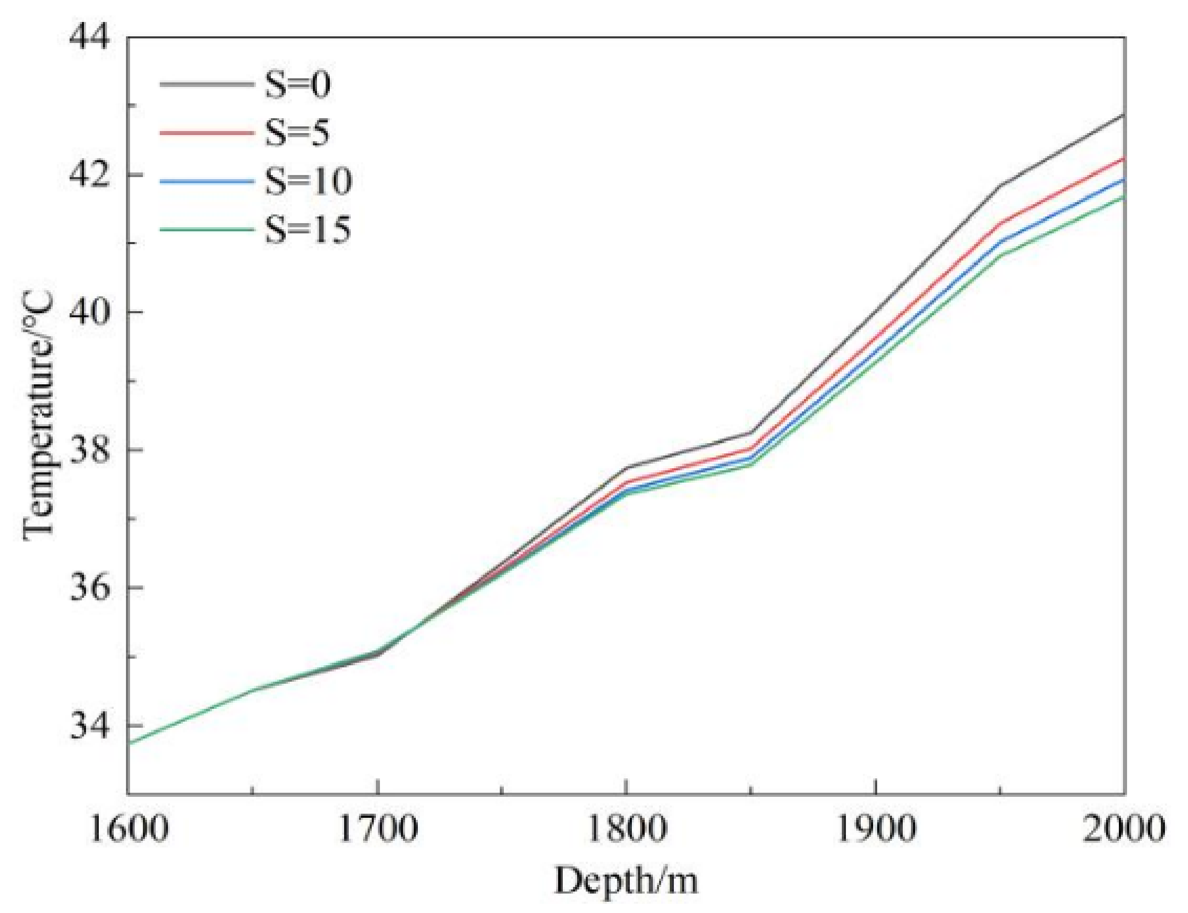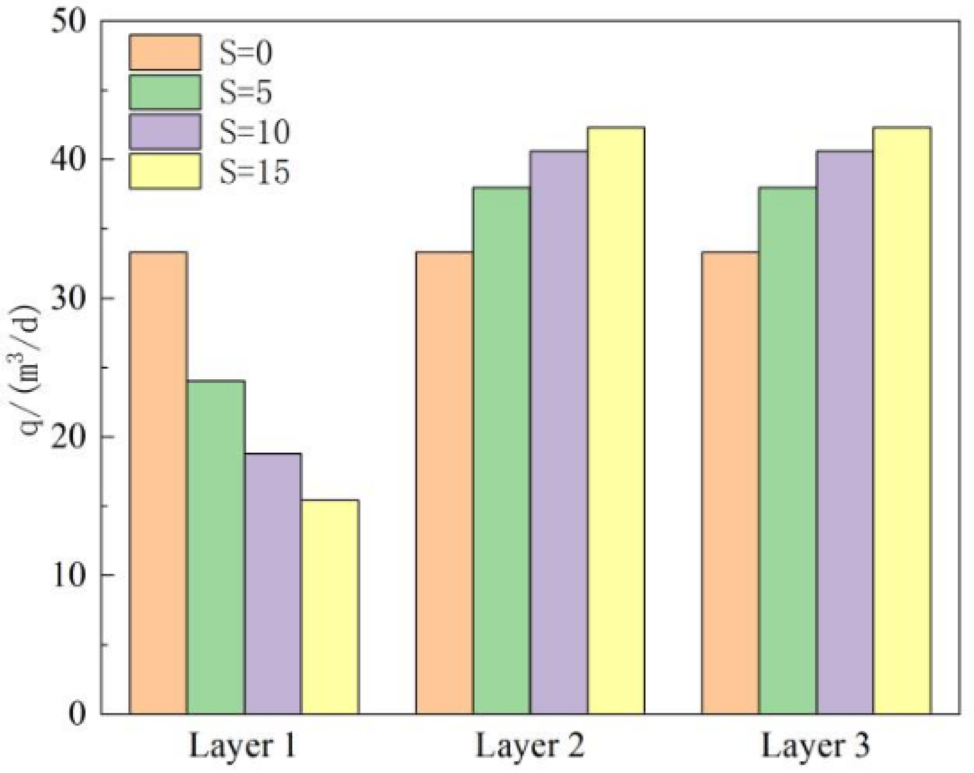Figure 10 and Figure 11 show, respectively, the wellbore temperature field distribution and the water intake histogram for each sublayer in a multilayer injection well with the same formation factor, at an injection rate of 100 m³/d, under different skin factors in the first sublayer. When the skin factor of the first layer increases, the flow resistance in that layer increases, and the injection rate decreases. As the skin factor increases from 0 to 15, the water intake of the first sublayer decreases from 33.33 m³/d to 15.43 m³/d, and the temperature at 1800 m drops from 37.73 °C to 37.35 °C. Under the tested conditions, the overall temperature pattern change is smaller than the changes caused by flow rate or tubing diameter, but the skin factor still affects local flow and temperature behavior.

5. Example Application

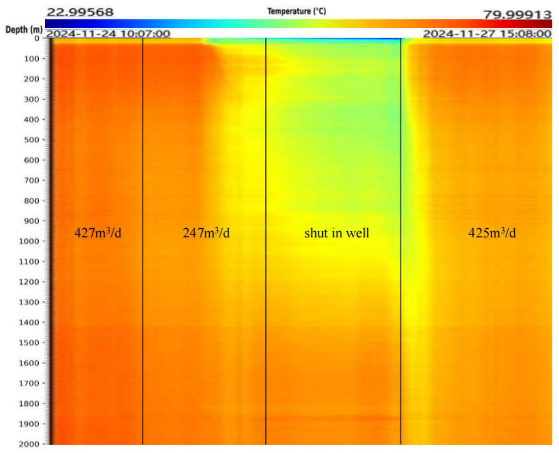
Well A is a water injection well in the Bohai Oilfield, with a total water absorption layer length of 224 m. Between March 21 and 31, 2024, the well underwent tubing string replacement, with balanced water injection and fiber optic tubing installed. From 24 to 27 November 2024, distributed fiber optic temperature measurements were conducted. During the tests, continuous temperature response data was collected across the entire wellbore under various production regimes, with corresponding data obtained for both shut-in conditions and rates of 240 m³/d and 430 m³/d. The monitoring process, which involved three systems, lasted approximately 76 h. The temperature acquisition waterfall diagram is shown in Figure 12.

After completion of the operations, DTS test data interpretation was carried out based on the temperature response data acquired under the conditions prior to shut-in temperature recovery. Using the established temperature profile prediction model for water injection wells, it can be observed that due to the temperature difference between the injected water and the formation, the wellbore temperature gradient in the injection well deviates from the geothermal gradient. Under different tubing configurations, the temperature profile within the injection well exhibits different patterns. By analyzing the changes in flowing fluid temperature across different reservoir intervals, the water absorption capacity of each interval is determined. Based on the multilayer water absorption temperature profile calculation model for water injection wells constructed in this paper, the wellbore and formation are discretized into a grid: the wellbore grid step size is 1 m, and the formation is divided into 20 radially exponential grid nodes. Combining regional wellbore, formation, and fluid parameters, the wellbore model and the formation model are coupled to solve the forward fitting of the water absorption profile, thereby obtaining the water injection rate for each injection interval. Since identifying the interface between water-absorbing and non-water-absorbing layers from the temperature curve is challenging, the water absorption intervals are corrected using logging interpretation results, as presented in

Table 4. Interpretation results of distributed fiber optic temperature sensing logging in Well A.

Sandstone Depth (m)	Sandstone Bottom Depth (m)	Thickness (m)	Absolute Injection Volume (m3)	Relative Injection Amount (%)
1840.7	1853.2	12.5	13.30	3.13
1878.7	1897.5	18.8	129.70	30.57
1910.2	1914.1	3.9	15.60	3.68
1929.5	1950.6	21.1	103.00	24.28
1963.3	1965.4	2.1	12.80	3.02
1975.8	1984.2	8.4	25.40	5.99
1994.2	2001.5	7.3	48.90	11.52
2013.6	2018.5	4.9	15.60	3.68
2025.6	2029.8	4.2	46.50	10.96
2035.2	2038.6	3.2	13.50	3.18
amount to			424.3	100

. The test results show that the main water-absorbing intervals of the well are 1878.7–1897.5 m and 1919.5–1950.6 m, with water absorption accounting for 30.57% and 24.28% of the total injection rate, respectively, while the remaining measured depth intervals exhibit secondary water absorption. Oxygen activation logging was performed on the tested intervals six months ago. At an injection rate of 350 m³/d, the relative water intake for the main intervals (1878.7–1897.5 m, 1919.5–1950.6 m, 1994.2–2001.5 m, and 2025.6–2029.8 m) was 34.32%, 28.45%, 10.37%, and 7.32%, respectively. The main interval interpretation results from DTS testing are generally consistent with those from oxygen activation logging, confirming the reliability of the DTS-based interpretation.

6. Conclusions

(1) Considering interlayer heterogeneity and reservoir damage, this paper constructs a temperature profile prediction model for water injection wells based on the laws of conservation of mass and energy. The model comprehensively accounts for the effects of friction, the Joule–Thomson effect, thermal convection, and thermal expansion and couples wellbore pipe flow with formation seepage. This model enables accurate prediction of the steady-state wellbore temperature profile under water injection conditions, laying a theoretical foundation for inverting the water injection profile using temperature profile monitoring data.

(2) Water injection rate and tubing diameter are the main factors controlling the water flow velocity in the casing, thereby influencing the temperature field distribution in the wellbore. A higher injection rate results in a shorter contact time between the fluid and the tubing wall, leading to a smaller temperature rise in the injected water. Conversely, a larger tubing diameter slows down the water flow velocity within the tubing string, causing a greater temperature rise in the injected water. The formation coefficient determines the distribution of water absorption among individual sublayers, while the skin factor primarily affects the allocation of injection rate across these sublayers.

(3) For Well A, the main water-absorbing intervals are 1878.7–1897.5 m and 1919.5–1950.6 m, with water absorption accounting for 30.57% and 24.28% of the total injection rate, respectively. The remaining measured depth intervals exhibit secondary water absorption. These interpretation results are in good agreement with earlier oxygen activation tests, verifying the reliability of the proposed model and interpretation method.

(4) The model presented in this paper is primarily developed for steady-state water injection conditions and does not consider the dynamic evolution of temperature responses during transient processes such as shut-in or start-up. Furthermore, the current work is only applicable to Newtonian fluids such as brine and has not yet addressed the complex thermal–hydraulic–chemical coupling behaviors associated with the injection of non-Newtonian fluids (e.g., polymer solutions and surfactants). These aspects require further improvement in future research.