Synthesis of Decision Logic for Predictive Maintenance of a Marine Diesel Engine Based on Unconditional Control-Reliability Indicators

Abstract

This paper proposes a formal framework for synthesizing multi-stage condition-based maintenance (CBM) decision logic for marine diesel monitoring systems. The design object is treated not as a single threshold or classifier output, but as an implementable decision logic with explicit stages of data-quality gating, thresholding, confirmation, fusion, and temporal filtering. Decision quality is evaluated using unconditional control-reliability indicators (CRIs) under a prescribed prior probability of rare abnormal events within a unified Monte Carlo verification protocol. Within a simplified Gaussian surrogate model, we compare baseline thresholding, repeated-measurement averaging, within-path confirmation, and measurement-level fusion. For the reported reference configuration, averaging five repeated measurements yields the largest reduction in the raw error criterion, “2 out of 3” confirmation provides a smaller but consistent improvement, and two-path multi-fidelity fusion is beneficial only after calibration toward the more informative path. The results show that, under rare abnormal events and limited measurement accuracy, decision quality is determined primarily by calibration of the multi-stage channel-level logic rather than by thresholding alone.

1. Introduction

Marine diesel engines and their air-handling systems operate over long voyages under variable operating conditions and strict, safety-driven constraints on intervention [1,2,3]. In this setting, degradation and incipient faults often develop amid normal parameter fluctuations, while failure events and labeled fault cases are rare and thus underrepresented in operational datasets [4,5,6]. Therefore, the practical task of early abnormality detection (anomaly detection, AD) and subsequent fault diagnosis (FD) is addressed within a condition-based maintenance (CBM) framework (often referred to in industry as predictive maintenance, PdM), where transparent and reproducible decision logic is as important as model accuracy [7,8,9].

In contemporary PdM practice, the observable quantity that triggers decisions is frequently not a raw measurement but a diagnostic statistic computed by a normal-behaviour or state-estimation AI/ML (artificial intelligence and machine learning) model (e.g., a residual, an autoencoder reconstruction error, or an anomaly score) [10,11]. Such model-derived statistics are attractive under limited instrumentation, yet their outputs are uncertain, operating-condition dependent, and prone to spurious excursions; therefore, they require explicitly specified thresholding, confirmation, and fusion rules with controlled error risks. This paper addresses the engineering interface between AI/ML-based AD/FD modules and the shipboard cyber–physical monitoring loop by synthesising decision logic that converts model outputs into reproducible maintenance triggers.

A practical feature of shipboard CBM is limited data quality and availability. Using operational data from an in-service vessel, Upadrashta and Wijaya showed that datasets can be sparse, noisy, and incomplete [10]. They also presented an end-to-end CBM architecture spanning sensors, onboard edge computing, cloud services, and a monitoring dashboard, including a pragmatic workaround for limited parameter access via image-based acquisition from display screens when direct interfaces are unavailable [10]. The set of feasible monitoring signals is therefore often constrained by what can be accessed onboard (see

Table 1. List of available monitoring parameters [10].

Engine Parameters	Turbocharger Parameters
Engine generator status	Turbine inlet gas temperature
Engine RPM	Turbine outlet gas temperature
Engine load	Turbocharger speed
Voltage and Amperage	Bearing and lubrication system parameters
Charged air pressure	Lubrication oil pressure
Charged air temperature	Lubrication oil inlet temperature
Engine start pressure	Bearing temperature
Engine cylinder (1–6) temperatures	Cooling system parameters
Fuel injection system parameters	Cooling water pressure
Fuel oil pressure	Cooling water temperature (inlet and outlet)
Fuel oil temperature	Vibration
Fuel oil mass flow rate	Time series and frequency domain features

for an example). Related CBM architectures are described in [12,13].

A second persistent source of uncertainty is the rarity of failure cases and the resulting class imbalance [14,15,16]: normal observations far exceed failure-related observations, so conventional accuracy metrics can overestimate performance and understate operational risk [17]. For marine main-engine diagnostics based on operational data, the shortage of failure examples and the need to account for it during model development and validation are emphasized in [11]. Studies focused on adapting to imbalanced datasets and updating models during operation show that imbalance can be mitigated algorithmically (e.g., via synthetic data augmentation and feature dimensionality reduction), yet this alone does not guarantee controlled risks of false alarms and missed detections in service [18].

Marine diagnostics is almost always multichannel and multi-fidelity [19,20,21]. Some parameters are measured directly, whereas others are available only through proxy indicators or with limited accuracy; therefore, the set of monitoring channels is largely determined by engineering feasibility and measurement cost [22]. Applied studies emphasize that simple, operationally feasible proxy indicators (e.g., combustion-process and fuel-consumption parameters) can support condition monitoring without invasive measurements [23,24,25]. In parallel, non-traditional sources (e.g., generator electrical signals and their spectral descriptors) have been shown to improve observability without increasing physical access requirements to engine components [26,27,28]. Given this diversity of measurement paths, a central question is how to fuse heterogeneous evidence and make reliable decisions under conflicting, incomplete, or noisy observations [29,30,31].

Related work also considers formalised decision making under deployment constraints, data uncertainty, and asymmetric error costs. In marine applications, optimisation models and simulation-based analyses have been used to select decisions under time, cost, and technical constraints [32,33,34,35,36]. Decision criteria under uncertainty are supported by scenario analysis and economic performance indicators [37,38], while the interpretation of losses and managerial consequences is developed in methods for economic assessment of resource losses [39]. From a safety perspective, multi-stage strategies are used when adverse outcomes are costly, which is methodologically consistent with confirmation and escalation in CBM decision logic [40]. Related work on proxy modelling and computationally efficient models further supports treating diagnostic quantities as computed indicators that must be embedded into a multi-stage decision logic [25,41,42]. Practical deployability is illustrated by implemented monitoring systems [43,44] and by engineering solutions aimed at reducing intervention frequency and improving process efficiency [45,46,47]. Finally, the need for reproducible tuning is reinforced by changes in operating profiles caused by alternative diesel-fuel components (biodiesel/green diesel) [48,49] and the associated shifts in diagnostic-indicator statistics [50,51,52].

CBM decision making for a marine power plant is considered here under three practical constraints: limited deployability and data accessibility onboard, severe class imbalance due to failure rarity, and heterogeneous (multi-fidelity) measurement quality. The task is to define a channel-level logic that maps the observed statistic Z to an alarm/no-alarm decision and to compare how thresholding, averaging, confirmation, and fusion change $\alpha$, $\beta$, and $J_{\mathrm{err},\mathrm{raw}}$ under the same uncertainty model.

As a reference context, we use the practical two-stage “AD–FD” setup and the end-to-end (E2E) CBM architecture demonstrated on an in-service vessel in [10]. Within this context, Section 3 formulates the proposed decision logic and evaluates selected mechanisms through unconditional control-reliability indicators (CRIs) in a Monte Carlo setting.

The goal of this paper is to synthesise a CRI-based CBM decision-logic framework for marine diesel engines and to verify selected logic components via Monte Carlo simulation on a simplified Gaussian surrogate model. The main contributions are as follows:

• A formal design framework is proposed in which the object of synthesis is an implementable multi-stage CBM decision logic rather than a single threshold or classifier output;
• Decision quality is quantified by unconditional control-reliability indicators (CRIs), allowing channel-level logic variants to be compared under an explicit rare-event prior and controlled operating uncertainty;
• A structured channel description is introduced that makes the logic parameters explicit, including repeated measurements, within-path confirmation, multi-fidelity aggregation, and temporal filtering;
• Selected logic elements are compared within a unified Monte Carlo verification protocol, which enables direct assessment of how pre-binarisation and post-binarisation mechanisms change false-alarm and missed-detection risks;
• The framework is positioned as a downstream layer between AI/ML-based AD/FD modules and maintenance action, providing a basis for later validation on operational marine data.

2. Related Work

Studies on condition-based maintenance (CBM) for marine diesel engines and their subsystems, often discussed in practice under the broader label of predictive maintenance (PdM), develop along several applied lines. These include shipboard deployment under limited data accessibility, two-stage “anomaly detection–fault diagnosis” workflows under failure rarity, rule- and threshold-based maintenance decisions, and model-centric diagnostic systems that report strong classification metrics but leave the operational decision layer only partly specified.

Because the present paper focuses on decision logic evaluated through unconditional control-reliability indicators (CRIs), the review below concentrates on the parts of prior work that are methodologically most relevant for this task: practical deployment constraints, threshold-based triggering, confirmation procedures, state zoning, uncertainty of measurements and proxy indicators, and the possibility of combining channels with unequal fidelity within an implementable maintenance-triggering logic.

2.1. Deployment Constraints and Data Availability in Shipboard CBM/PdM

One of the most practice-oriented end-to-end CBM/PdM pipelines based on operational data is presented by Upadrashta and Wijaya [10], who study an in-service marine diesel engine under explicitly stated limitations in data quality and completeness. The importance of this work lies not only in the use of anomaly-detection and classification models as such, but also in the direct demonstration of actual shipboard constraints: parameter acquisition, local processing, data transmission, diagnostic interpretation, and the construction of labelled fault scenarios with severity grading. In methodological terms, this is important because it places classification and maintenance decisions inside a real monitoring chain affected by incomplete observations, heterogeneous signals, and class imbalance.

The set of monitored engine and turbocharger parameters reported in [10] is summarised in Table 1. This list is useful not as a descriptive inventory alone, but as an illustration of the practical channel set available in shipboard monitoring: a mixture of directly measured variables and proxy indicators with different noise levels, sampling properties, and diagnostic informativeness. Such heterogeneity motivates treating marine monitoring as a multi-channel and, in a broader sense, multi-fidelity decision problem rather than as a single-signal thresholding task.

From the viewpoint of the present study, this type of deployment context is fundamental because it shows that the decision problem in marine CBM/PdM is not limited to selecting a classifier. It also requires an explicit logic for handling channel heterogeneity, imperfect measurements, and operational triggering under rare adverse conditions.

2.2. From Anomaly Scores to Maintenance Decisions: Thresholds, Confirmation, Zones, and Fusion

A central methodological line directly related to decision-logic synthesis is the two-stage workflow in which anomaly detection is trained on data representing healthy operation, while fault diagnosis is performed only after failure data become available or are progressively accumulated [53,54,55]. In [10], this idea is implemented explicitly: abnormality detection is based on the reconstruction error of an autoencoder with a threshold of the form $T={\mu }_E+k{\sigma }_E$, after which supervised diagnosis is performed across fault classes and severity levels. Even in this relatively standard form, thresholding already acts as a first-level decision rule and therefore directly influences false-alarm and missed-detection behaviour near the boundary of normal fluctuations, especially under early-stage degradation and severe class imbalance.

A related line is represented by model-centric diagnostics that operate with a limited set of informative signals and achieve high test-set performance but leave the downstream decision structure comparatively implicit. Kim et al. [11], for example, diagnose a low-speed marine main engine from exhaust-gas temperature using a hybrid deep-learning model. Two aspects are especially relevant here. First, the authors explicitly consider controlled overlap between classes, which is consistent with increasing decision uncertainty under degradation, noise, and blurred state boundaries. Second, despite the claimed real-time applicability, the final output remains essentially a model-level class label rather than a maintenance-triggering logic with explicit re-check, confirmation, escalation, or persistence rules.

Another important line is formed by rule-based and zone-based approaches, in which the maintenance decision is represented not only through a score or class label but through interpretable operating regions associated with actions. In [56], Karatug et al. propose a hybrid strategy combining condition-based maintenance with reliability-centred maintenance by partitioning the time to functional failure into zones such as ideal state, warning, pre-failure, and failure. The importance of this approach for the present paper lies in the structure of the decision itself: each zone corresponds to an action class, which makes the logic operationally meaningful even when the boundaries between zones are not explicitly calibrated through probabilities of false alarms and missed detections.

Under scarce failure data, a closely related strategy is residual-based monitoring, where a model of normal behaviour is first constructed and alarms are then generated from deviations relative to thresholds or fault boundaries. This line is illustrated by Ceglie et al. [57], where an artificial neural network is trained on normal data and fault boundaries are formed from simulation results; an alarm is issued when several residuals jointly enter a region interpreted as fault-related. Methodologically, such formulations are important because they naturally motivate confirmation over observation sequences and the explicit use of alarm history when noise, transients, or operating-condition variability can produce spurious single-point decisions.

Additional motivation for an explicit multi-fidelity decision layer comes from studies based on proxy indicators and indirect measurements, which recognise that ideal diagnostic channels are often unavailable in practice. Duc Nghia et al. [58] relate fuel-injection parameters to smoke and soot as practical diagnostic indicators, while Markelova and Ivanovskaya [23] discuss diagnostics based on indirect indicators with explicit threshold rules under shipboard measurement constraints. From another perspective, Gasparjans et al. [26] use generator electrical quantities and spectral descriptors as an alternative diagnostic path. By contrast, works primarily focused on class imbalance and model adaptation address algorithmic robustness, for example through deep Q-network (DQN)-based diagnosis on simulated data [59] or through schemes based on the Borderline Synthetic Minority Over-sampling Technique (BorderlineSMOTE), kernel principal component analysis (KPCA), and online sequential extreme learning machine (OSELM) with online updating [18], but usually leave heterogeneous channel trust, confirmation, and action logic only implicit. Taken together, these studies support the need for a separate decision-logic layer capable of comparing, calibrating, and combining channels of unequal fidelity under incomplete and noisy observations.

2.3. Methodological Gap and Positioning of This Paper

The reviewed literature indicates a recurring gap between model-centric diagnostics and operational maintenance decision making. In many studies, the effective decision layer is reduced to a single threshold on an anomaly score, residual, or classifier output, whereas confirmation, escalation, temporal persistence, and multi-channel fusion remain only partly specified or are absorbed implicitly into the model architecture.

In the present paper, we therefore treat the decision logic itself, together with its structure and parameters ${\theta }_i$, as the design object. The proposed formulation is methodologically close to classical tools such as Type I/Type II error analysis and ROC-style reasoning, but it differs in one essential respect: for shipboard application, the object to be calibrated and compared is not a single threshold or classifier score but an implementable decision logic composed of channel-level operations.

More specifically, the contribution is formulated as a decision-layer synthesis framework in which thresholding, repeated-measurement averaging, within-path confirmation, measurement-level fusion, and temporal filtering can be structured, tuned, and compared under a common probabilistic verification protocol using unconditional CRIs. In this sense, the paper is positioned not as another classifier-evaluation study, but as a formal and reproducible scheme for maintenance-trigger design under rare abnormal events, limited measurement quality, and heterogeneous diagnostic channels.

3. Materials and Methods

3.1. Formalising CBM as a Condition Monitoring and Decision-Making Problem in a Multichannel Multi-Fidelity System

CBM for a marine diesel engine is formulated as a condition monitoring and decision-making problem under (i) failure rarity, (ii) operating-condition variability, and (iii) heterogeneous measurement quality. CBM is treated not as “a single classifier model”, but as a reproducible decision logic that, based on available observations, produces a binary decision—no alarm ($\overline{A}$) or alarm (A)—and, when required, triggers subsequent fault diagnosis (FD) to identify the likely cause. In the present paper, this logic is treated as a formal design language for maintenance triggering, in which the structure of decision stages and the associated parameters are explicit design variables subject to verification through CRIs.

Terminology and scope. Unless stated otherwise, terminology follows ISO 13372 and ISO 2041, while the general CM/diagnostics workflow is interpreted in line with ISO 17359 [60,61,62]. In ISO 13372, predictive maintenance is deprecated in favour of condition-based maintenance; throughout the paper, “PdM” is used only as an industry synonym. We use fault for a state and failure for an event (loss of function), consistent with ISO usage. Finally, the proposed control-reliability indicators quantify correctness of monitoring decisions (TN/TP/FA/MD) and should not be confused with equipment reliability in the ISO sense.

The following definitions and notations are used.

Diagnostic variable $X_i$. The diagnostic variable $X_i$ is the quantity used to infer the state of a component or subsystem and detect abnormalities. The variable $X_i$ can be (i) a physical parameter (e.g., charged-air pressure, exhaust gas temperature (EGT), turbocharger speed) or (ii) a computed diagnostic indicator (descriptor), such as a residual, reconstruction error, or anomaly score, obtained from measurement data and a model. In ML-enabled CBM/PdM, such computed indicators are typically the direct outputs of AI/ML models trained to represent normal behaviour or to estimate state from limited signals; in this case, the monitoring channel operates on a model-derived statistic rather than on a single physical measurement.

Measurement path j. A measurement path j is a specific route by which an estimate of $X_i$ is obtained, including the sensor, signal conversion, transmission, computation, and preprocessing. The path is characterized by the resulting error $Y_{ij}$ and, in the general case, by delays, missing data, and noise. The measurement outcome in path j is described by the model:

$$Z_{ij}=X_i+Y_{ij},$$

(1)

For computed diagnostic statistics, Equation (1) is treated as an estimation-error model: $X_i$ denotes the latent (true) value of the diagnostic indicator, whereas $Y_{ij}$ is an aggregate random term that represents the combined uncertainty introduced along measurement path j. This term subsumes instrumentation and acquisition effects (measurement noise, calibration changes, time misalignment, missing-data handling) as well as processing and modelling effects (preprocessing, feature extraction, operating-condition normalisation, and model mismatch).

Accordingly, when $X_i$ is a directly measured physical parameter, $Y_{ij}$ is dominated by instrumentation and acquisition uncertainty; when $X_i$ is a computed diagnostic statistic (e.g., a residual of a normal-behaviour model, an autoencoder reconstruction error, or an anomaly score), $Y_{ij}$ also includes the approximation error of the underlying model and the variability introduced by preprocessing. In all cases, $Z_{ij}$ is the observable diagnostic quantity used for decision making in a monitoring channel, and a decision region $\omega$ is defined in the space of $Z_{ij}$.

Regardless of whether $Z_{ij}$ is a physical measurement or an AI/ML-derived diagnostic statistic, the operational task is to map $Z_{ij}$ to a reproducible alarm/no-alarm decision with controlled risks. In this formulation, the CRI-based layer is placed downstream of the AI/ML module and upstream of maintenance actions, which is typical of cyber–physical PdM systems.

Monitoring channel i. A monitoring channel i aggregates one or more measurement paths j used to monitor a single diagnostic variable $X_i$. A channel may include multi-fidelity measurement paths, for example, a “high-accuracy” sensor and a “coarse” or indirect source, different sensor types, or a combination of a measurement and a model-based estimator.

Proxy indicator. A proxy indicator is a quantity that does not coincide directly with $X_i$ but is informative about the system state. Proxies may be direct measurements (e.g., generator electrical quantities) or derived descriptors (e.g., RMS, kurtosis, spectral peaks of a vibration signal, or time-series statistics). Proxies are introduced either as separate diagnostic variables $X_i$ or as an additional measurement path within a channel when the proxy is used for confirmation or refinement.

Fusion. Fusion denotes a rule for combining evidence across measurement paths within a channel and/or across channels of the overall system. Fusion is used broadly, ranging from simple logical combination (e.g., “a out of m”, majority voting, averaging, or weighted fusion) to multi-level aggregation of decisions (e.g., confirmation over observation sequences, alarm escalation, and consistency checks between independent channels).

The complete list of symbols and notation is summarized in Appendix A.

From a decision-making perspective, each monitoring channel produces a binary decision based on the observation(s) $Z_{ij}$:

• $\overline{A}$: no alarm;
• A: alarm.

At the CBM level, the decision is constructed in a multi-stage manner. First, a data quality gate is applied. Next, threshold checks are performed at the measurement-path level. This is followed by confirmation using repeated measurements, repeated decision cycles, or an alternative measurement path. The workflow may then proceed to the two-stage “AD–FD” separation (abnormality detection followed by fault diagnosis). Finally, the logic aggregates evidence across channels via fusion and issues an action (observe/alert/intervene).

In the subsequent methodology, solution quality is not defined solely through model metrics; it is quantified using probabilistic indicators of decision correctness—the risks of false alarms and missed detections—in an unconditional setting, i.e., accounting for typical operating conditions and failure rarity. This provides a direct link between decision-logic design and verifiable operational requirements.

3.2. Object and Data/Signal Loop

The application context of this study is a marine diesel engine and its air-handling system, including subsystems that affect cylinder charging, thermal conditions, and turbocharging operation. The data loop comprises measurements available from the ship’s standard automation system and/or additional monitoring devices; the available channels, sampling rates, and data completeness depend on the specific vessel and interface implementation.

To ensure comparability under variable operating conditions, the diagnostic variables $X_i$ are interpreted in the context of operating conditions (load, speed, and thermal conditions). Consequently, within the CBM logic, some thresholds and confirmation criteria are defined not in absolute terms, but as functions of operating conditions or as deviations from expected normal behaviour at a given operating condition (e.g., via residuals of a model of normal behaviour).

Measurement quality and availability in marine operation are heterogeneous (see Table 1 for a representative mix of channels reported in [10]). For a practical CBM formulation, we consider the following typical constraints:

• Sparse measurements (low logging rate, irregular recording);
• Missing values, data gaps, and incomplete intervals;
• Noise and outliers (spikes), sensor drift, and calibration shifts;
• Delays and time misalignment between channels;
• Unavailability of some parameters due to missing direct interfaces or constraints on sensor installation;
• Unequal accuracy and noise immunity across measurement paths (multi-fidelity).

The computational experiment is used as a verification protocol for decision-logic elements rather than as a data-driven identification of an engine model. To isolate the contribution of thresholding, averaging, confirmation, and multi-fidelity fusion, we use a dimensionless Gaussian baseline with symmetric regions and a prescribed abnormal-state prior. This controlled baseline is intentionally simplified and serves as a reference for comparing CRI changes induced by individual logic stages.

3.3. Monitoring Model and CRIs

This section introduces unconditional control-reliability indicators (CRIs) in a self-contained probabilistic setting for a single monitoring channel and a single effective measurement path. The formulation is conceptually related to earlier work on decision-correctness indicators in multiparameter control, including the formulation reported by Filatov et al. [63], which is cited as an early related source rather than as the sole basis of the method.

The true state with respect to the diagnostic variable X is defined by a normal region $\Omega$ and an abnormal region $\overline{\Omega }$. In the simplest threshold formulation, the normal region is an interval:

$$\Omega =[X_L,X_U],X\in \Omega \iff X_L\le X\le X_U,$$

(2)

where $X_L$ and $X_U$ are the lower and upper normal bounds.

The channel decision is formed from the observable value Z using the no-alarm decision region $\omega$:

$$\omega =[Z_L,Z_U],\overline{A}:Z\in \omega ,A:Z\notin \omega ,$$

(3)

where $Z_L$ and $Z_U$ are the lower and upper decision bounds; $\overline{A}$ denotes the no-alarm decision and A denotes the alarm decision.

Here, $\Omega /\overline{\Omega }$ describe the true state with respect to X, whereas $\overline{A}/A$ denote the decision made from the observed Z based on $\omega$. Using Equation (1), the no-alarm condition $Z\in \omega$ can be written as a constraint on the measurement error Y (for a given X):

$$Z_L-X\le Y\le Z_U-X.$$

(4)

The corresponding decision outcomes (TN/TP/FA/MD) are summarized in

Table 2. Possible decision outcomes for a single monitoring channel (TN, TP, FA, MD).

Situation	Notation
Correct alarm decision (true positive, TP)	$P_{\mathrm{TP}}=\mathrm{P}(\overline{\Omega }\cap A)$
Correct no-alarm decision (true negative, TN)	$P_{\mathrm{TN}}=\mathrm{P}(\Omega \cap \overline{A})$
False alarm (FA)	$P_{\mathrm{FA}}=\mathrm{P}(\Omega \cap A)$
Missed detection (MD)	$P_{\mathrm{MD}}=\mathrm{P}(\overline{\Omega }\cap \overline{A})$

.

In the CBM interpretation, $\alpha$ corresponds to the conditional false-alarm risk under a true normal state, i.e., $\alpha =\mathrm{P}(A\mid \Omega )$ (Equation (6)), whereas $\beta$ corresponds to the conditional missed-detection risk under a true abnormal state, i.e., $\beta =\mathrm{P}(\overline{A}\mid \overline{\Omega })$ (Equation (7)).

Unconditional CRIs are estimated using Monte Carlo simulation. We simulate pairs of random variables $(X,Y)$ according to the prescribed distributions $F\left(X\right)$ and $F\left(Y\right)$. The distribution $F\left(X\right)$ is specified as a mixture over operating conditions (e.g., by load and speed), and $F\left(Y\right)$ may also depend on operating conditions. Therefore, the unconditional CRIs are integral with respect to the actual operating profile.

For each realization, we compute $Z=X+Y$, determine the true state (via whether $X\in \Omega$), and determine the decision (via whether $Z\in \omega$). For each of the four situations, we count the number of hits $n_{\mathrm{hit}}$ and estimate the corresponding indicator as:

$$\widehat{\mathrm{CRI}}={\displaystyle \frac{n_{\mathrm{hit}}}{N}},$$

(5)

where N is the number of Monte Carlo trials. The hat notation denotes a Monte Carlo estimate of the corresponding population CRI, obtained from the relative frequency of the event in N simulated trials.

The use of unconditional CRIs is motivated by the practical difficulty of ensuring reference monitoring with negligible error (i.e., “ideal” measurement paths). As a result, directly defining Type I and Type II error probabilities is nontrivial. However, the conditional error characteristics $\alpha$ and $\beta$ can be obtained from the unconditional CRIs as follows:

$$\alpha =\mathrm{P}(A\mid \Omega )={\displaystyle \frac{\mathrm{P}(\Omega \cap A)}{\mathrm{P}(\Omega )}}={\displaystyle \frac{P_{\mathrm{FA}}}{P_{\mathrm{TN}}+P_{\mathrm{FA}}}},$$

(6)

$$\beta =\mathrm{P}(\overline{A}\mid \overline{\Omega })={\displaystyle \frac{\mathrm{P}(\overline{\Omega }\cap \overline{A})}{\mathrm{P}\left(\overline{\Omega }\right)}}={\displaystyle \frac{P_{\mathrm{MD}}}{P_{\mathrm{TP}}+P_{\mathrm{MD}}}}.$$

(7)

To compare decision-logic variants (different thresholds, confirmation rules, numbers of repeats, etc.), it is convenient to use an integral performance index defined as an additive aggregation of normalised CRIs:

$$J_{\mathrm{int}}={\gamma }_1{\tilde{P}}_{\mathrm{TN}}+{\gamma }_2{\tilde{P}}_{\mathrm{TP}}+{\gamma }_3{\tilde{P}}_{\mathrm{MD}}+{\gamma }_4{\tilde{P}}_{\mathrm{FA}},$$

(8)

where ${\tilde{P}}_{\mathrm{TN}}$, ${\tilde{P}}_{\mathrm{TP}}$, ${\tilde{P}}_{\mathrm{MD}}$, and ${\tilde{P}}_{\mathrm{FA}}$ are normalised values of the corresponding indicators, and ${\gamma }_1,\dots ,{\gamma }_4$ are expert-defined importance weights reflecting the relative cost of false alarms and missed detections in the considered CBM loop.

For $P_{\mathrm{TP}}$ and $P_{\mathrm{TN}}$, normalisation is performed as for indicators whose values should be increased, whereas for $P_{\mathrm{MD}}$ and $P_{\mathrm{FA}}$ it is performed as for indicators whose values should be decreased. Linear normalisation is defined over an admissible (engineering-relevant) value range:

• if an increase of the indicator is desired,

  $$\tilde{k}={\displaystyle \frac{k-k_{min}}{k_{max}-k_{min}}},$$

  (9)
• if a decrease of the indicator is desired,

  $$\tilde{k}={\displaystyle \frac{k_{max}-k}{k_{max}-k_{min}}}.$$

  (10)

Here, k is the indicator being normalised, and $k_{min}$ and $k_{max}$ define not the theoretical probability bounds $[0,1]$, but an admissible range specified relative to a baseline decision-logic variant or to target (acceptable) indicator levels for the considered CBM loop. Because these normalisation bounds are defined relative to a baseline variant or to an admissible design set, the ranking of alternatives may depend on the chosen practical range. Accordingly, the normalisation in Equations (9) and (10) is used here as a tool for engineering comparison within a specified set of logic variants rather than as a universal optimality statement.

This choice follows from the relationships between “correct” and “erroneous” outcomes implied by the definitions in Table 2. For a true normal state $\Omega$, the decision outcomes form a partition into two mutually exclusive events:

$$P_{\mathrm{TN}}+P_{\mathrm{FA}}=\mathrm{P}(\Omega ),$$

(11)

and for a true abnormal state $\overline{\Omega }$:

$$P_{\mathrm{TP}}+P_{\mathrm{MD}}=\mathrm{P}\left(\overline{\Omega }\right).$$

(12)

It follows that

$$P_{\mathrm{TN}}=\mathrm{P}(\Omega )-P_{\mathrm{FA}},P_{\mathrm{TP}}=\mathrm{P}\left(\overline{\Omega }\right)-P_{\mathrm{MD}},$$

(13)

and, consequently, when the decision logic is modified (thresholds, confirmation rules, numbers of repeats),

$$\Delta P_{\mathrm{TN}}=-\Delta P_{\mathrm{FA}},\Delta P_{\mathrm{TP}}=-\Delta P_{\mathrm{MD}}.$$

(14)

That is, reducing the false-alarm risk $P_{\mathrm{FA}}$ by an absolute amount $\delta$ automatically increases $P_{\mathrm{TN}}$ by the same amount $\delta$, while reducing the missed-detection risk $P_{\mathrm{MD}}$ by $\delta$ increases $P_{\mathrm{TP}}$ by $\delta$. At the same time, a multiple-fold reduction of errors in relative terms corresponds to a moderate increase in $P_{\mathrm{TN}}$ and $P_{\mathrm{TP}}$ in percentage points. For example, if $P_{\mathrm{FA}}$ is reduced by a factor of r, then

$$P_{\mathrm{FA}}^{\left(1\right)}={\displaystyle \frac{P_{\mathrm{FA}}^{\left(0\right)}}{r}},\Delta P_{\mathrm{TN}}=P_{\mathrm{TN}}^{\left(1\right)}-P_{\mathrm{TN}}^{\left(0\right)}=P_{\mathrm{FA}}^{\left(0\right)}-P_{\mathrm{FA}}^{\left(1\right)}=P_{\mathrm{FA}}^{\left(0\right)}\left(1-{\displaystyle \frac{1}{r}}\right).$$

(15)

For $r=2$–3 and, for example, $P_{\mathrm{FA}}^{\left(0\right)}=0.06$, we obtain $\Delta P_{\mathrm{TN}}\approx 0.03$–$0.04$, i.e., an increase of $P_{\mathrm{TN}}$ by 3–4 percentage points while $P_{\mathrm{FA}}$ is reduced by a factor of 2–3. The reasoning is fully analogous for the pair $P_{\mathrm{TP}}$ and $P_{\mathrm{MD}}$:

$$P_{\mathrm{MD}}^{\left(1\right)}={\displaystyle \frac{P_{\mathrm{MD}}^{\left(0\right)}}{r}},\Delta P_{\mathrm{TP}}=P_{\mathrm{MD}}^{\left(0\right)}\left(1-{\displaystyle \frac{1}{r}}\right).$$

(16)

For this reason, when applying the normalisation in Equations (9) and (10), it is advisable to set $k_{min}$ and $k_{max}$ as a practical range of attainable or admissible values relative to a baseline variant or to CBM requirements, rather than using the formal bounds $[0,1]$. Otherwise, the contributions of metrics that change “by a factor” (error probabilities) and metrics that change by a few percentage points (correct-decision probabilities) can be distorted disproportionately.

In a special case, a simplified index focusing only on errors can be used:

$$J_{\mathrm{err}}={\gamma }_3{\tilde{P}}_{\mathrm{MD}}+{\gamma }_4{\tilde{P}}_{\mathrm{FA}},{\gamma }_3\gg {\gamma }_4.$$

(17)

Within the normalised-criterion formulation, the decision-logic parameters (thresholds, confirmation rules, and numbers of repeats) can be selected by maximising $J_{\mathrm{int}}$ or, in the simplified variant, $J_{\mathrm{err}}$. In the reported optimisation runs of this paper, however, parameter selection is performed using the raw error criterion $J_{\mathrm{err},\mathrm{raw}}$, as described in Appendix B.

3.4. CBM Multi-Stage Decision Logic

We next introduce an algorithmic–structural model of a monitoring channel as a formal scaffold for synthesising the multi-stage decision logic, analogous to the prototype in [58]. The model makes explicit (i) repeated measurements and averaging within a measurement path ($n_{ij}$), (ii) within-path confirmation over repeated sub-cycles ($a_i$ out of $m_{ij}$), (iii) aggregation across active multi-fidelity measurement paths within a channel ($b_i$ out of $M_i^{\mathrm{act}}$), and (iv) temporal filtering over a decision window ($c_i$ out of $K_i^{\mathrm{act}}$). The output is the binary channel decision ${\overline{A}}_i$ (no alarm) or $A_i$ (alarm).

3.4.1. Structural Channel Parameters and Their Relation to CRIs

Consider a single monitoring channel i that may include $M_i$ measurement paths (in general, multi-fidelity), $j=1,\dots ,M_i$. Within each path, repeated measurements and repeated decision cycles are allowed, together with multi-level aggregation of decisions (Stages 0–5).

The monitoring channel is described by the following set of design parameters (structural and threshold parameters):

$${\theta }_i=\left({\{n_{ij},m_{ij}\}}_{j=1}^{M_i},M_i,a_i,b_i,c_i,K_i\right),$$

(18)

where

• $n_{ij}$ is the number of repeated measurements within one decision cycle in measurement path j (for averaging and suppression of random variability);
• $m_{ij}$ is the number of repeated decision cycles in measurement path j (for confirmation and temporal stability within the path);
• $M_i$ is the number of measurement paths in the channel (multi-fidelity and/or redundancy);
• $K_i$ is the number of upper-level decision cycles of the channel (filtering of single triggers);
• $a_i$, $b_i$, and $c_i$ are k-out-of-n thresholds (the minimum required number of no-alarm decisions $\overline{A}$), respectively: (a) for confirmation within one measurement path over $m_{ij}$ cycles; (b) for aggregating decisions across $M_i$ measurement paths; (c) for aggregating across $K_i$ upper-level channel cycles.

Functionally, the channel model links (i) the distribution of $X_i$ and the error/uncertainty distributions of the measurement paths, (ii) the regions ${\Omega }_i$ and ${\omega }_{ij}$, and (iii) the parameters ${\theta }_i$ to unconditional CRIs and engineering constraints:

$$\begin{array}{cc}\hfill \left(P_{\mathrm{TN},i},P_{\mathrm{TP},i},P_{\mathrm{FA},i},P_{\mathrm{MD},i}\right)& =\Phi \left(F_i\left(X\right),{\left\{F_{ij}\left(Y\right)\right\}}_{j=1}^{M_i},{\Omega }_i,{\left\{{\omega }_{ij}\right\}}_{j=1}^{M_i},{\theta }_i\right),\hfill \\ \hfill C_i& ={\Psi }_C\left({\theta }_i,\left\{C_{ij}\right\},k_C\right),\hfill \\ \hfill T_i& ={\Psi }_T\left({\theta }_i,\left\{T_{ij}\right\},k_T\right),\hfill \end{array}$$

(19)

where $C_i$ and $T_i$ are the total cost and time characteristics of the channel, $\left\{C_{ij}\right\}$ and $\left\{T_{ij}\right\}$ are the characteristics of the elements composing measurement path j, and $k_C$ and $k_T$ are factors accounting for the contribution of switching and logical devices. Equation (19) formalizes the key position of this paper: the synthesis target is the decision logic (the structure and parameters ${\theta }_i$), while quality is evaluated through unconditional CRIs computed using the same definitions of $\Omega /\overline{\Omega }$ and $\overline{A}/A$ as in Section 3.3.

3.4.2. Multi-Stage Decision Logic in Monitoring Channel

Below, Stages 0–4 define the within-cycle structure of the proposed decision-logic framework, while Stage 5 aggregates the resulting outcomes over a decision window of $K_i$ upper-level cycles to enforce decision persistence and produce the final channel decision ${\overline{A}}_i/A_i$.

Within each upper-level cycle k, repeated measurements are indexed by $l=1,\dots ,n_{ij}$, and repeated sub-cycles used for within-path confirmation are indexed by $q=1,\dots ,m_{ij}$. The primary (sub-cycle) decision in path j is ${\overline{A}}_{ij}^{(k,q)}/A_{ij}^{(k,q)}$, the confirmed path decision for cycle k is ${\overline{A}}_{ij}^{\left(k\right)}/A_{ij}^{\left(k\right)}$, the channel decision in cycle k is ${\overline{A}}_i^{\left(k\right)}/A_i^{\left(k\right)}$, and the final channel decision over the window is ${\overline{A}}_i/A_i$.

Stage 0. Data quality gate. For each measurement path j, we introduce a binary flag indicating whether the data are suitable for decision making in the current decision window:

$$g_{ij}^{\left(k\right)}\in \{0,1\},$$

(20)

where $g_{ij}^{\left(k\right)}=1$ means that the path is admitted for decision formation in cycle k (no critical missing data, gross outliers, obvious physical infeasibility, detectable drift, time misalignment, etc.). The flag $g_{ij}^{\left(k\right)}$ is subsequently used to exclude unsuitable measurement paths from aggregation.

Stage 1. Threshold check (with within-cycle averaging). Within measurement path j, repeated observations $Z_{ij}^{(k,q,l)}$ are acquired in sub-cycle q ($l=1,\dots ,n_{ij}$) according to the adopted observation model:

$$Z_{ij}^{(k,q,l)}=X_i+Y_{ij}^{(k,q,l)}.$$

(21)

To suppress random variability, averaging (or another robust aggregator; the baseline implementation uses the mean) is applied:

$${\overline{Z}}_{ij}^{(k,q)}={\displaystyle \frac{1}{n_{ij}}}\sum _{l=1}^{n_{ij}}{Z}_{ij}^{(k,q,l)}.$$

(22)

A primary binary decision for measurement path j in sub-cycle q is then formed using the no-alarm decision region ${\omega }_{ij}$:

$${\overline{A}}_{ij}^{(k,q)}:{\overline{Z}}_{ij}^{(k,q)}\in {\omega }_{ij},A_{ij}^{(k,q)}:{\overline{Z}}_{ij}^{(k,q)}\notin {\omega }_{ij}.$$

(23)

Here, ${\omega }_{ij}$ may be fixed, operating-condition dependent, or adaptive (e.g., defined via a residual or an anomaly score); however, in all cases the primary decision is based on $\overline{Z}\in \omega$ versus $\overline{Z}\notin \omega$.

Stage 2. Within-path confirmation. For measurement path j, $m_{ij}$ sub-cycles are executed, $q=1,\dots ,m_{ij}$. The confirmed path decision for cycle k is defined by an “$a_i$ out of $m_{ij}$” rule (the minimum required number of no-alarm decisions $\overline{A}$):

$${\overline{A}}_{ij}^{\left(k\right)}:\sum _{q=1}^{m_{ij}}I\left({\overline{A}}_{ij}^{(k,q)}\right)\ge a_i,A_{ij}^{\left(k\right)}:\sum _{q=1}^{m_{ij}}I\left({\overline{A}}_{ij}^{(k,q)}\right)<a_i,$$

(24)

where $I(·)$ is the event indicator. The parameter $a_i$ controls confirmation strictness, ranging from a single admissible decision ($a_i=1$) to a strict requirement of persistent normality ($a_i=m_{ij}$). In the reported experiment, the confirmation rule is evaluated at one reference setting, $(a_i,m_{ij})=(2,3)$.

Stage 3. AD–FD separation (after confirmation). Within the adopted two-stage “AD–FD” formulation:

• The AD stage corresponds to abnormality detection according to Equations (23) and (24), where ${\omega }_{ij}$ is typically constructed from an AI/ML model of normal behaviour (e.g., a residual, reconstruction error, or anomaly score) and calibrated as a function of operating conditions;
• The FD stage is triggered only after a confirmed alarm (e.g., when $A_{ij}^{\left(k\right)}$ holds for one or more measurement paths after Equation (24)) and is implemented by a separate module (classifier/rule-based/hybrid) that refines the likely cause or fault class. The FD module does not substitute for CRI-based risk control: it operates on top of a confirmed event and does not remove the need to control the risks $(P_{\mathrm{FA}},P_{\mathrm{MD}})$ at the decision-logic level.

Stage 4. Aggregation of multi-fidelity measurement paths within a channel. Let

$${\mathcal{J}}_i^{\left(k\right)}=\left\{j:g_{ij}^{\left(k\right)}=1\right\}$$

denote the set of active measurement paths in cycle k, and let $M_i^{\mathrm{act}}=\left|{\mathcal{J}}_i^{\left(k\right)}\right|$. If $\left|{\mathcal{J}}_i^{\left(k\right)}\right|=0$, the channel does not form a per-cycle decision in that cycle. When aggregating over the decision window, summation is performed over the set of valid cycles

$${\mathcal{K}}_i=\left\{k:\left|{\mathcal{J}}_i^{\left(k\right)}\right|>0\right\}.$$

The channel output over the window is considered defined if $\left|{\mathcal{K}}_i\right|\ge K_{i,min}$, where $K_{i,min}$ is an operational policy parameter.

Decision-level aggregation. The channel decision in a single upper-level cycle k is formed by a “$b_i$ out of $M_i^{\mathrm{act}}$” rule:

$${\overline{A}}_i^{\left(k\right)}:\sum _{j\in {\mathcal{J}}_i^{\left(k\right)}}I\left({\overline{A}}_{ij}^{\left(k\right)}\right)\ge b_i,A_i^{\left(k\right)}:\sum _{j\in {\mathcal{J}}_i^{\left(k\right)}}I\left({\overline{A}}_{ij}^{\left(k\right)}\right)<b_i,\left|{\mathcal{J}}_i^{\left(k\right)}\right|>0.$$

(25)

Here, $b_i$ is the minimum required number of measurement paths that return a no-alarm decision in cycle k. For example, $b_i=M_i^{\mathrm{act}}$ corresponds to a strict “all paths agree on normality” rule, while $b_i<M_i^{\mathrm{act}}$ allows partial redundancy and multi-fidelity operation.

Measurement-level aggregation. In addition to decision-level fusion, measurement-level fusion is also allowed. In this case, we first form one cycle-level averaged estimate per path in cycle k:

$${\overline{Z}}_{ij}^{\left(k\right)}\triangleq {\displaystyle \frac{1}{m_{ij}}}\sum _{q=1}^{m_{ij}}{\overline{Z}}_{ij}^{(k,q)}.$$

In the special case $m_{ij}=1$ (used in the corresponding experiment series), ${\overline{Z}}_{ij}^{\left(k\right)}={\overline{Z}}_{ij}^{(k,1)}$. The fused estimate and the resulting per-cycle channel decision are then:

$$\begin{array}{cc}\hfill {\overline{Z}}_i^{\left(k\right)}& =\sum _{j\in {\mathcal{J}}_i^{\left(k\right)}}{w}_{ij}{\overline{Z}}_{ij}^{\left(k\right)},\hfill \\ \hfill \sum _{j\in {\mathcal{J}}_i^{\left(k\right)}}{w}_{ij}& =1,w_{ij}\ge 0,\hfill \\ \hfill {\overline{A}}_i^{\left(k\right)}& :{\overline{Z}}_i^{\left(k\right)}\in {\omega }_i,A_i^{\left(k\right)}:{\overline{Z}}_i^{\left(k\right)}\notin {\omega }_i.\hfill \end{array}$$

(26)

Both approaches (decision-level and measurement-level) produce a binary output $\overline{A}/A$ and are evaluated comparably via unconditional $P_{\mathrm{TN}}$, $P_{\mathrm{TP}}$, $P_{\mathrm{FA}}$, and $P_{\mathrm{MD}}$ using the method in Section 3.3.

In the reported experiment, measurement-level fusion is evaluated with fixed weights.

Stage 5. Temporal filtering at the channel level (K-cycle logic). To suppress single triggers and outliers, the channel decision is repeated over the decision window and the final channel decision is defined by a “$c_i$ out of $K_i^{\mathrm{act}}$” rule, where $K_i^{\mathrm{act}}=\left|{\mathcal{K}}_i\right|$:

$${\overline{A}}_i:\sum _{k\in {\mathcal{K}}_i}I\left({\overline{A}}_i^{\left(k\right)}\right)\ge c_i,A_i:\sum _{k\in {\mathcal{K}}_i}I\left({\overline{A}}_i^{\left(k\right)}\right)<c_i.$$

(27)

Equivalently, an alarm $A_i$ is declared only after accumulating at least $K_i^{\mathrm{act}}-c_i+1$ alarm outcomes over the valid cycles in the decision window, which provides a formal mechanism for escalation and decision persistence.

In summary, the multi-stage logic (Stages 0–5) defines an unambiguous mapping from observations $\left\{Z_{ij}\right\}$ to the channel decision ${\overline{A}}_i/A_i$ for given ${\Omega }_i$, ${\omega }_{ij}$, and ${\theta }_i$. This full mapping serves as the architectural and notational basis of the framework used in the subsequent computational experiment.

3.5. Computational Experiment Plan

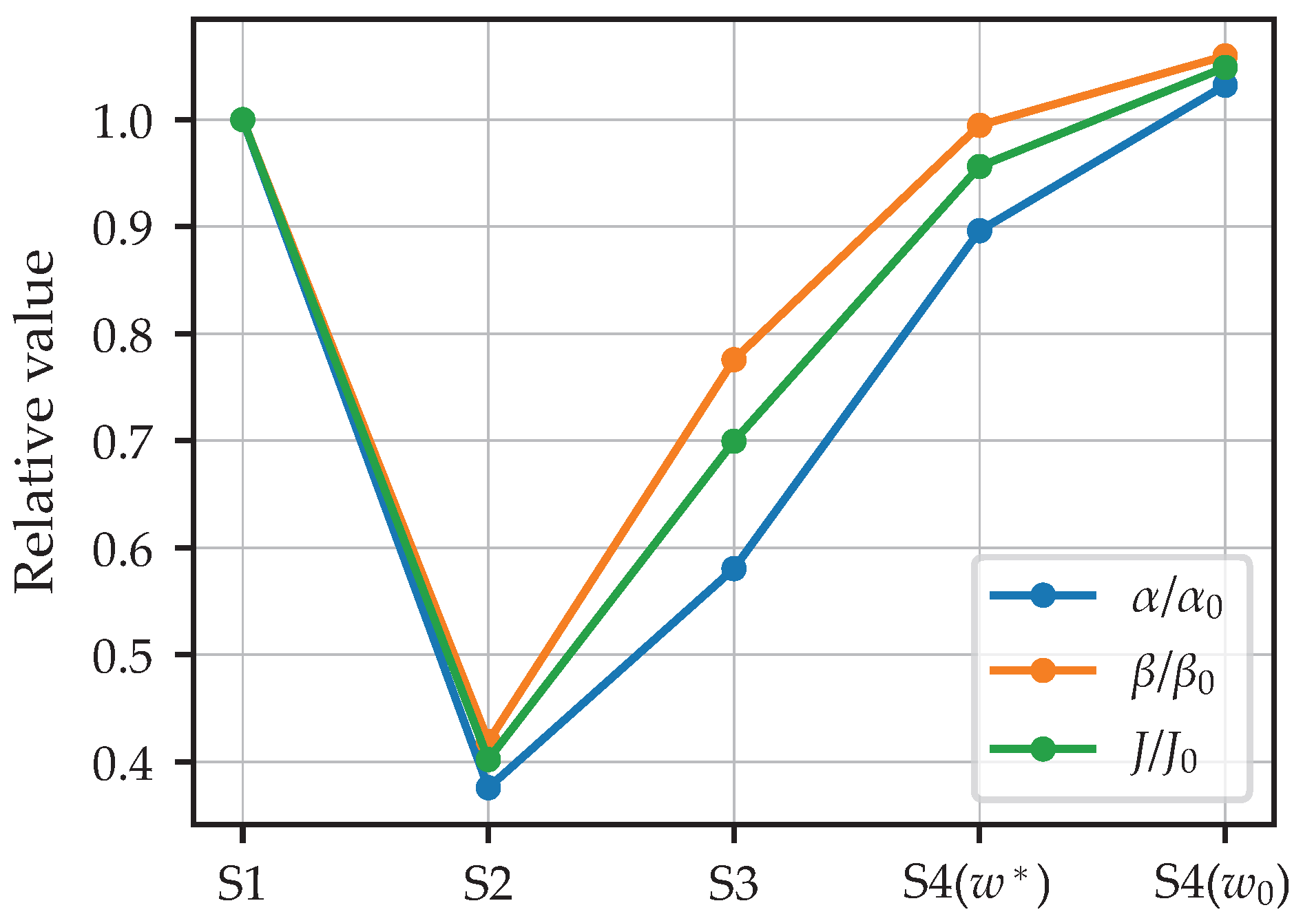
The computational experiment is organised as four Monte Carlo series. The reported series address baseline thresholding, repeated-measurement averaging, within-path confirmation, and measurement-level multi-fidelity fusion. In all reported series, solution quality is evaluated via unconditional CRIs ${\widehat{P}}_{\mathrm{TN},i}$, ${\widehat{P}}_{\mathrm{TP},i}$, ${\widehat{P}}_{\mathrm{FA},i}$, and ${\widehat{P}}_{\mathrm{MD},i}$ (Section 3.3), together with the corresponding conditional risks $\alpha$ and $\beta$ (Equations (6) and (7)) and the selected comparison criterion (e.g., $J_{\mathrm{err},\mathrm{raw}}$).

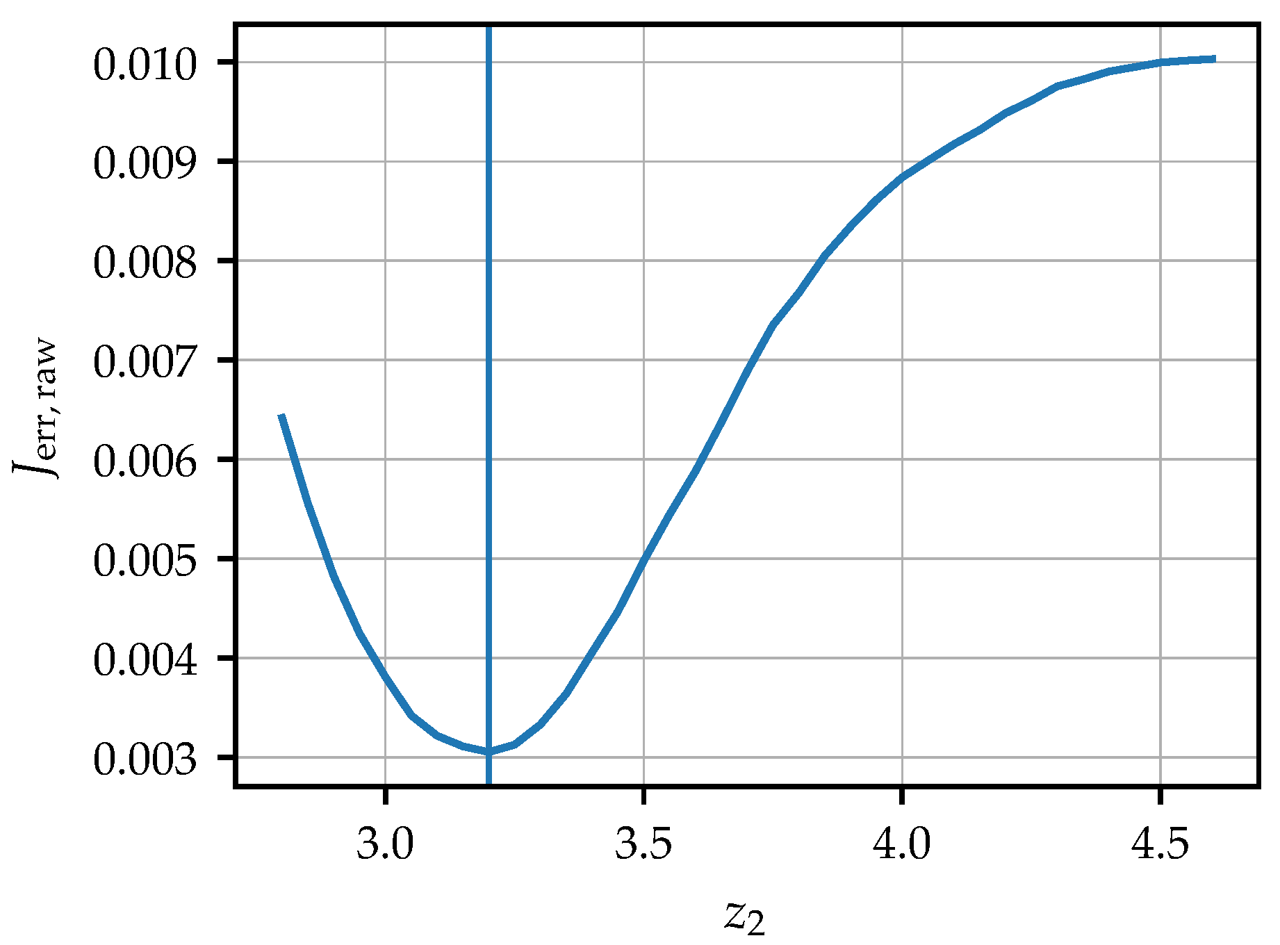
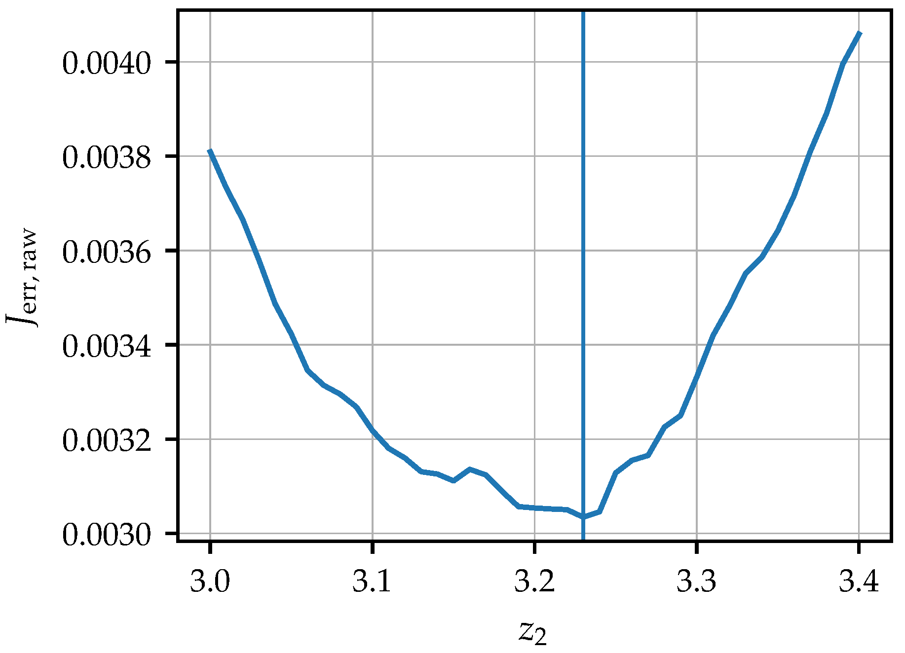
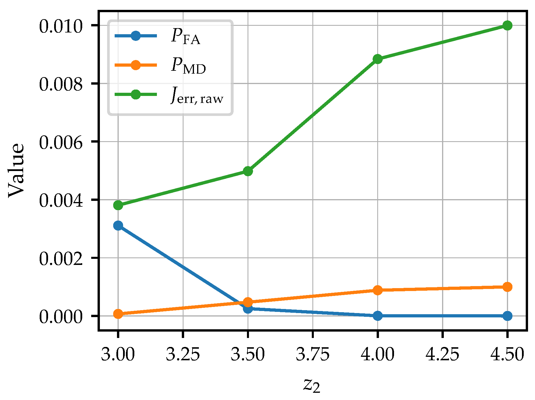
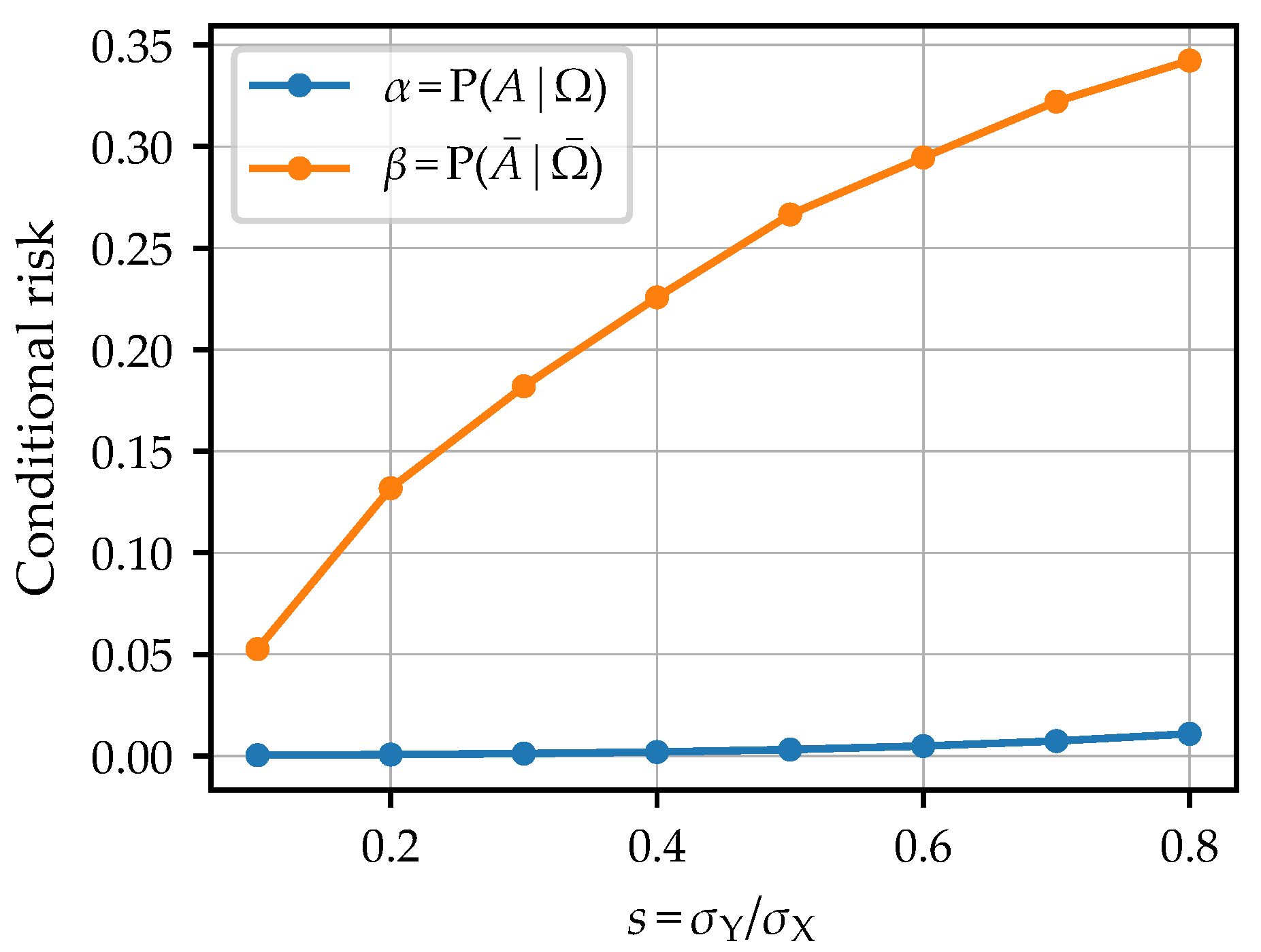
Series 1 (baseline threshold logic): (i) calibrate the baseline threshold formulation for the prescribed abnormal-state prior ${\pi }_{\mathrm{dev}}$ (normal-region bound set via ${\pi }_{\mathrm{dev}}\Rightarrow z_1$); (ii) select the optimal decision bound $z_2^{*}$ for fixed measurement-path accuracy; and (iii) assess sensitivity to s and the $P_{\mathrm{FA}}$–$P_{\mathrm{MD}}$ trade-off as functions of $z_2$.

Series 2 (within-cycle averaging): quantify the effect of averaging repeated measurements (representative point $n=5$) using the fixed thresholds obtained in Series 1.

Series 3 (within-path confirmation): assess the effect of “a out of m” confirmation over repeated cycles. Here, the setting $(a,m)=(2,3)$ is used as an illustrative reference case for comparison rather than as a universally optimal confirmation policy. For shipboard application, confirmation parameters should be linked to the sampling interval, the confirmation window, and the expected time scale of fault evolution.

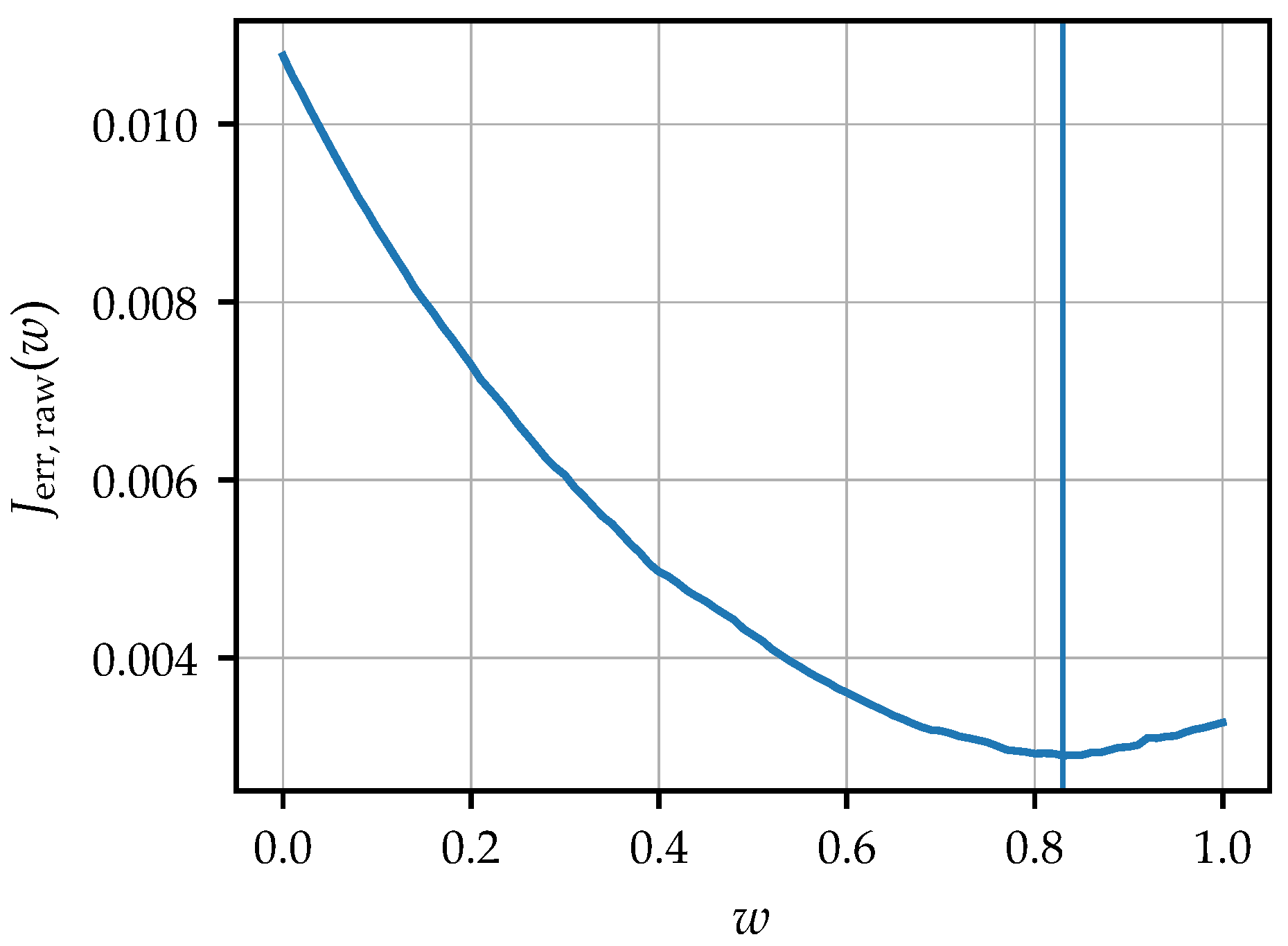
Series 4 (multi-fidelity fusion): assess the effect of two-path multi-fidelity fusion using a measurement-level combination with a fixed fusion weight. In this series, the weight w is optimised within a controlled setting and treated as a constant across the operating profile in order to isolate the contribution of multi-fidelity fusion. This formulation is intended for comparative analysis rather than as a final weighting policy for practical shipboard use.

The series parameters, fixed settings of ${\theta }_i$ (Equation (18)), and the controlled outputs are summarized in

Table 3. Computational experiment series plan (Monte Carlo verification protocol for decision logic using unconditional control-reliability indicators (CRIs)).

Series	Verified Decision-Logic Element	Fixed ${\mathit{\theta }}_{\mathit{i}}$ (Equation (18))	Varied Factors (Reported Simulation)	Model Relations Used	Controlled Outputs
1	Baseline single-path threshold decision (no repeats)	$M_i=1$, $n_{i1}=1$, $m_{i1}=1$, $K_i=1$; $a_i=b_i=c_i=1$. Normal bound set via ${\pi }_{\mathrm{dev}}\Rightarrow z_1$.	1.1: $z_2$ (search for $z_2^{*}$) at fixed $s=s_{\mathrm{fixed}}=0.3$ and fixed $z_1$. 1.2: $s\in \{0.1,\dots ,0.8\}$ at fixed $(z_1,z_2^{*})$. 1.3: control grid $z_2\in \{3.0,3.5,4.0,4.5\}$ at fixed $s_{\mathrm{fixed}}$.	Observation model (Equation (1)); regions $\Omega$ and $\omega$ (Equations (2) and (3)); CRI estimation (Equation (5)); risks $\alpha ,\beta$ (Equations (6) and (7)); $J_{\mathrm{err},\mathrm{raw}}$ (Appendix B.2, Appendix B.4).	${\widehat{P}}_{\mathrm{TN},i}$, ${\widehat{P}}_{\mathrm{TP},i}$, ${\widehat{P}}_{\mathrm{FA},i}$, ${\widehat{P}}_{\mathrm{MD},i}$; $\alpha$, $\beta$; $J_{\mathrm{err},\mathrm{raw}}$; dependencies on $z_2$ and s.
2	Repeated measurements and averaging $\overline{Z}$ within a path	$M_i=1$, $m_{i1}=1$, $K_i=1$; $n_{i1}=n$; $a_i=b_i=c_i=1$. Reported point: $n=5$.	No sweep: one point $n=5$ at $s_{\mathrm{fixed}}=0.3$ and fixed $(z_1,z_2^{*})$.	Equations (21)–(23); implementation uses the equivalent ${\sigma }_Y/\sqrt{n}$ representation for acceleration (Appendix B.5).	Same ${\widehat{P}}_{·,i}$, $\alpha$, $\beta$, $J_{\mathrm{err},\mathrm{raw}}$; comparison with Series 1.
3	Within-path confirmation (“a out of m”) over sub-cycles	$M_i=1$, $n_{i1}=1$, $m_{i1}=m$, $K_i=1$; $a_i=a$; $b_i=c_i=1$. Reported point: $(a,m)=(2,3)$.	No sweep: one point $(a,m)=(2,3)$ at $s_{\mathrm{fixed}}=0.3$ and fixed $(z_1,z_2^{*})$.	Primary decision (Equation (23)) with $n=1$; confirmation (Equation (24)); CRI estimation (Equation (5)); risks $\alpha ,\beta$ (Equations (6) and (7)).	Same ${\widehat{P}}_{·,i}$, $\alpha$, $\beta$, $J_{\mathrm{err},\mathrm{raw}}$; comparison with Series 1.
4	Two-path multi-fidelity measurement-level fusion ($M_i=2$)	$M_i=2$; $n_{i1}=n_{i2}=1$, $m_{i1}=m_{i2}=1$, $K_i=1$; $a_i=b_i=c_i=1$. Reported point: $(s_{i1},s_{i2})=(0.3,0.7)$.	$w\in [0,1]$ with step $0.01$ for selecting $w^{*}$ by minimizing $J_{\mathrm{err},\mathrm{raw}}$; the reference point $w_0=0.7$ is also evaluated.	Model (Equation (1)); measurement-level fusion (Equation (26)) in the special case $M_i=2$, $m_{ij}=1$; CRI estimation (Equation (5)); risks $\alpha ,\beta$ (Equations (6) and (7)); $J_{\mathrm{err},\mathrm{raw}}$ (Appendix B.7).	Same ${\widehat{P}}_{·,i}$, $\alpha$, $\beta$, $J_{\mathrm{err},\mathrm{raw}}$; $J_{\mathrm{err},\mathrm{raw}}\left(w\right)$; comparison of $w^{*}$ and $w_0$.

Note: the reported series quantify selected decision-logic elements within the proposed multi-stage framework; Stage 0 (data-quality gating) and Stage 5 (temporal filtering) are included in the architecture but are not separately isolated as standalone Monte Carlo series here. Detailed verbal descriptions of the series algorithms are provided in Appendix B; the Python implementation is included in the Supplementary Materials.

.

The reported series should be interpreted as control-point comparisons within a unified verification framework rather than as a full optimisation over the decision-logic design space. Accordingly, the reported gains quantify the behaviour of selected logic elements at representative points, not universal optimal settings for shipboard deployment.

4. Results

The results reported below correspond to the four Monte Carlo series introduced in Section 3.5. In all reported series, we used the same baseline setup (Section 3): X and Y were normally distributed; the regions were symmetric, $\Omega =[-z_1{\sigma }_X,z_1{\sigma }_X]$ and $\omega =[Z_L,Z_U]$ with $Z_L=-z_2{\sigma }_X$ and $Z_U=z_2{\sigma }_X$; and ${\sigma }_X=1$ with a fixed rarity parameter ${\pi }_{\mathrm{dev}}=0.001$. This stylized $Z=X+Y$ uncertainty model is used as a surrogate for ML-derived diagnostic statistics in PdM: X represents the latent health-related component of the statistic, whereas Y aggregates sensor and model-induced uncertainty that drives spurious threshold crossings and missed detections in practice. All results reported below are based on $N=2,000,000$ Monte Carlo trials, which yields small estimation error even for probabilities on the order of ${10}^{-4}$ (for $p\sim {10}^{-4}$, the standard error is on the order of ${10}^{-5}$). Therefore, between-series differences at the level of ${10}^{-4}$–${10}^{-3}$ are interpretable.

4.1. Series 1: Threshold Calibration and Decision-Region Selection (Baseline Single-Cycle Channel)

Calibration using a prescribed abnormal-state prior was performed by setting the scenario parameter ${\pi }_{\mathrm{dev}}=0.001$, which in this simulation corresponds to $z_1=3.290527$ and an empirical fraction of normal realizations close to the target $1-{\pi }_{\mathrm{dev}}=0.999$. This parameter is used to represent an extreme imbalance regime for controlled comparison of decision-logic variants, rather than as a direct engineering estimate of the actual failure rate of marine diesel engines.

Next, for a fixed noise ratio $s={\sigma }_Y/{\sigma }_X=0.3$, we selected the decision-region width parameter $z_2$ by minimizing the raw error criterion $J_{\mathrm{err},\mathrm{raw}}$. In this simulation, we used

$$J_{\mathrm{err},\mathrm{raw}}=P_{\mathrm{FA}}+10P_{\mathrm{MD}},$$

(28)

which prioritizes missed detections relative to false alarms.

A coarse grid search followed by local refinement yielded $z_2^{\left(\mathrm{coarse}\right)}=3.20$ and $z_2^{*}=3.23$ as the minimizer of $J_{\mathrm{err},\mathrm{raw}}$.

The key interpretation of $z_2^{*}$ is as follows. When $z_2<z_1$, the no-alarm region $\omega$ is narrower than the true normal region $\Omega$, so the channel becomes more conservative (it raises an alarm earlier). This reflects the adopted weighting in $J_{\mathrm{err},\mathrm{raw}}$: narrowing $\omega$ reduces $P_{\mathrm{MD}}$ and $\beta$ but increases $P_{\mathrm{FA}}$ and $\alpha$. The optimum $z_2^{*}$ fixes the resulting trade-off for the chosen weights. The coarse search and local refinement of $z_2^{*}$ are shown in Figure 1 and Figure 2, and the $P_{\mathrm{FA}}$–$P_{\mathrm{MD}}$ trade-off as a function of $z_2$ is shown in Figure 3.

For the selected baseline point (Series 1, $s=0.3$, $z_1=3.290527$, $z_2^{*}=3.23$), we obtained $P_{\mathrm{FA}}=0.0011845$, $P_{\mathrm{MD}}=0.0001850$, $\alpha =0.001186$, $\beta =0.181997$, and $J_{\mathrm{err},\mathrm{raw}}=0.0030345$. Under extremely rare abnormalities ($\sim 0.1\%$), the unconditional missed-detection probability $P_{\mathrm{MD}}$ remains small (on the order of ${10}^{-4}$); however, the conditional missed-detection risk given an abnormal state, $\beta$, is substantial (about $0.182$) in the baseline single-cycle scheme.

4.2. Series 1 (Continued): Sensitivity of Conditional Risks to the Noise Ratio

With fixed $z_1$ and $z_2^{*}$, we evaluated a grid of $s\in \{0.1,\dots ,0.8\}$. Both conditional risks increase as relative measurement accuracy deteriorates, with a markedly stronger increase in $\beta$ than in $\alpha$. At $s=0.1$, we obtained $\alpha \approx 3.72\times {10}^{-4}$ and $\beta \approx 0.0526$, whereas at $s=0.8$ we obtained $\alpha \approx 0.0109$ and $\beta \approx 0.3424$. Thus, as measurement-error variance increases relative to the variability of X, the channel rapidly loses sensitivity to rare abnormalities (i.e., $\beta$ increases). Methodologically, this supports the need for multi-stage decision logic (repeats, confirmation, and multi-fidelity), rather than reliance on a single threshold trigger. The dependencies $\alpha \left(s\right)$ and $\beta \left(s\right)$ are shown in Figure 4.

4.3. Series 2: Effect of Averaging Repeated Measurements

In Series 2, for the reference configuration $n=5$, we obtained $P_{\mathrm{FA}}=0.0004450$, $P_{\mathrm{MD}}=7.75\times {10}^{-5}$, $\alpha =0.000445$, $\beta =0.076242$, and $J_{\mathrm{err},\mathrm{raw}}=0.0012200$.

Relative to the baseline Series 1, this corresponds to:

• A $62.43\%$ reduction in $\alpha$ (ratio $0.376$);
• A $58.11\%$ reduction in $\beta$ (ratio $0.419$);
• A $59.80\%$ reduction in $J_{\mathrm{err},\mathrm{raw}}$ (ratio $0.402$).

From an engineering perspective, averaging five independent measurements substantially increases the robustness of the threshold decision against the random component Y and provides the largest gain among the methods evaluated at this point. In particular, it reduces both the false-alarm rate and the probability of missing a rare abnormality.

4.4. Series 3: Effect of “2 out of 3” Confirmation

Series 3 evaluates within-path confirmation at the illustrative reference case $(a,m)=(2,3)$ under the same baseline conditions used for Series 1. This setting is introduced here as a representative comparison case rather than as a universally optimal confirmation rule because a principled choice of a and m should depend on the sampling interval, the length of the confirmation window, and the expected time scale of fault evolution in the monitored object. At this point, we obtained $P_{\mathrm{FA}}=0.0006885$, $P_{\mathrm{MD}}=1.435\times {10}^{-4}$, $\alpha =0.000689$, $\beta =0.141171$, and $J_{\mathrm{err},\mathrm{raw}}=0.0021235$.

Relative to the baseline Series 1:

• $\alpha$ decreased by 41.89% (ratio 0.581);
• $\beta$ decreased by 22.43% (ratio 0.776);
• $J_{\mathrm{err},\mathrm{raw}}$ decreased by 30.02% (ratio 0.700).

Confirmation based on binary outcomes reduces both types of errors (false alarms and missed detections), but in this setup it is less effective than averaging (Series 2). This is expected because Series 3 operates after information loss due to binarisation (decisions $A/\overline{A}$ rather than a continuous Z).

4.5. Series 4: Multi-Fidelity Two-Path Fusion and Weight Optimization

Series 4 considers a controlled two-path multi-fidelity setting in which measurement-level fusion is implemented with a fixed weight across the operating profile. This fixed-weight formulation is used here as a deliberate simplification for comparing fusion against other decision-logic mechanisms, rather than as a general deployment policy. Within this setting, the optimisation yielded $w^{*}=0.83$. At this point, we obtained $P_{\mathrm{FA}}=0.0010615$, $P_{\mathrm{MD}}=0.0001840$, $\alpha =0.001063$, $\beta =0.181013$, and $J_{\mathrm{err},\mathrm{raw}}=0.0029015$.

The engineering reference weight $w_0=0.70$ yielded $J_{\mathrm{err},\mathrm{raw}}=0.0031825$, which is slightly worse than the baseline Series 1 ($J_{\mathrm{err},\mathrm{raw}}=0.0030345$). Moving from $w_0$ to $w^{*}$ improves $J_{\mathrm{err},\mathrm{raw}}$ by approximately $8.83\%$ within Series 4. The objective landscape and the selected optimum $w^{*}$ are shown in Figure 5.

4.6. Summary Comparison of Series (Control Point) and Implications for Multi-Stage Synthesis

To ensure a fair comparison, all variants are evaluated under the same baseline configuration with identical $z_1$ and $z_2^{*}$; therefore, differences are driven only by the logic component (averaging, confirmation, or multi-fidelity fusion). The results are summarized in

Table 4. Summary results at the shared baseline configuration for Series 1–4 (fixed $z_1=3.290527$, $z_2^{*}=3.23$; for Series 4 additionally $s_{i1}=0.3$ and $s_{i2}=0.7$).

Series	${\mathit{P}}_{\mathbf{TN}}$	${\mathit{P}}_{\mathbf{FA}}$	${\mathit{P}}_{\mathbf{TP}}$	${\mathit{P}}_{\mathbf{MD}}$	$\mathit{\alpha }$	$\mathit{\beta }$	${\mathbf{n}}_{\mathbf{norm}}$	${\mathbf{n}}_{\mathbf{dev}}$	${\mathbf{J}}_{\mathbf{err},\mathbf{raw}}$
Series 1	0.99780	0.00118	0.00083	0.00019	0.00119	0.18200	1,997,967	2033	0.00303
Series 2	0.99854	0.00045	0.00094	0.00008	0.00045	0.07624	1,997,967	2033	0.00122
Series 3	0.99830	0.00069	0.00087	0.00014	0.00069	0.14117	1,997,967	2033	0.00212
Series 4 ($w^{*}$)	0.99792	0.00106	0.00083	0.00018	0.00106	0.18101	1,997,967	2033	0.00290
Series 4 ($w_0$)	0.99776	0.00122	0.00082	0.00020	0.00122	0.19282	1,997,967	2033	0.00318

and Figure 6. Here, $n_{\mathrm{norm}}$ and $n_{\mathrm{dev}}$ denote the Monte Carlo counts of realizations with $X\in \Omega$ and $X\in \overline{\Omega }$, respectively (identical across Series 1–4 because $F\left(X\right)$ is fixed).

From the summary plot and Table 4, the following points can be concluded:

1.

The largest gain under the shared baseline configuration is achieved by averaging (Series 2): $\alpha$ decreases by a factor of ≈2.66, $\beta$ by a factor of ≈2.39, and $J_{\mathrm{err},\mathrm{raw}}$ by a factor of ≈2.49 relative to the baseline threshold decision.

2.

“2 out of 3” confirmation (Series 3) yields a consistent improvement, but weaker than averaging: $J_{\mathrm{err},\mathrm{raw}}$ decreases by about 30%, and $\beta$ by about 22% relative to Series 1.

3.

Multi-fidelity fusion (Series 4) with $s_{i1}=0.3$ and $s_{i2}=0.7$ provides only a small improvement over Series 1 when the weight is optimised ($w^{*}=0.83$): $J_{\mathrm{err},\mathrm{raw}}$ decreases by ≈4.4%, while $\beta$ remains nearly unchanged. Without optimisation (the reference point $w_0=0.70$), performance degrades slightly relative to Series 1.

Under the shared baseline configuration, averaging reduced both $\alpha$ and $\beta$ more strongly than “2 out of 3” confirmation, whereas two-path fusion provided only a limited gain after calibration of w. In other words, the compared mechanisms shift the $P_{\mathrm{FA}}$–$P_{\mathrm{MD}}$ trade-off in quantitatively different ways even under the same baseline threshold $z_2^{*}$.

5. Discussion

5.1. Interpretation of the Results

We evaluate decision-logic quality not by “classifier accuracy” but by probabilistic risks of false alarms and missed detections, defined through the unconditional control-reliability indicators $P_{\mathrm{TN}}$, $P_{\mathrm{TP}}$, $P_{\mathrm{FA}}$, and $P_{\mathrm{MD}}$, and the corresponding conditional risks.

Under extremely rare abnormal states, ${\pi }_{\mathrm{dev}}=0.001$ (i.e., $\mathrm{P}\left(\overline{\Omega }\right)\approx {10}^{-3}$), the unconditional missed-detection probability $P_{\mathrm{MD}}$ is inevitably small in magnitude. Here, ${\pi }_{\mathrm{dev}}=0.001$ is treated as a scenario parameter of the simulation. Within rare-abnormality settings of this kind, however, the conditional risk $\beta$ becomes especially informative, because it quantifies the probability of failing to detect an abnormality given that it is truly present. This is observed at the Series 1 reference setting: for $s={\sigma }_Y/{\sigma }_X=0.3$ and the error-optimal threshold $z_2^{*}=3.23$, we obtained $\beta \approx 0.182$. Thus, in the single-cycle threshold scheme, roughly one out of five to six abnormal cases does not trigger an alarm, indicating limited sensitivity to rare events at the given measurement-path accuracy.

Series 2 (within-path averaging of repeated measurements, $n=5$) provided the largest gain at the reference setting among the evaluated mechanisms: both $\alpha$ and $\beta$ decreased simultaneously (in particular, $\alpha$ decreased by approximately a factor of $2.66$ and $\beta$ by approximately a factor of $2.39$ compared to the baseline Series 1). At the common comparison point, the $n=5$ averaging scheme reduced $\alpha$ from $0.001186$ to $0.000445$ and $\beta$ from $0.182$ to $0.076$. This indicates that aggregation of the continuous quantity Z prior to binarisation suppresses the random component of the error Y more effectively than the other mechanisms compared at this setting.

Series 3 (confirmation over repeated cycles using a “2 out of 3” rule) also improves the indicators consistently (both $\alpha$ and $\beta$ decrease relative to Series 1), but it is less effective than averaging. A plausible explanation is information loss due to binarisation: Series 3 operates on discrete outcomes $A/\overline{A}$, whereas Series 2 aggregates continuous values Z before applying the threshold decision. At the reported control point, mechanisms operating before binarisation appear more effective than those applied after binarisation because they retain information carried by the continuous statistic Z. This observation should be interpreted as a result of the adopted surrogate setting and comparison protocol; confirming its generality requires broader parameter sweeps and validation on operational data.

Series 4 (multi-fidelity, two paths with $s_{i1}=0.3$ and $s_{i2}=0.7$, fused at the measurement level) reveals an important effect: adding a coarse measurement path does not guarantee improvement unless fusion parameters are tuned appropriately. Weight optimisation in the measurement-level fusion ${\overline{Z}}_i^{\left(k\right)}=w{\overline{Z}}_{i1}^{\left(k\right)}+(1-w){\overline{Z}}_{i2}^{\left(k\right)}$ (Equation (26); in Series 4, $n_{ij}=m_{ij}=1$ so ${\overline{Z}}_{ij}^{\left(k\right)}\equiv Z_{ij}^{(k,1,1)}$) yielded $w^{*}=0.83$, implying dominance of the more accurate path; with the engineering reference weight $w_0=0.70$, performance slightly degraded relative to the baseline Series 1, whereas the optimised weight yielded a small but consistent improvement in $J_{\mathrm{err},\mathrm{raw}}$. Thus, multi-fidelity design should be treated not as an automatic performance gain, but as a mechanism whose weights or voting rules require calibration.

5.2. Comparison with the Literature

Compared with the literature, the distinctive feature of the present study is not the use of thresholds, confirmation, or fusion as such, but their treatment as explicit, calibratable components of a channel-level decision logic evaluated under a common CRI-based protocol. In many applied marine studies, these elements are embedded implicitly in a model pipeline or heuristic warning scheme; here, they are isolated as design variables and compared on the same probabilistic basis.

Many applied studies on marine CBM/PdM specify the AD–FD structure and discuss deployment constraints, but the decision layer is often reduced to a single threshold on an anomaly score or residual without an explicit link to controlled risks such as $\alpha$ and $\beta$. In the reported baseline configuration ($z_2^{*}=3.23$, $s=0.3$), this distinction is visible: although unconditional $P_{\mathrm{MD}}$ is small, the conditional missed-detection risk remains $\beta \approx 0.182$. Rule-based and zone-based approaches are practically interpretable because they connect diagnostics to maintenance actions; however, zone boundaries are most often defined heuristically and are rarely quantified via error probabilities [56]. Residual-based approaches also motivate confirmation over observation sequences and explicit use of alarm history [57]. In the present formulation, the decision region $\omega$, confirmation parameters, and fusion rule are treated as explicit components of channel logic and compared through the same set of CRIs.

5.3. Study Limitations and Threats to Validity

1.

Distributional assumptions. The computational experiment uses normal distributions for X and Y and symmetric regions $\Omega$ and $\omega$. Real operational data may exhibit asymmetry, heavy tails, outliers, and nonstationarity. Therefore, the reported quantitative gains (in percent) should be interpreted within the adopted uncertainty model; for real data, the robustness of the conclusions should be verified under more realistic distributions for $F\left(X\right)$ and $F\left(Y\right)$.

2.

Interpretation of the rarity parameter. The value ${\pi }_{\mathrm{dev}}=0.001$ is introduced in this paper as a scenario parameter for studying the decision logic under extreme class imbalance. It is not calibrated here against fleet-level maintenance data or failure statistics for marine diesel engines. Therefore, conclusions related to rarity should be interpreted within the adopted simulation setting, whereas deployment-oriented calibration would require maintenance logs, fleet statistics, or domain-specific abnormality priors.

3.

Independence of repeats. The averaging effect (Series 2) assumes that the noise component across repeated measurements is largely uncorrelated. Under strong autocorrelation (sensor drift, slow operating-condition fluctuations, or process inertia), the effective variance reduction will be smaller. In such cases, it may be necessary to increase the interval between measurements, use robust aggregation, or combine averaging with confirmation over cycles.

4.

Operating-condition heterogeneity. In real operation, the distribution of X is a mixture over operating conditions (load, speed, and thermal conditions), and the error Y may also depend on operating conditions. Consequently, transferring thresholds and confirmation parameters requires operating-condition normalisation (or a residual-based formulation relative to expected normal behaviour under a given operating condition) and calibration of $\omega$ as a function of operating conditions.

5.

Confirmation-parameter selection. In this study, the setting $(a,m)=(2, 3)$ is used as an illustrative reference case for comparing confirmation against other decision-logic mechanisms. This choice is not sufficient to support a general design recommendation. For shipboard application, confirmation parameters should be linked to the sampling interval, the observation window, and the characteristic time scale of abnormality development. Generalisable recommendations therefore require either a parameter sweep over $(a,m)$ or calibration against operational data and domain-specific dynamics.

6.

Multi-fidelity monitoring and correlated path errors. Series 4 considers a specific scenario with two measurement paths and linear measurement-level fusion using a fixed weight across the operating profile. In practice, however, path reliability may vary with operating conditions, and errors across measurement paths may be correlated because of shared disturbance sources, common calibration drift, or synchronization effects. Under such conditions, a single global weight may be insufficient for deployment-oriented decision logic. More general recommendations therefore require parameterization over path accuracies, correlation structure, and regime-dependent weighting policies.

7.

Monte Carlo accuracy. With $N=2\times {10}^6$, the estimation accuracy is sufficient for probabilities on the order of ${10}^{-4}$–${10}^{-3}$ and for comparing series under the shared baseline configuration. For more stringent target levels (e.g., $P_{\mathrm{MD}}\sim {10}^{-6}$), either larger N or variance-reduction techniques would be required, together with checks of reproducibility and stability of random number generation.

5.4. Practical Integration of CBM Logic into CMMS/EAM and Requirements for Measurement and Computation

For shipboard implementation, the Stages 0–5 logic may be mapped onto a CMMS/EAM workflow by logging a minimal, traceable set of decision attributes for each monitored channel (e.g., the admitted-path flags $g_{ij}^{\left(k\right)}$, the effective window size $|{\mathcal{K}}_i|$, and the outcomes of within-path confirmation and $K_i$-cycle filtering). This makes each alarm/no-alarm outcome ${\overline{A}}_i/A_i$ auditable in terms of which paths participated and which rule confirmed (or rejected) the event.

A maintenance trigger can then be defined in terms of a confirmed event (e.g., after “a out of m” confirmation and/or “c out of K” filtering) rather than a single threshold crossing. In this study, mechanisms that act before binarisation (e.g., averaging in Series 2) reduced both $\alpha$ and $\beta$ more strongly than confirmation alone. Whether the same prioritisation holds in deployment depends on the sampling interval, operating-profile variability, and data quality, and should be verified on operational data.

One plausible architecture is to run data-quality gating, computation of diagnostic statistics, and confirmation/filtering onboard (edge), while performing periodic recalibration of thresholds and fusion weights offline using accumulated data and maintenance logs. The feasibility of this split depends on the available computing budget and connectivity constraints.

Computational budget and scalability should also be considered when the proposed CRI-based calibration is used in practice. In the supplementary implementation, a full Monte Carlo run for Series 1–4 with $N=2\times {10}^6$ required about 5.8 s of wall-clock time on a 12th Gen Intel Core i5-12500H system with 16 GB RAM (Python 3.13.13, NumPy 2.3.3). Peak memory usage remained below 1 GB (about 0.34 GiB working set and 0.82 GiB private memory). Because the threshold and weight sweeps use fixed grids, the computational cost is governed mainly by the Monte Carlo sample size and scales approximately linearly with N. This supports periodic recalibration as an offline engineering task after operating-profile updates; onboard operation can then use fixed pre-calibrated parameters in real time.

5.5. Directions for Future Research

Further work should extend the control-point comparisons reported here (e.g., $n=5$, $(a,m)=(2, 3)$, and two-path fusion with $w^{*}=0.83$) to broader parameter grids over $(s,{\pi }_{\mathrm{dev}})$ and $(n_{ij},m_{ij},a_i,b_i,K_i,c_i)$ and, where relevant, over the number of active paths $M_i$. Such computations would enable linking design choices to sampling intervals, confirmation-window duration, expected fault-evolution time scales, and time/cost constraints. A related step is to replace the scenario value of ${\pi }_{\mathrm{dev}}$ used here with priors derived from maintenance logs, fleet statistics, or domain-specific estimates of abnormality occurrence.

The uncertainty model should also be extended beyond the Gaussian stationary baseline to include outliers, drift, autocorrelation, mixtures of operating conditions in both $F\left(X\right)$ and $F\left(Y\right)$, missing data, correlated path errors, asynchronous sampling, and dynamically changing sets of active paths.

In addition, the framework should be validated on long-term operational data from physical marine diesel engines. This includes formation of the observable diagnostic quantity Z, operating-condition-dependent specification of the decision region $\omega$, calibration of confirmation parameters through CRIs using maintenance logs and expert-verified events, and evaluation of adaptive fusion policies instead of the fixed-weight scheme used in Series 4.

6. Conclusions

This study establishes a CRI-based framework for synthesising and comparing multi-stage CBM decision logic for marine diesel monitoring under rare abnormalities, measurement uncertainty, and heterogeneous channel quality. The key result is methodological: the paper treats implementable decision logic—not a single threshold or classifier output—as the primary design object and evaluates its variants through a unified Monte Carlo verification protocol.

Using a Monte Carlo computational experiment ($N=2\times {10}^6$) with ${\pi }_{\mathrm{dev}}=0.001$, we compared a baseline single-cycle threshold scheme with three reliability-enhancement mechanisms: averaging of repeated measurements, “a out of m” confirmation over repeated cycles, and two-path multi-fidelity measurement-level fusion. The baseline risks were $\alpha =0.001186$, $\beta \approx 0.182$, and $J_{\mathrm{err},\mathrm{raw}}=0.00303$. Averaging (Series 2, $n=5$) reduced them to $\alpha =0.000445$, $\beta =0.0762$, and $J_{\mathrm{err},\mathrm{raw}}=0.00122$, whereas confirmation (Series 3, $(a,m)=(2, 3)$) yielded $\alpha =0.000689$, $\beta =0.141$, and $J_{\mathrm{err},\mathrm{raw}}=0.00212$. Multi-fidelity monitoring (Series 4) improved performance only when fusion parameters were tuned appropriately: the optimal weight $w^{*}$ shifted toward the more accurate path, whereas non-optimal engineering weights yielded little or no gain under the adopted error criterion.

The practical significance of the framework lies in its compatibility with AD–FD architectures in which AI/ML modules generate the diagnostic statistic Z, while a downstream decision layer transforms this statistic into traceable maintenance triggers. In the present paper, this integration is demonstrated at the level of a Gaussian surrogate verification protocol; extending the framework to implementation-specific, operating-condition-dependent shipboard data remains the next necessary step.