Article

STID-Mixer: A Lightweight Spatio-Temporal Modeling Framework for AIS-Based Vessel Trajectory Prediction

1
School of Computer Science, Yangtze University, Jingzhou 434023, China
2
School of Computer Science and Engineering, Nanjing University of Science and Technology, Nanjing 210094, China
*
Author to whom correspondence should be addressed.
Eng 2025, 6(8), 184; https://doi.org/10.3390/eng6080184
Submission received: 24 June 2025 / Revised: 28 July 2025 / Accepted: 31 July 2025 / Published: 3 August 2025

Abstract

The Automatic Identification System (AIS) has become a key data source for ship behavior monitoring and maritime traffic management, widely used in trajectory prediction and anomaly detection. However, AIS data suffer from issues such as spatial sparsity, heterogeneous features, variable message formats, and irregular sampling intervals, while vessel trajectories are characterized by strong spatial–temporal dependencies. These factors pose significant challenges for efficient and accurate modeling. To address this issue, we propose a lightweight vessel trajectory prediction framework that integrates Spatial–Temporal Identity encoding with an MLP-Mixer architecture. The framework discretizes spatial and temporal features into structured IDs and uses dual MLP modules to model temporal dependencies and feature interactions without relying on convolution or attention mechanisms. Experiments on a large-scale real-world AIS dataset demonstrate that the proposed STID-Mixer achieves superior accuracy, training efficiency, and generalization capability compared to representative baseline models. The method offers a compact and deployable solution for large-scale maritime trajectory modeling.

1. Introduction

With the continuous expansion of global maritime transport, vessel behavior prediction has become increasingly critical in a wide range of applications, including maritime safety management, route optimization, and smart port operations. The Automatic Identification System (AIS), a core data source for modern maritime monitoring, broadcasts dynamic vessel information—such as position, speed over ground (SOG), course over ground (COG), and timestamps—through Very High Frequency (VHF) channels in real time [1,2,3]. According to incomplete statistics, AISs worldwide generate billions of messages per day. Extracting meaningful patterns from this vast data stream for high-quality trajectory prediction remains a pressing challenge in the maritime domain.
However, modeling AIS data introduce multiple challenges [4]. On one hand, AIS messages are highly irregular and heterogeneous: sampling frequencies are inconsistent, message types vary, and each message may contain different combinations of static and dynamic attributes. The feature structures are often complex and inconsistent, and some records suffer from missing values or erroneous reports, which significantly increases the cost of data processing and cleaning. On the other hand, vessel behavior exhibits strong spatial clustering and temporal dependencies. Trajectories are often sparse and discontinuous in geographic space and are subject to various sources of uncertainty, including weather conditions, shipping routes, and port operations [5]. These factors collectively lead to high complexity in trajectory modeling. While many existing methods are based on Recurrent Neural Networks (e.g., RNNs, LSTMs) or attention mechanisms (e.g., Transformers) [6,7,8,9,10], they often suffer from excessive parameters, high training costs, and slow inference speeds, limiting their suitability for deployment in real-time or large-scale scenarios [11,12,13]. Therefore, there is a clear need for a lightweight modeling framework that balances representational power with computational efficiency, particularly for handling massive AIS data.
To address these challenges, this paper proposes a trajectory prediction framework that integrates Spatial-Temporal Identity (STID) encoding with a Multi-Layer Perceptron Mixer (MLP-Mixer) architecture. The proposed approach first discretizes the target maritime region into a fixed grid and extracts periodic temporal features—such as hour of the day and day of the week—from each trajectory point, forming a unified spatio-temporal representation. The MLP-Mixer backbone is then employed to perform dual modeling in both the temporal and feature dimensions, capturing temporal dependencies and cross-feature interactions without relying on convolutional or attention-based mechanisms. The final prediction is framed as a classification task, where the model outputs the most likely grid cell that the vessel will occupy in the future. In this study, we aim to explore the theoretical feasibility of a lightweight modeling framework for vessel trajectory prediction based on AIS data. Our goal is to validate whether a pure MLP-based architecture, combined with structured spatio-temporal identity encoding, can achieve competitive performance while reducing model complexity. This work serves as a foundation for future efforts toward real-world deployment in large-scale maritime environments.
The main contributions of this study are as follows:
  • Lightweight prediction framework: We propose STID-Mixer, a compact yet expressive model tailored for AIS trajectory prediction. It eliminates the need for convolutional and attention-based mechanisms while preserving high accuracy and scalability.
  • Unified spatio-temporal representation: A joint embedding scheme encodes discrete temporal features (e.g., hour, weekday), spatial grid identifiers, and normalized continuous AIS attributes, enabling effective modeling of complex spatio-temporal vessel behaviors.
  • Improved predictive performance and efficiency: Extensive experiments show that STID-Mixer consistently outperforms several strong baselines (e.g., LSTM, Transformer, GBDT [14]) in terms of prediction accuracy, F1 score and training time.
  • Generalization and practical potential: The model demonstrates robust generalization on large-scale trajectory forecasting tasks, offering a deployable and adaptable solution for real-world maritime behavior modeling.

2. Related Work

In recent years, with the advancement of intelligent shipping and maritime traffic management technologies, AIS-based vessel trajectory prediction has attracted increasing attention [1,15]. Researchers have proposed a variety of modeling approaches to address the noisy, irregular, and highly spatiotemporal-dependent characteristics of AIS data [16]. The research landscape has evolved from early probabilistic models to deep learning-based structural optimization methods.
In the early stages, Ristic et al. (2008) pioneered the use of particle filtering for AIS trajectory modeling [17]. By leveraging state-space models, they dynamically estimated the future positions of vessels, laying the groundwork for probabilistic approaches in this domain. Pallotta et al. (2013) subsequently proposed the Trajectory Reconstruction and Evaluation for Anomaly Detection model (TREAD) [11], which clusters historical trajectories into standard route templates and applies probabilistic distributions for behavior prediction. Building on this, Mazzarella et al. (2015) introduced Bayesian networks for dynamic prediction, enhancing robustness in detecting anomalous vessel behaviors [4]. However, these early methods heavily relied on prior knowledge and trajectory matching strategies, making them less effective in handling the complex and evolving spatiotemporal patterns inherent in real-world AIS data. With the rapid development of deep learning, Recurrent Neural Networks (RNNs), known for their sequential modeling capabilities, became widely adopted [2,18,19,20]. Forti et al. (2020) proposed a sequence-to-sequence neural framework for AIS trajectory prediction using a Long Short-Term Memory (LSTM) encoder-decoder architecture [21]. This approach enables the generation of future vessel positions based on historical AIS observations, effectively capturing long-range temporal dependencies. However, such architectures are often constrained by sequential processing inefficiencies and limited scalability. To enhance structural modeling beyond single-sequence representations, some studies began exploring graph-based modeling paradigms. Shi et al. (2021) introduced the Sparse Graph Convolutional Network (SGCN) [22] for pedestrian trajectory prediction, which constructs sparse adjacency graphs to capture inter-trajectory relationships. This idea has inspired similar applications in AIS data, emphasizing structural interaction modeling. To address efficiency and modeling bottlenecks in traditional RNN architectures, Cheng et al. (2022) proposed a two-stage spatio-temporal Hybrid-GCGRU [23], integrating graph convolution with gated recurrent units to capture spatial topology and temporal dependencies in sparse trajectory data. This hybrid approach achieves notable improvements in heterogeneous feature representation and long-range sequence prediction accuracy, offering methodological inspiration for AIS trajectory modeling. Lin et al. (2023) proposed the TTCN-Attention-GRU model [24], which combines temporal convolutional networks with gated recurrent units and attention mechanisms to capture long-range temporal dependencies and improve prediction accuracy in AIS trajectory data. On the input representation side, Shao et al. (2022) proposed the Spatial-Temporal Identity (STID) [25] module, which encodes time and space into learnable embeddings. Although originally designed for multivariate time series (MTS) forecasting, this approach offers a compelling perspective for lightweight spatiotemporal representation learning in AIS applications. In parallel, lightweight and highly parallelizable architectures have garnered attention. Tolstikhin et al. (2021) introduced the MLP-Mixer architecture [26], which eliminates both attention mechanisms and convolutions by using pure multilayer perceptrons (MLPs) to model dependencies along spatial and channel dimensions. Initially applied in visual recognition tasks, MLP-Mixer has gradually been extended to sequence modeling and trajectory prediction, offering a new paradigm for efficient neural network design [27,28].
Over the past few years, the research on AIS trajectory prediction has evolved from rule-based and probabilistic models to deep learning-driven sequence modeling. Although RNNs are effective for sequential learning, their high computational cost and lack of parallelism limit scalability. Graph-based and attention-based models enhance the ability to model vessel interactions but often involve complex structures and high deployment costs [7]. However, few studies have examined the use of identity-based temporal encoding in combination with pure MLP architectures for vessel trajectory forecasting. Based on these advancements, this paper proposes a lightweight and efficient trajectory prediction framework by integrating the STID module with the MLP-Mixer method. Without relying on attention mechanisms, the proposed model enables joint spatiotemporal feature learning while achieving a strong balance between accuracy and inference efficiency, offering a promising solution for AIS-driven prediction at scale.

3. Materials and Methods

3.1. Training Settings

All experiments were conducted on a single NVIDIA GeForce RTX 3060 GPU (NVIDIA Corporation, Santa Clara, CA, USA) paired with an 11th Gen Intel (R) Core (TM) i7-11800H @ 2.30GHz processor (Intel Corporation, Santa Clara, CA, USA). The entire training pipeline was implemented using Python 3.10 and developed based on the PyTorch 1.13 deep learning framework.

3.2. AIS Data Cleaning and Preprocessing

While the AIS provides a rich data foundation for maritime traffic monitoring, the quality and structure of raw AIS data are often compromised due to complex maritime communication environments [2] and limitations in message broadcasting mechanisms. For example, AIS messages exhibit irregular sampling frequencies and heterogeneous formats, with significant variations in the fields carried by different message types. Additionally, issues such as missing fields, duplicate records, static noise, and abnormal drifts are frequently observed. These problems not only degrade the integrity of trajectory information but also significantly increase the complexity of downstream modeling.
To address these challenges, a systematic data cleaning and preprocessing pipeline was applied prior to model training. The workflow consists of the following four key steps:
  • Message Parsing: Raw AIS messages in NMEA 0183 format [29] were parsed to extract essential fields, including Maritime Mobile Service Identity (MMSI), timestamp, longitude, latitude, Speed Over Ground (SOG), and Course Over Ground (COG), which were then stored in structured formats.
  • Record-Level Filtering: Redundant or erroneous data were removed through filtering operations, including the elimination of duplicate records, invalid MMSI entries, and records with missing fields or invalid values (e.g., SOG = 0 and COG = 360), which typically indicate non-moving or unreliable observations.
  • Trajectory Structuring and Quality Control: At the trajectory level, segmentation was performed based on temporal intervals. Additionally, messages of irrelevant types were excluded, short trajectory segments were discarded, and overly long trajectories were split to ensure manageable sequence lengths for modeling.
  • High-Frequency Broadcast Merging: To mitigate the redundancy caused by high-frequency AIS broadcasts—particularly from certain message categories within short time windows—a compression strategy was implemented. Within a sliding window of 25 to 35 s, only the final record in each group of closely spaced messages was retained, effectively sparsifying the trajectory structure and reducing modeling overhead.
Following this multi-stage cleaning process, the retained dynamic features included MMSI, SOG, COG, longitude (LON), latitude (LAT), and timestamp (Time). To unify the scale of continuous variables and enhance model stability, all continuous features were normalized using Min–Max scaling, computed as follows:
x = x x m i n x m a x x m i n
where x is the original value, x is the normalized value, and x m a x x m i n represent the minimum and maximum values of the feature across the dataset. This approach compresses the values into the [0, 1] range while preserving relative differences, facilitating faster convergence and more stable optimization during model training.

3.3. Datasets

The AIS trajectory dataset used in this study consists of continuous dynamic information for multiple vessels operating within a specified maritime region. Each data record contains the vessel’s Maritime Mobile Service Identity (MMSI), relative timestamp (Time), hour of day (Hour), day of week (Weekday), longitude (LON), latitude (LAT), spatial grid index (Grid_id), speed over ground (SOG), course over ground (COG), and trajectory segment identifier (Traj_id).
The preprocessed dataset is stored in CSV format, with a total size of 2.09 GB, comprising 24,174,306 AIS message records. These messages capture continuous sailing trajectories of hundreds of vessels over several consecutive days, making the dataset both large-scale and representative for maritime behavior modeling. The AIS data used in this study were obtained from the South China Sea Navigation Service Center of the China Maritime Safety Administration. The data are classified and subject to confidentiality restrictions, requiring formal access authorization from relevant government authorities. All data were anonymized prior to analysis. Access to the AIS data can be requested through the official platform: China MSA AIS Service Platform [30].
To meet the structural and semantic requirements of the proposed prediction model, the raw AIS data were subjected to a series of cleaning, spatio-temporal encoding, and preprocessing procedures, as detailed in Section 3.2. An example of the structured trajectory samples constructed from the dataset is shown in Table 1.
To ensure fair model evaluation and maintain the integrity of trajectory sequences, this study adopts a trajectory-level partitioning strategy. Specifically, all trajectory segments are first assigned unique identifiers (traj_id), which are then divided into training, validation, and test sets according to a fixed ratio. The dataset is split such that 70% of the trajectories are used for training, and the remaining 15% each for validation and testing. This trajectory-based partitioning effectively prevents data leakage caused by overlapping trajectory fragments across different subsets, thereby enhancing the independence and reliability of performance evaluation.

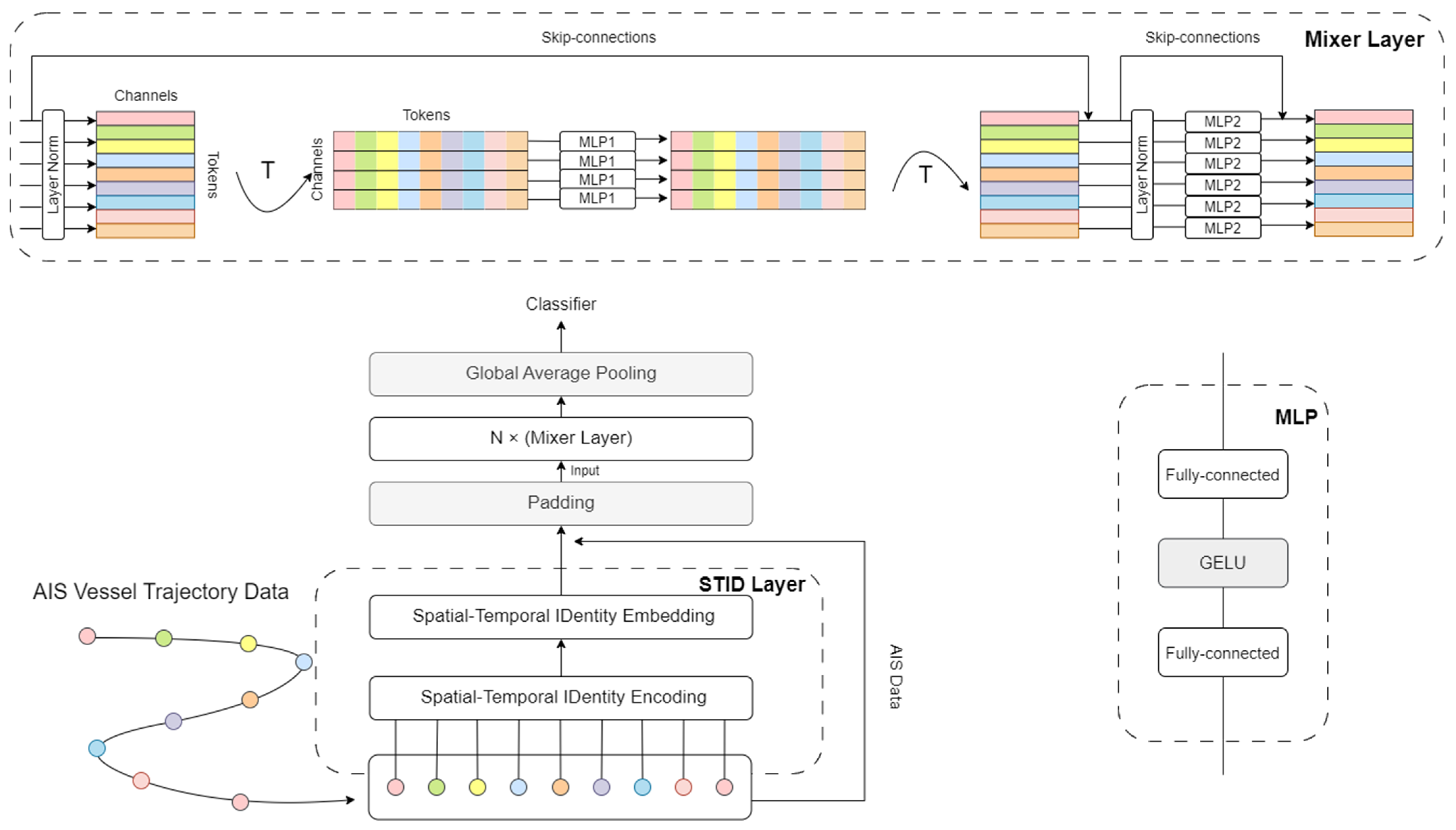
3.4. Model Architecture

Let a vessel’s AIS trajectory within a specific time interval be represented as a time-ordered sequence:
T   = x 1 , x 2 , , x n ,
where T denotes the trajectory sequences composed of n observed AIS points. Each trajectory point x i includes the timestamp, geographic coordinates (longitude and latitude), Speed Over Ground (SOG), and Course Over Ground (COG), along with other navigational features. The objective of this study is to predict the vessel’s most likely spatial location at a future time step, based on the preceding n 1 trajectory points in the sequence.
To improve both the practical utility and spatial interpretability of the prediction results, the maritime region is partitioned into a fixed 50 × 50 uniform grid. This grid resolution is determined based on the geographic extent and traffic characteristics of the target region. The studied area spans approximately 42 × 41 km2, located near a river estuary. Under this grid resolution, each cell covers approximately 0.84 × 0.82 km2, with a diagonal distance of around 1.17 km. Considering that the AIS sampling interval is roughly 30 s and that typical vessel speeds in this region range between 5 and 15 knots (≈2.5–7.7 m/s), the maximum displacement between consecutive observations is approximately 230 m. This indicates that, in most cases, vessels do not cross multiple grid cells within a single time step, nor do they remain within the same cell for extended periods.
Even when consecutive observations fall within the same cell, this often reflects real-world behaviors—such as anchoring, docking, or slow maneuvers near port areas. In addition, dynamic features such as Speed Over Ground (SOG), Course Over Ground (COG), hour, and weekday allow the model to differentiate between stationary and mobile states, improving its ability to learn complex vessel behavior patterns. Therefore, the 50 × 50 grid provides a practical balance between spatial resolution and label granularity, ensuring sufficient expressiveness without causing excessive class imbalance or over-sparsity.
Based on this spatial discretization, the trajectory prediction task is then formulated as a multi-class classification problem, where the model predicts the grid cell ID corresponding to the vessel’s future position. The input to the model is a sequential representation of historical trajectory features, and the output is the discrete grid cell index indicating the predicted location. Formally, the problem can be expressed as learning a prediction function f · , such that
y ^   =   f x 1 , x 2 , , x n 1 , y ^ 1,2 , , G
where G denotes the total number of grid cells in the discretized maritime space, each element x i is a feature vector comprising both normalized continuous variables (e.g., SOG, COG, LAT, LON and time) and embedded discrete temporal-spatial identifiers (e.g., hour, weekday, grid ID), and y ^ is the predicted grid ID. By reformulating vessel trajectory forecasting as a spatial classification task, the proposed approach enhances model deployability and facilitates integration into downstream visualization and decision-support systems.
To enable efficient modeling and prediction of future vessel behaviors, this study proposes a lightweight trajectory prediction framework, as illustrated in Figure 1. The framework begins with raw AIS trajectory data and proceeds through three key stages: spatio-temporal feature encoding and embedding, trajectory sequence modeling, and final classification-based prediction. The overall architecture is compact and computationally efficient, making it well-suited for large-scale maritime trajectory datasets.
Given that raw AIS data contain key attributes such as timestamps, geographic coordinates (LAT and LON), SOG, and COG, their physical characteristics are continuous and heterogeneous, making it difficult to directly capture the periodic behavior patterns and spatial aggregation of vessel movements. To address this, we introduce a spatio-temporal identity (STID) encoding mechanism. By discretizing continuous temporal and spatial features, the model transforms raw attributes into standardized categorical representations. On the temporal side, two typical periodic variables—hour of day (Hour) and day of week (Weekday)—are extracted from each timestamp to characterize the vessel’s intra-day and weekly behavior patterns. These variables are discretized into 24 and 7 categories, respectively. On the spatial side, the study area is divided into a 50 × 50 uniform grid, and each trajectory point is mapped to a unique Grid ID based on its latitude and longitude coordinates, serving as a discrete spatial identifier. Formally, for each timestamp t and position l o n , l a t , we define the spatio-temporal identity (STID) as follows:
S T I D = f h o u r t , f w e e k d a y t , f g r i d l o n , l a t
where f h o u r t denotes the hour of day extracted from timestamp t , ranging from 0 (0 AM) to 23 (11 PM); f w e e k d a y t denotes the day of the week, with values from 0 (Monday) to 6 (Sunday); f g r i d l o n , l a t maps the vessel’s coordinates to a grid cell ID within the predefined spatial grid (e.g., a 50 × 50 partitioning yields IDs from 0 to 2499).
Each categorical identifier—hour, weekday, and grid—is first represented as a discrete integer value f i , and then mapped to a learnable dense vector via its embedding matrix:
e i = E m b e d f i , i h o u r , w e e k d a y , g r i d
Through this mapping, each discrete ID is transformed into a fixed-length dense vector e i R d , where d denotes the embedding dimension. These embedding vectors provide semantic representations of temporal and spatial contexts, enabling the model to learn latent patterns associated with different time periods and geographical regions. In addition, since STID features are discrete and drawn from fixed value ranges, we experimented with several embedding dimensions during development. However, their impact on overall performance was minimal—especially compared to the continuous vessel features, which had a more pronounced influence on model behavior, as detailed in Section 4.1. Therefore, we use a fixed embedding dimension for all STID features in this study.
Together, these categorical features form the core of the STID encoding and are mapped to fixed-length vectors via their respective embedding matrices, enabling the model to capture structural patterns across temporal and spatial dimensions. Figure 2 illustrates the spatial grid partitioning and trajectory point encoding. A sample 5 × 5 region is shown, with vessel trajectory points projected onto corresponding grid cells and annotated with their respective Grid IDs. For visualization and privacy considerations, the latitude and longitude coordinates have been normalized to the [0, 1] range and do not reflect actual geographic location or specific units and values.
For the core model architecture, this study adopts an MLP-Mixer–based sequential representation approach, constructed by stacking multiple identical submodules. Unlike traditional architectures based on recurrent networks or attention mechanisms, the MLP-Mixer is fully built upon multi-layer perceptrons (MLPs) and operates independently across two dimensions. Before introducing the mathematical formulation, we first provide an intuitive overview. In the temporal dimension, the model first transposes the input trajectory sequence and then applies MLP transformations to enable information exchange across different time steps—this operation is referred to as token mixing. In the feature dimension, each trajectory point’s multi-dimensional attributes are fused through MLP layers, referred to as channel mixing, to enhance the local representational capacity. These two types of operations are alternated to capture both temporal dependencies and feature interactions in the sequence. Both submodules are equipped with layer normalization and residual connections, and use dropout regularization to mitigate overfitting, thereby improving both model expressiveness and training stability.
Formally, let the input to the MLP-Mixer block be a tensor X     R B × T × D , where B is the batch size, T is the number of time steps (tokens), and D is the feature dimension per token. Each MLP-Mixer layer consists of two main operations:
  • Token Mixing:
X   =   X   +   M L P t o k e n L a y e r N o r m X T T
This operation enables interaction between different time steps within a trajectory. Here, L a y e r N o r m ( X )     R B × T × D denotes layer normalization applied along the last dimension (feature-wise), which stabilizes training by standardizing each token’s feature vector. The transpose operator · T swaps the time and feature dimensions (i.e., T D ) so that the shared MLP operates across tokens (temporal positions). The result is then transposed back to the original shape. X     R B × T × D denotes the output of token mixing, retaining the original shape for subsequent processing.
  • Channel Mixing:
Y   =   X   +   M L P c h a n n e l L a y e r N o r m X
This stage fuses feature-wise interactions across each token. The final output Y maintains the same shape as X , preserving alignment with the input.
Here, in each mixing layer, M L P t o k e n and M L P c h a n n e l are composed of two fully connected layers with GELU (Gaussian Error Linear Unit) activation and dropout, as follows:
M L P x   =   D r o p o u t W 2 · G E L U W 1 · x   +   b 1   +   b 2
where W 1 W 2 are trainable weight matrices, and b 1 b 2 are bias terms. This formulation allows flexible yet efficient modeling of temporal dependencies and intra-token feature correlations. And residual connections ensure gradient flow, while the decoupled mixing strategy allows efficient learning of temporal dynamics and feature correlations.
The model input is constructed by concatenating the embedded vectors of the discretized STID features with the normalized continuous features from the AIS data, forming a complete representation for each trajectory point. To address the inconsistency in trajectory segment lengths, all sequences are padded to a predefined maximum length. A masking mechanism is introduced to ignore padded positions during training, ensuring that the model only learns from valid trajectory points. After passing through multiple stacked MLP-Mixer layers, the sequence output is aggregated using mask-aware average pooling to obtain a global representation vector z . This vector is then fed into a fully connected classifier to perform grid prediction. The classification process can be formally expressed as follows:
y ^   =   arg max 1 < i < G   S o f t m a x W · z   + b
where i denotes the class label, z is the pooled sequence embedding, W and b denote the weights and bias of the classifier, G is the total number of spatial grid cells, S o f t m a x W · z   + b i computes the normalized probability of class i a r g   m a x returns the index i that maximizes the softmax probability over all G possible classes, and y ^ is the predicted grid index.
The proposed trajectory prediction framework integrates spatio-temporal discrete encoding and embedding, an MLP-Mixer–based modeling structure, and a lightweight classification process to form an efficient and high-accuracy vessel behavior modeling system. By avoiding the use of convolution or attention mechanisms, the method significantly reduces model complexity and training costs, while maintaining strong predictive performance—making it a viable solution for large-scale AIS trajectory prediction tasks.

3.5. Evaluation Metrics

To comprehensively assess the performance of the proposed model in the vessel trajectory prediction task, this study employs the following standard evaluation metrics:
  • Accuracy: This metric calculates the proportion of predictions that exactly match the ground truth labels, serving as a primary indicator of Top-1 classification performance. Given N as the total number of samples and N c o r r e c t as the number of correctly predicted samples, the accuracy is defined as follows:
    A c c u r a c y =   N c o r r e c t N
  • Cross-Entropy Loss: As a standard loss function for multi-class classification tasks, the cross-entropy loss quantifies the divergence between the predicted probability distribution and the true label distribution. During training, the model is optimized by minimizing this loss. Let G denote the number of classes, y i be the binary indicator of the true class, and p i the predicted probability for class i . The loss is defined as follows:
    L C E = i = 1 G y i log p i
  • F1 Score: The F1 score is the harmonic mean of precision and recall, offering a balanced measure of the model’s classification ability across categories. This study reports two variants:
    • Micro F1: Calculated by aggregating true positives (TP), false positives (FP), and false negatives (FN) across all classes, it reflects the model’s global performance across the entire dataset:
      M i c r o F 1 =   2 · i T P i 2 · i T P i   +   i F P i   +   2 · i F N i
    • Macro F1: Computed by averaging the F1 scores of individual classes, this metric emphasizes the model’s ability to handle imbalanced classes and is especially useful for evaluating performance on underrepresented categories:
      M a c r o F 1 =   1 C i = 1 C 2 · P r e c i s i o n i · R e c a l l i P r e c i s i o n i   +   R e c a l l i
      where C is the number of classes, and T P i F P i and F N i represent the true positives, false positives, and false negatives for class i , respectively.
It is worth noting that in the context of single-label multi-class classification, the numerical value of Micro F1 is identical to that of Accuracy, despite their distinct theoretical formulations. Therefore, this study emphasizes Macro F1 as one of the primary evaluation metrics to better capture the model’s generalization performance across both frequent and infrequent classes.

4. Results

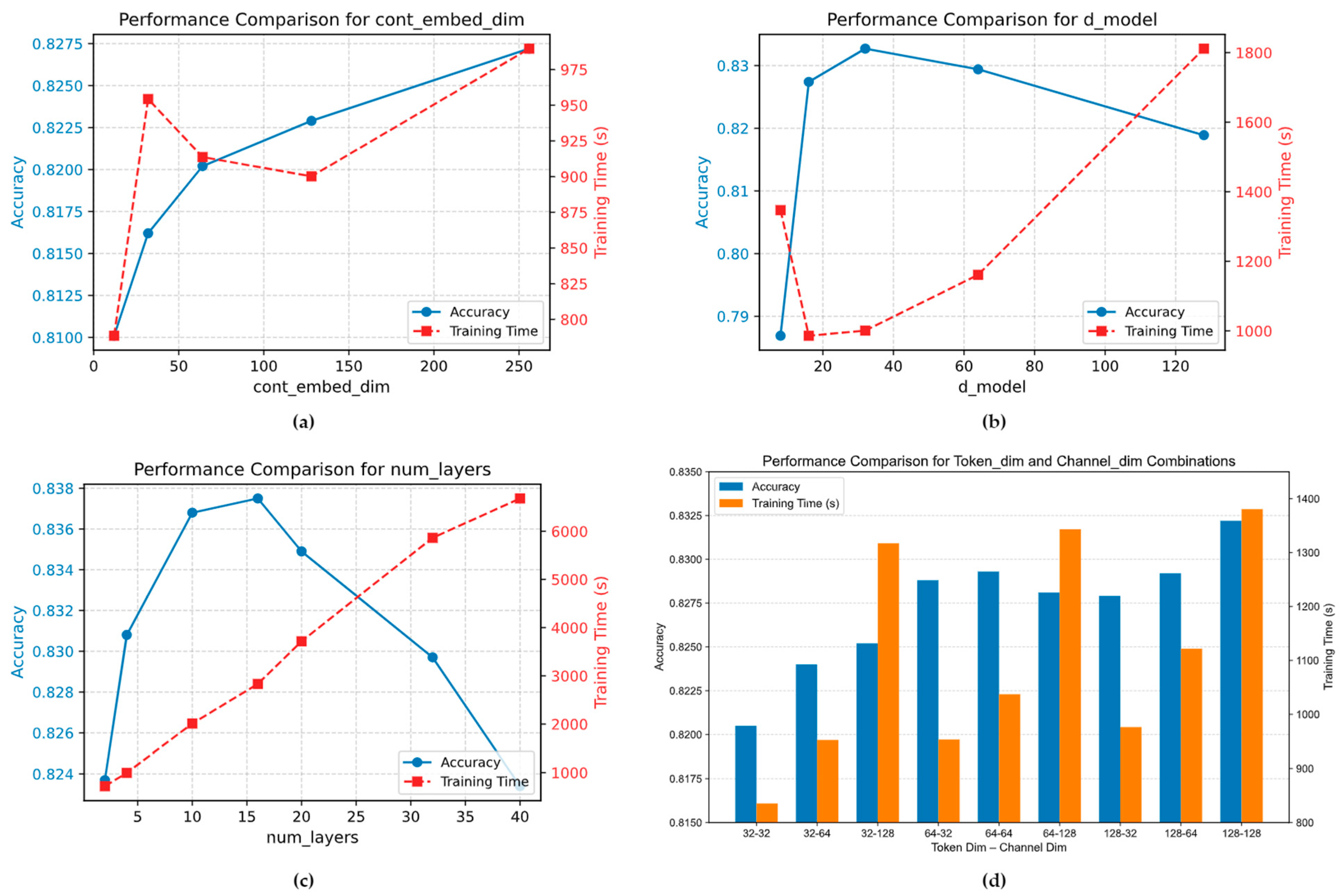
4.1. Hyperparameter Settings

This study conducted systematic tuning experiments on key hyperparameters within the network architecture. The tuning process primarily focused on four core components: the embedding dimension of continuous features (cont_embed_dim), the channel dimension of the backbone network (d_model), the number of stacked MLP-Mixer layers (num_layers), and the hidden dimensions of the Token and Channel MLPs (token_dim and channel_dim).
Each parameter was independently tested using dedicated Python scripts developed in Python 3.10. The evaluation was based on a combination of model accuracy and training time, aiming to identify optimal trade-offs between predictive performance and computational efficiency.
The results are summarized in Figure 3, which presents a comparative analysis across the four parameter categories: embedding dimensions for continuous features, backbone channel width, the number of MLP-Mixer layers, and hidden dimensions for the Token and Channel MLP components. In each subfigure, the blue curve or bar represents Accuracy (corresponding to the left Y-axis), while the orange curve or bar indicates Training Time (s) (right Y-axis), providing a visual reference for the model’s performance-efficiency tradeoff under different configurations.
Based on the overall evaluation across various performance metrics, the final model configuration was determined as follows: the embedding dimension for all continuous features (SOG, COG, relative time, longitude, and latitude) was set to 256; the backbone channel dimension (d_model) was set to 32; the number of stacked MLP-Mixer layers was set to 16; and the hidden dimensions for both the Token Mixing and Channel Mixing MLPs were set to 64.
With this configuration, the proposed model achieves a favorable balance between structural simplicity and predictive performance, providing a stable and efficient baseline for subsequent comparison experiments and ablation studies.

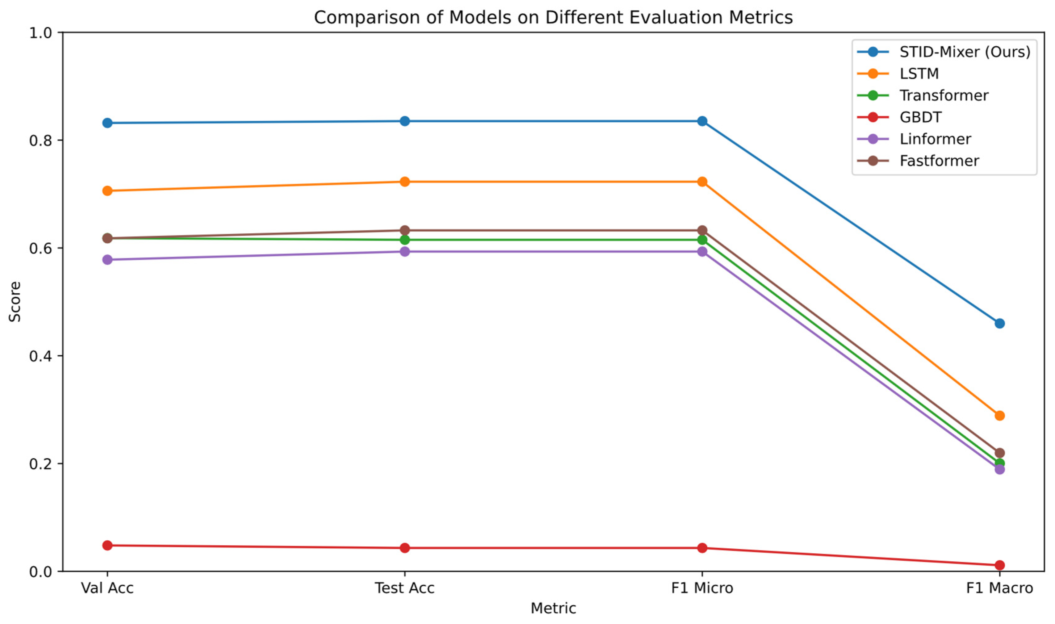
4.2. Comparative Experiments

To validate the effectiveness of the proposed STID-Mixer model in the vessel trajectory prediction task, several representative baseline methods were selected for comparison. These include traditional machine learning models (e.g., GBDT) [14], classical sequence modeling methods (e.g., LSTM and Transformer), and more recent lightweight Transformer variants (e.g., Fastformer [8] and Linformer [9]). All models were trained under a unified data preprocessing pipeline, feature construction strategy, and training configuration. Evaluation metrics include average accuracy (Accuracy), macro-averaged F1 score (F1_macro), total training time (Total Time), and average time per epoch (Time per Epoch).
As shown in Table 2 and Figure 4, the STID-Mixer model outperforms all baseline methods across all evaluation metrics. It achieves a test accuracy of 83.53%, representing improvements of approximately 11.2% and 22% over the traditional LSTM and Transformer models, respectively. Its F1_macro score reaches 0.4599, indicating that the model performs well not only on dominant classes but also demonstrates robust capability in identifying minority classes.
In contrast, GBDT (Gradient Boosted Decision Tree), as a non-sequential tree-based model, performs well in conventional classification tasks but lacks the capacity for temporal sequence modeling [31]. It fails to capture the dynamic relationships between trajectory points and cannot express the dependencies between spatial locations and temporal evolution. As a result, its performance in trajectory prediction tasks—particularly on temporally and spatially sensitive data like AIS—is significantly inferior, with both accuracy and F1 scores lagging behind deep learning-based sequence models. The LSTM (Long Short-Term Memory) model offers strong capabilities for capturing temporal dependencies and is capable of modeling trajectory dynamics to a certain extent. However, its unidirectional and sequential processing structure results in low training efficiency. Moreover, it suffers from common issues in long-sequence modeling, such as gradient vanishing or explosion. Its ability to handle high-dimensional spatiotemporal features—characteristic of AIS data—is also limited. The Transformer model, based on a self-attention mechanism, effectively captures global dependencies and offers greater modeling depth [6]. However, its computational complexity grows quadratically with sequence length, leading to substantial resource consumption and longer training times. Additionally, its modeling of temporal and spatial positions lacks structural inductive bias, making it less suited to capturing the spatial clustering and periodicity inherent in vessel behavior. Linformer and Fastformer, as lightweight Transformer variants, reduce computational overhead by introducing architectural optimizations such as linear attention and structural compression. While these models partially alleviate the computational bottlenecks of standard Transformers, they still rely on attention-based mechanisms. As a result, they struggle to adapt well to capturing localized spatial patterns and temporal regularities in AIS trajectories. Although their performance exceeds that of LSTM and standard Transformer models, they still fall short of STID-Mixer in terms of prediction accuracy and generalization ability.
The proposed STID-Mixer achieves higher accuracy and better generalization while maintaining low model complexity and computational cost. These advantages highlight its strong potential in practical trajectory prediction scenarios.

4.3. Ablation Study

To assess the contribution of each key component in the proposed STID-Mixer model, we conducted an ablation study by selectively removing different types of input features and comparing the resulting performance. Specifically, we tested the effects of retaining temporal ID features (TID), spatial ID features (SID), and a Cont-Only version that excludes all discrete identifiers and relies solely on normalized continuous AIS features. These ablated versions are compared against the full STID-Mixer architecture. Additionally, to evaluate the effectiveness of the MLP-Mixer backbone, we introduced a simplified variant named STID-MLP, which retains the complete spatiotemporal input encoding but replaces the core module with a conventional multilayer perceptron (MLP) layer.
The performance comparison across all ablated variants is summarized in Table 3. The compared models are described as follows:
  • STID-MLP: Utilizes the full set of discrete spatiotemporal features and continuous features as input but replaces the MLP-Mixer backbone with a standard multilayer perceptron.
  • SID-Mixer: Retains only the spatial discrete feature (Grid ID) while removing temporal ID features (Hour and Weekday).
  • TID-Mixer: Retains temporal ID features while removing spatial discrete input.
  • Cont-Only: A minimal version using only continuous features (SOG, COG, relative time, longitude, and latitude), with no discrete encoding.
Table 3. Comparison of ablated model performance.
Ablated ModelTest LossTest AccF1_MacroTime (s)
STID-Mixer0.72310.83530.45993452.80
STID-MLP1.60370.63660.24681000.02
SID-Mixer1.60370.63440.28434358.26
TID-Mixer3.10540.31300.07136179.84
Cont-Only3.05030.31990.06436218.47
This experiment demonstrates that the complete STID-Mixer model achieved the highest Test Accuracy and F1 Score among all ablated variants, clearly demonstrating the effectiveness and generalizability of combining spatiotemporal ID encoding (STID) with the MLP-Mixer architecture in vessel behavior modeling. In particular, the TID-Mixer variant, which retains only temporal features, suffers the most significant drop in performance, underscoring the critical role of spatial features in trajectory prediction. Notably, the Test Loss values of SID-Mixer and STID-MLP are identical at 4-decimal precision, which is a coincidence resulting from the averaging of multiple experimental runs. Despite this numerical similarity, the two models exhibit clear differences in terms of classification accuracy and macro-F1 score.
Although the STID-Mixer incurs a slightly higher runtime compared to the simpler STID-MLP model, the accuracy gains clearly validate the benefits of using MLP-Mixer for capturing temporal dependencies and feature interactions. More importantly, when compared to conventional LSTM and Transformer models, STID-Mixer delivers superior prediction accuracy with a significantly lower training cost, reflecting its lightweight and efficient design. These results confirm that all components in STID-Mixer are indispensable and jointly contribute to its strong overall performance.

5. Conclusions

This paper proposes a lightweight vessel trajectory prediction framework named STID-Mixer, which integrates Spatial-Temporal Identity (STID) encoding with a Multi-Layer Perceptron Mixer (MLP-Mixer) architecture. The model constructs a unified representation of temporal and spatial features and performs dual-axis modeling across the time and feature dimensions via the MLP-Mixer. Without relying on recurrent structures or attention mechanisms, STID-Mixer achieves strong predictive performance and high computational efficiency.
In terms of data preprocessing, a standardized pipeline was designed, including raw message parsing, trajectory segmentation, noise filtering, and feature normalization. These steps significantly enhance the usability of AIS data and contribute to the stability of model training. The input representation is composed of both discretized features—Hour, Weekday, and Grid ID—and normalized continuous variables—SOG, COG, Relative Time, Longitude, and Latitude. These inputs enable the model to effectively capture trajectory patterns. The MLP-Mixer serves as the core modeling backbone, allowing efficient parallel computation while learning temporal dependencies and feature interactions.
Extensive experiments on real-world AIS datasets show that STID-Mixer achieves a Top-1 accuracy of 84.34%, outperforming classical baselines such as LSTM, Transformer, and GBDT by a significant margin. Moreover, the model demonstrates lower training costs compared to deep recurrent or attention-based models, confirming its scalability and deployment potential. Ablation studies further verify that both the STID module and the MLP-Mixer structure contribute significantly to the model’s performance.
Despite its promising results, this work has several limitations. The current model does not explicitly account for inter-vessel interactions, which may be crucial in dense traffic environments. Future work could explore graph-based architectures, such as Graph Neural Networks (GNNs), to model cooperative dynamics among multiple vessels. Moreover, multi-step trajectory forecasting and the modeling of behavioral uncertainty remain open challenges worth further investigation.
In conclusion, STID-Mixer offers a compact, efficient, and accurate framework for AIS trajectory modeling. Its flexibility and effectiveness make it well-suited for a range of maritime applications, including intelligent navigation, route planning, and anomaly detection. This study also lays a foundation for future research into scalable, data-driven maritime behavior prediction systems.

Author Contributions

Conceptualization, L.W. and G.J.; methodology, G.J.; software, L.W.; validation, L.W.; formal analysis, L.W.; investigation, X.D.; data curation, X.D.; writing—original draft preparation, L.W.; writing—review and editing, J.Z.; visualization, L.W.; supervision, J.Z. All authors have read and agreed to the published version of the manuscript.

Funding

This research received no external funding.

Institutional Review Board Statement

Not applicable.

Informed Consent Statement

Not applicable.

Data Availability Statement

Restrictions apply to the availability of these data. Data were obtained from the South China Sea Navigation Service Center of the China Maritime Safety Administration and are available at https://enav.nhhb.org.cn/nbwebgis/(accessed on 15 June 2024) with the permission of the China Maritime Safety Administration. Interested researchers may contact the authors to obtain detailed information on the temporal and geographical scope of the dataset before applying for access from the official source.

Acknowledgments

The authors would like to thank their supervisor for his guidance and to the other authors for their assistance in this manuscript.

Conflicts of Interest

The authors declare no conflicts of interest.

Abbreviations

The following abbreviations are used in this manuscript:
AISAutomatic Identification System
MMSIMaritime Mobile Service Identity
LONLongitude
LATLatitude
SOGSpeed Over Ground
COGCourse Over Ground
VHFVery High Frequency
STIDSpatial-Temporal Identity
MLPMultilayer Perceptron
RNNRecurrent Neural Network
LSTMLong Short-Term Memory
TREADTrajectory Reconstruction and Evaluation for Anomaly Detection
SGCNSparse Graph Convolutional Network
MTSMultivariate Time Series
GBDTGradient Boosted Decision Tree
GELUGaussian Error Linear Unit

References

  1. Murray, B.; Perera, L.P. An AIS-based deep learning framework for regional ship behavior prediction. Reliab. Eng. Syst. Saf. 2021, 215, 107819. [Google Scholar] [CrossRef]
  2. Hexeberg, S.; Flåten, A.L.; Brekke, E.F. AIS-based vessel trajectory prediction. In Proceedings of the 2017 20th international conference on information fusion (Fusion), Xi’an, China, 10–13 July 2017; pp. 1–8. [Google Scholar]
  3. Yang, D.; Wu, L.; Wang, S.; Jia, H.; Li, K.X. How big data enriches maritime research–a critical review of Automatic Identification System (AIS) data applications. Transp. Rev. 2019, 39, 755–773. [Google Scholar] [CrossRef]
  4. Mazzarella, F.; Arguedas, V.F.; Vespe, M. Knowledge-based vessel position prediction using historical AIS data. In Proceedings of the 2015 Sensor Data Fusion: Trends, Solutions, Applications (SDF), Bonn, Germany, 6–8 October 2015; pp. 1–6. [Google Scholar]
  5. Rong, H.; Teixeira, A.; Soares, C.G. Ship trajectory uncertainty prediction based on a Gaussian Process model. Ocean Eng. 2019, 182, 499–511. [Google Scholar] [CrossRef]
  6. Vaswani, A.; Shazeer, N.; Parmar, N.; Uszkoreit, J.; Jones, L.; Gomez, A.N.; Kaiser, Ł.; Polosukhin, I. Attention is all you need. In Proceedings of the Advances in Neural Information Processing Systems 30 (NeurIPS 2017), Long Beach, CA, USA, 4–9 December 2017. [Google Scholar]
  7. Wu, H.; Xu, J.; Wang, J.; Long, M. Autoformer: Decomposition transformers with auto-correlation for long-term series forecasting. In Proceedings of the Advances in Neural Information Processing Systems 34 (NeurIPS 2021), Virtual, 6–14 December 2021; pp. 22419–22430. [Google Scholar]
  8. Wu, C.; Wu, F.; Qi, T.; Huang, Y.; Xie, X. Fastformer: Additive attention can be all you need. arXiv 2021, arXiv:2108.09084. [Google Scholar]
  9. Wang, S.; Li, B.Z.; Khabsa, M.; Fang, H.; Ma, H. Linformer: Self-attention with linear complexity. arXiv 2020, arXiv:2006.04768. [Google Scholar]
  10. Zhou, H.; Zhang, S.; Peng, J.; Zhang, S.; Li, J.; Xiong, H.; Zhang, W. Informer: Beyond efficient transformer for long sequence time-series forecasting. In Proceedings of the AAAI conference on artificial intelligence, Virtual, 2–9 February 2021; pp. 11106–11115. [Google Scholar]
  11. Pallotta, G.; Vespe, M.; Bryan, K. Vessel pattern knowledge discovery from AIS data: A framework for anomaly detection and route prediction. Entropy 2013, 15, 2218–2245. [Google Scholar] [CrossRef]
  12. Li, S.; Jin, X.; Xuan, Y.; Zhou, X.; Chen, W.; Wang, Y.-X.; Yan, X. Enhancing the locality and breaking the memory bottleneck of transformer on time series forecasting. In Proceedings of the Advances in Neural Information Processing Systems 32 (NeurIPS 2019), Vancouver, BC, Canada, 8–14 December 2019. [Google Scholar]
  13. Li, H.; Jiao, H.; Yang, Z. AIS data-driven ship trajectory prediction modelling and analysis based on machine learning and deep learning methods. Transp. Res. E Logist. Transp. Rev. 2023, 175, 103152. [Google Scholar] [CrossRef]
  14. Friedman, J.H. Greedy function approximation: A gradient boosting machine. Ann. Stat. 2001, 29, 1189–1232. [Google Scholar] [CrossRef]
  15. Xiao, F.; Ligteringen, H.; Van Gulijk, C.; Ale, B. Comparison study on AIS data of ship traffic behavior. Ocean Eng. 2015, 95, 84–93. [Google Scholar] [CrossRef]
  16. Tu, E.; Zhang, G.; Rachmawati, L.; Rajabally, E.; Huang, G.-B. Exploiting AIS data for intelligent maritime navigation: A comprehensive survey from data to methodology. IEEE Trans. Intell. Transp. Syst. 2017, 19, 1559–1582. [Google Scholar] [CrossRef]
  17. Ristic, B.; La Scala, B.; Morelande, M.; Gordon, N. Statistical analysis of motion patterns in AIS data: Anomaly detection and motion prediction. In Proceedings of the 2008 11th International Conference on Information Fusion, Cologne, Germany, 30 June–3 July 2008; pp. 1–7. [Google Scholar]
  18. Gao, M.; Shi, G.; Li, S. Online prediction of ship behavior with automatic identification system sensor data using bidirectional long short-term memory recurrent neural network. Sensors 2018, 18, 4211. [Google Scholar] [CrossRef] [PubMed]
  19. Schmidt, R.M. Recurrent neural networks (rnns): A gentle introduction and overview. arXiv 2019, arXiv:1912.05911. [Google Scholar]
  20. Fang, W.; Chen, Y.; Xue, Q. Survey on research of RNN-based spatio-temporal sequence prediction algorithms. J. Big Data 2021, 3, 97. [Google Scholar] [CrossRef]
  21. Forti, N.; Millefiori, L.M.; Braca, P.; Willett, P. Prediction oof vessel trajectories from AIS data via sequence-to-sequence recurrent neural networks. In Proceedings of the ICASSP 2020-2020 IEEE International Conference on Acoustics, Speech and Signal Processing (ICASSP), Virtual, 4–8 May 2020; pp. 8936–8940. [Google Scholar]
  22. Shi, L.; Wang, L.; Long, C.; Zhou, S.; Zhou, M.; Niu, Z.; Hua, G. SGCN: Sparse graph convolution network for pedestrian trajectory prediction. In Proceedings of the 2021 IEEE/CVF Conference on Computer Vision and Pattern Recognition (CVPR), Virtual, 20–25 June 2021; pp. 8994–9003. [Google Scholar]
  23. Cheng, J.C.; Poon, K.H.; Wong, P.K.-Y. Long-Time gap crowd prediction with a Two-Stage optimized spatiotemporal Hybrid-GCGRU. Adv. Eng. Inform. 2022, 54, 101727. [Google Scholar] [CrossRef]
  24. Lin, Z.; Yue, W.; Huang, J.; Wan, J. Ship trajectory prediction based on the TTCN-attention-GRU model. Electronics 2023, 12, 2556. [Google Scholar] [CrossRef]
  25. Shao, Z.; Zhang, Z.; Wang, F.; Wei, W.; Xu, Y. Spatial-temporal identity: A simple yet effective baseline for multivariate time series forecasting. In Proceedings of the 31st ACM International Conference on Information and Knowledge Management(CIKM 2022), Atlanta, GA, USA, 17–21 October 2022; pp. 4454–4458. [Google Scholar]
  26. Tolstikhin, I.O.; Houlsby, N.; Kolesnikov, A.; Beyer, L.; Zhai, X.; Unterthiner, T.; Yung, J.; Steiner, A.; Keysers, D.; Uszkoreit, J. Mlp-mixer: An all-mlp architecture for vision. In Proceedings of the Advances in Neural Information Processing Systems 34 (NeurIPS 2021), Virtual, 6–14 December 2021; pp. 24261–24272. [Google Scholar]
  27. Ekambaram, V.; Jati, A.; Nguyen, N.; Sinthong, P.; Kalagnanam, J. Tsmixer: Lightweight mlp-mixer model for multivariate time series forecasting. In Proceedings of the 29th ACM SIGKDD Conference on Knowledge Discovery and Data Mining (KDD ‘23), Long Beach, CA, USA, 6–10 August 2023; pp. 459–469. [Google Scholar]
  28. Chen, S.-A.; Li, C.-L.; Yoder, N.; Arik, S.O.; Pfister, T. Tsmixer: An all-mlp architecture for time series forecasting. arXiv 2023, arXiv:2303.06053. [Google Scholar]
  29. National Marine Electronics Association. NMEA 0183 Standard for Interfacing Marine Electronic Devices. Available online: https://www.nmea.org/nmea-0183.html (accessed on 10 June 2024).
  30. China MSA AIS Service Platform. Available online: https://enav.nhhb.org.cn/nbwebgis/ (accessed on 15 June 2024).
  31. Li, Q.; Wang, Y.; Shao, Y.; Li, L.; Hao, H. A comparative study on the most effective machine learning model for blast loading prediction: From GBDT to Transformer. Eng. Struct. 2023, 276, 115310. [Google Scholar] [CrossRef]
Figure 1. STID-Mixer consists of STID Layer, Mixer layers, and a classifier head. STID Layer contains one encoding layer and one embedding layer. Mixer layers contain one token-mixing MLP and one channel-mixing MLP, each consisting of two fully connected layers and a GELU nonlinearity. Other components include skip-connections, dropout, and layer norm on the channels.
Eng 06 00184 g001
Figure 2. A trajectory segment visualized within a sample 5 × 5 spatial grid region.
Eng 06 00184 g002
Figure 3. Comparative results for hyperparameter tuning: (a) Effect of the embedding dimension for continuous features (cont_embed_dim); (b) Effect of the backbone channel dimension (d_model); (c) Effect of the number of stacked Mixer layers (num_layers); (d) Combined effect of hidden dimensions in Token and Channel MLPs (token_dim–channel_dim). In each subfigure, blue represents accuracy and orange denotes training time (s).
Eng 06 00184 g003
Figure 4. Comparison of different models on validation accuracy, test accuracy, F1-micro, and F1-macro metrics.
Eng 06 00184 g004
Table 1. An example of structured AIS trajectory samples after spatio-temporal encoding and preprocessing. The selected features include static identifiers (MMSI, traj_id), temporal attributes (hour, weekday, relative time), spatial coordinates (LON, LAT, Grid_id), and navigational dynamics (SOG, COG).
MMSITimeHourWeekdayLONLATGrid_idSOGCOGTraj_id
1008990430.58501110.93830.0032470.05670.9250100899043_2
1008990430.58501110.93740.0050470.05570.9269100899043_2
1008990430.58511110.93480.0121470.05380.9272100899043_2
Table 2. Comparison of different models on the AIS trajectory prediction task.
ModelsVal AccTest AccF1_MacroTotal Time (s)Time/Epoch (s)
STID-Mixer0.83190.83530.45993452.80215.80
LSTM0.70600.72290.288819,342.97452.76
Transformer0.61820.61510.200317,449.81667.90
GBDT0.04810.04340.011323,937.32 
Linformer0.57820.59330.18916255.08235.23
Fastformer0.61790.63260.219614,318.40505.40
Disclaimer/Publisher’s Note: The statements, opinions and data contained in all publications are solely those of the individual author(s) and contributor(s) and not of MDPI and/or the editor(s). MDPI and/or the editor(s) disclaim responsibility for any injury to people or property resulting from any ideas, methods, instructions or products referred to in the content.

