Cauchy Operator Boosted Artificial Rabbits Optimization for Solving Power System Problems

Abstract

The majority of the challenges faced in power system engineering are presented as constrained optimization functions, which are frequently characterized by their complicated architectures. Metaheuristics are mathematical techniques used to solve complicated optimization problems. One such technique, Artificial Rabbits Optimization (ARO), has been designed to address global optimization challenges. However, ARO has limitations in terms of search functionality, restricting its efficiency in dealing with constrained optimization environments. To improve ARO’s compatibility with a variety of challenging problems, this work proposes implementing the Cauchy mutation operator into the position-updating procedure during the exploration stage. Furthermore, a novel multi-mode control parameter is developed to facilitate a smooth transition between exploration and exploitation phases. The enhancements may boost the performance and serve as an effective optimization tool for tackling complex engineering tasks. The improved version is known as Cauchy Artificial Rabbits Optimization (CARO). The proposed CARO’s performance is evaluated using eleven power system challenges as part of the CEC2020 competition’s test set of real-world constrained problems. The experimental results demonstrate the practical applicability of the proposed CARO in engineering applications and provide areas for future investigation.

1. Introduction

Enhancing power system efficiency corresponds with the objectives of sustainable development. The increasing implementation of renewable energy sources and the substantial integration of contemporary ICT technologies have led to significant transformations in power systems [1]. Demand response programs, which incentivize users to modify their consumption behaviors at peak periods when electricity is costly or sourced from non-renewable resources, are facilitated by the integration of smart grid technologies into power systems. These programs assist consumers in utilizing power more effectively and promote environmental sustainability [2]. Nonetheless, such advances could lead to increased difficulties in system management and operation. Effective optimization approaches are necessary to tackle various power optimization challenges.

Metaheuristic algorithms have garnered significant interest over the past decades and have become a prevalent method for tackling complex real-world optimization challenges [3]. Their principal benefit over conventional mathematical programming methods is in their capacity to solve optimization problems by exclusively evaluating fitness functions and their constraints without the need for gradient information. Additionally, the search agents in these algorithms display stochastic tendencies that give them the ability to do global searches [4].

Optimization problems that arise from practical applications and exhibit high complexity are referred to as real-world problems. It’s worth noting that non-convex and non-linear constraints are common in real-world optimization challenges [5]. The constrained nature of these problems, coupled with the relatively smaller feasible regions within the decision variable space, can potentially diminish the efficiency of any optimizer. Furthermore, it’s worth mentioning that most of the optimization methods are primarily intended to deal with unconstrained optimization problems. Consequently, constraints should be handled using appropriate techniques to address the equality and inequality restrictions inherent in real-world problems [6].

Metaheuristics are problem-solving techniques that replicate various natural phenomena, including biological processes, physical laws, and chemical reactions. These algorithms are generally categorized into four primary groups depending on their source of inspiration: (1) Evolutionary-based algorithms, (2) Swarm intelligence-based algorithms, (3) Natural science-based algorithms (4) Human-based algorithms [7]. Evolutionary-based methodologies are rooted in the principles of natural evolution. These methods typically initiate the search process by generating an initial population through randomization, thereafter exposing this population to a multi-generational evolutionary advancement. The scientific literature provides numerous examples of procedures classified as evolutionary-based. Notably, Genetic Algorithm (GA) [8] stands out as one of the most renowned algorithms in this category and draws its inspiration from Darwin’s theory of evolution. Furthermore, this category encompasses other techniques like Differential Evolution (DE) [9].

The second category of methodologies comprises swarm intelligence-based algorithms. This category of metaheuristics is highly regarded, as it mimics the cooperative, adaptive, cognitive, and collective social behaviors found in natural communities and groupings. These natural assemblages include a diverse range of organisms, such as schools of fish, flocks of birds, herds of mammals, colonies of insects like bees, and several other species. The domain of swarm intelligence algorithms is extensive and varied. Among them, the most renowned is Particle Swarm Optimization (PSO) [10], which models the flocking behavior of birds. There are also other notable algorithms in this category, including but not limited to the Nutcracker Optimizer (NO) [11], Giant Trevally Optimizer (GTO) [12], and Draco Lizard Optimizer (DLO) [13].

Alternatively, algorithms grounded in natural science replicate particular physical phenomena or chemical principles, such as electrical charges, gravity, and ion movement, among others. The Black Hole Algorithm (BHA) [14] is a prominent algorithm in this domain, drawing inspiration from the behavior of black holes in astrophysics, namely their ability to attract and assimilate matter. Some other notable methods falling into this group include Archimedes Optimization Algorithm (AOA) [15], Energy Valley Optimizer (EVO) [16], and several others.

The last classification of these algorithms belongs to human-based methods. These methods take inspiration from human cooperation and community behavior. Some of the most widely recognized algorithms within this category include the Brain Storm Optimization (BSO) [17], Group Teaching Optimization Algorithm (GTOA) [18], among others.

Given their ability to offer precise and flexible optimization solutions for various complex real-world problems, metaheuristic algorithms have been extensively employed in tackling engineering optimization challenges in various domains. These applications encompass a diverse spectrum of fields, including applied mechanics and engineering [19,20], parameter estimation of photovoltaic models [21,22], maximum power point tracking of generation systems [23,24], classification problems [25,26], power system stabilizer [27], image segmentation [28], constrained engineering optimization [29,30], feature selection [31,32], global optimization [33,34], machine learning model optimization [35], optimum design of truss structures [36], optimize the deployment of distribution-static VAR compensator [37], internet of things systems [38], intrusion detection system [39], optimal placement of unified power flow controller [40], vehicle routing [41], large-scale optimization [42].

Metaheuristic algorithms are typically structured around two fundamental phases: exploration (diversification) and exploitation (intensification). Achieving an optimal equilibrium between these phases is imperative for the efficiency and robustness of metaheuristic algorithms, thereby ensuring superior outcomes within specific applications [7]. The exploration phase is centered on the exploration of remote regions within the solution space to detect improved candidate solutions. Following the exploration phase, a thorough examination of the search space is essential. The method navigates feasible areas of the search space and seeks to identify the optimal solution through several local convergence strategies [43].

Studies have demonstrated the exceptional ability of specific metaheuristic algorithms to rapidly achieve high-quality solutions, efficiently solving complicated issues. These advanced algorithms aim to enhance aims and effectively determine ideal solutions through the use of search agents. During exploration, it is crucial that candidate solutions demonstrate a high success rate in identifying the ideal selection [44]. Notably, some of these candidates may prematurely converge to local optima, inaccurately assuming them to be the global optimum. Consequently, there is an imperative need for a comprehensive exploration of candidate solutions within the solution space to ensure the discovery of the true global optimum. The vital prerequisites for metaheuristic algorithms to effectively address engineering optimization problems encompass striking the right balance between diversification and intensification, as well as guarding against the entrapment in local optima. This equilibrium serves to facilitate a comprehensive exploration of the solution space and, in parallel, ensures the successful acquisition of the optimal global solution [45].

The Artificial Rabbits Optimization (ARO), presented by Wang et al. [46], is a recent development in the field. ARO draws influence from the survival tactics of wild rabbits, including their methods of detour foraging and random concealment. In ARO, detour foraging represents the exploration phase, whereas random hiding signifies the exploitation phase. Although ARO demonstrates strong exploitation skills, it struggles with an inconsistent exploration phase, which sometimes results in convergence to local optima, particularly in complicated and high-dimensional challenges [47].

In this study, ARO was selected as the base algorithm due to its promising characteristics in balancing exploration and exploitation phases through detour foraging and random hiding strategies. Its simplicity and flexibility make it a suitable candidate for adaptation to complex, constrained optimization problems such as power system challenges. Moreover, recent empirical studies [46] have demonstrated its competitive performance in engineering applications. However, ARO’s limitations in handling exploration under strict constraints motivated the incorporation of the Cauchy mutation operator in this work, aiming to further enhance its performance for power system problems.

The motivation behind this design choice is based on both theoretical foundations and empirical evidence from prior metaheuristic research. Specifically:

(1)

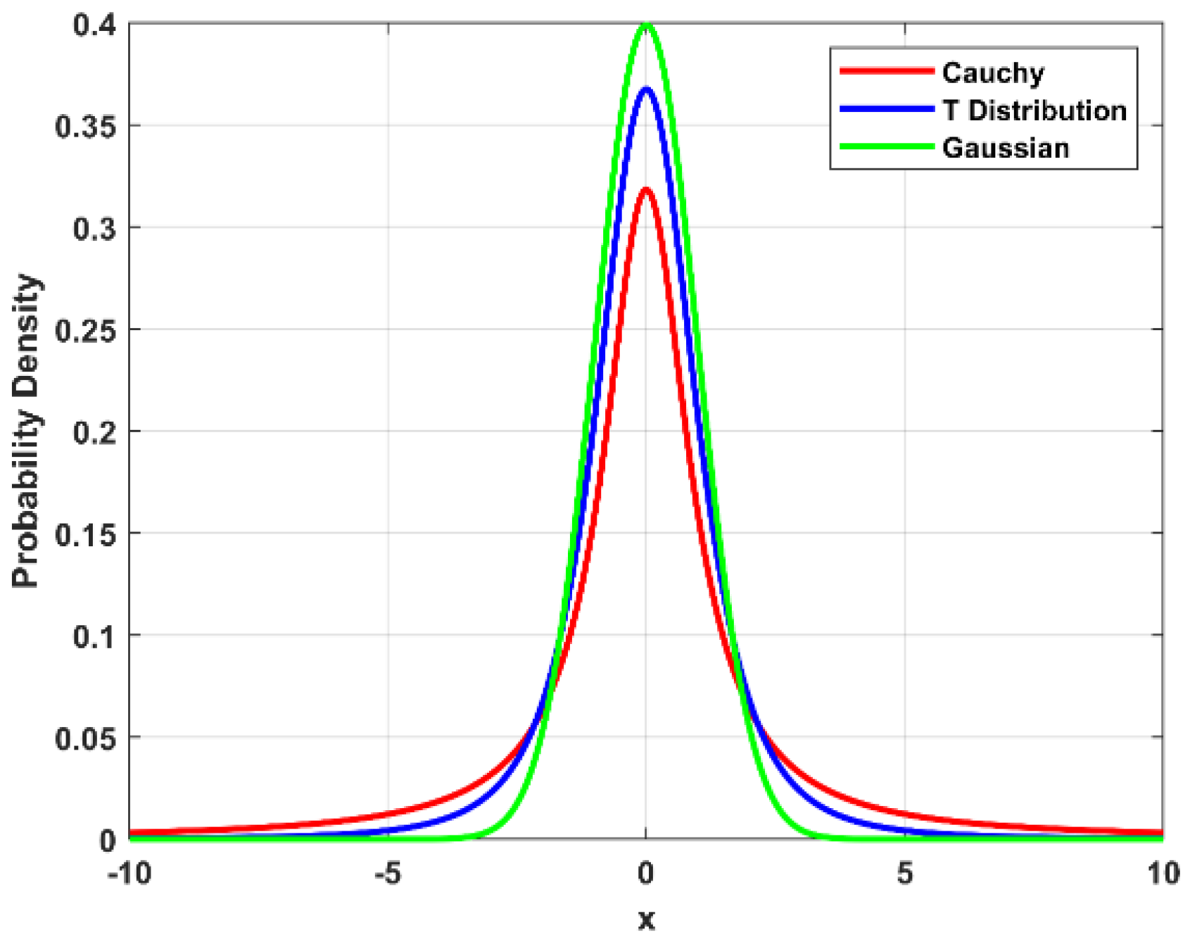
Heavy-Tailed Distribution Advantage: The Cauchy distribution is characterized by its heavy tails and undefined mean and variance. This property allows the mutation to produce occasional large jumps in the search space, which enhances global exploration and mitigates the risk of premature convergence to local optima, which is a common limitation observed in standard ARO, especially in constrained high-dimensional problems.

(2)

Enhanced Exploration Capability: By introducing the Cauchy mutation in the exploration phase, the algorithm gains an increased ability to escape local optima and conduct broader searches across the solution space, leading to a more thorough investigation of potential optimal regions.

(3)

Convergence Acceleration: While promoting exploration, the probabilistic nature of the Cauchy operator also permits fine-tuning around promising areas due to the frequent occurrence of smaller steps near the distribution center, thus supporting a more balanced transition between exploration and exploitation.

(4)

Supporting Empirical Studies: Prior studies, such as the work on Cauchy mutation-enhanced Harris Hawks Optimization [48], have empirically demonstrated the effectiveness of this approach in improving both convergence speed and solution accuracy in various engineering optimization problems. This empirical background provided a solid basis for adopting a similar strategy in enhancing ARO.

Motivated by the advantages of the Cauchy mutation operator and recognizing the limitations of ARO, a novel algorithm called Cauchy Artificial Rabbits Optimization (CARO) is proposed in this study. Eleven challenging power system problems from CEC2020 constrained benchmark functions have been used to seek the applicability of CARO while solving real-world problems. To evaluate the CARO performance, the results of the experiments were compared to various well-known recently developed algorithms.

The key contributions of the paper can be summarized as follows:

(1)

A novel optimization framework has been proposed by enhancing the Artificial Rabbits Optimization (ARO) algorithm with a Cauchy mutation operator and a multi-mode energy shrink control parameter, providing an effective structure for solving complex constrained engineering problems.

(2)

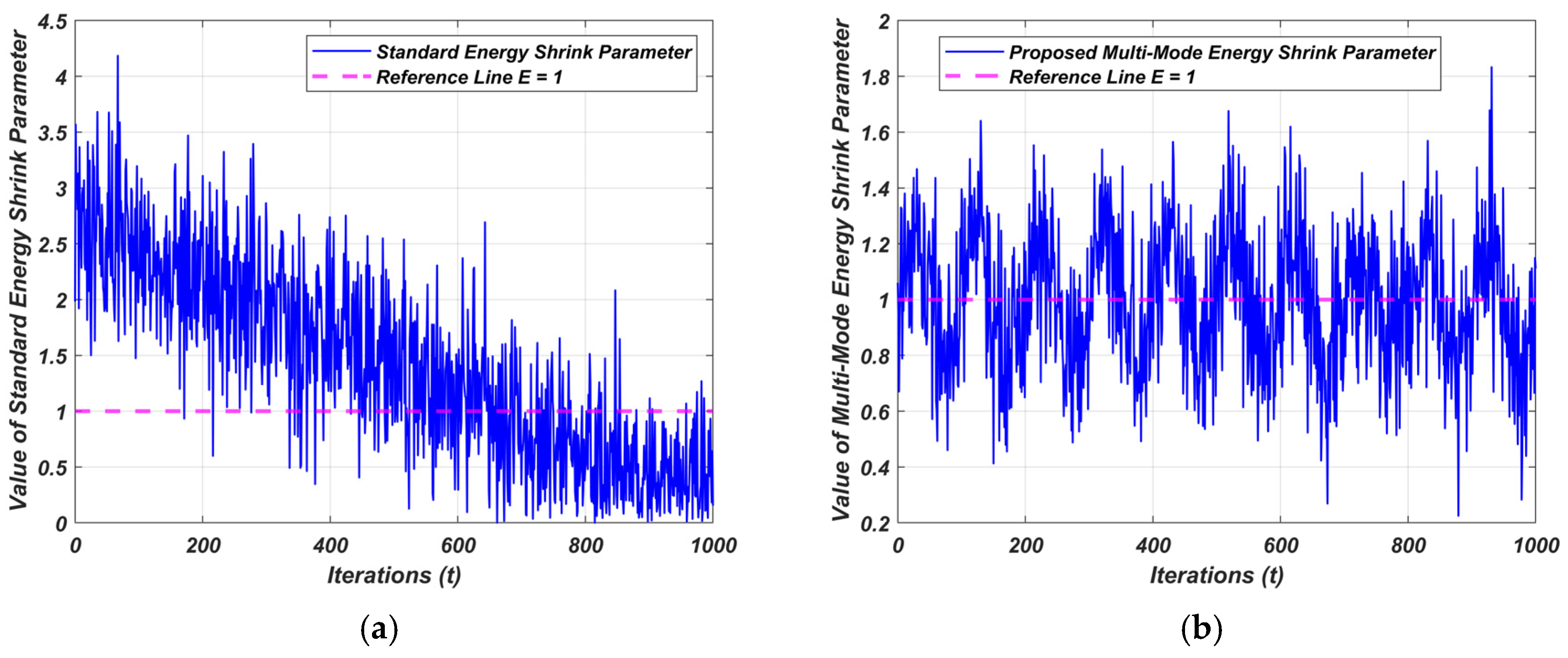
The main improvement in comparison to the standard ARO focuses on enhancing the exploration phase and reducing the probability of becoming trapped in local optima. This enhancement is achieved by introducing the Cauchy mutation operator. Additionally, proposing a novel multi-mode control parameter that allows for a seamless transition between exploration and exploitation, avoiding premature convergence and ultimately increasing the exploration and exploitation potential of the search space.

(3)

The proposed CARO is applied to eleven power system problems derived from IEEE CEC2020 constrained engineering benchmark functions. The superiority of CARO has been noticed using different metrics. Comprehensive evaluation criteria are used. These criteria are: best, mean, worst, std, and spider plots.

The remainder of this paper is organized as follows. Section 2 explains the Artificial Rabbits Optimization (ARO). Section 3 describes the Proposed CARO. Section 4 is about power system problems. Performance evaluation and discussion of results when the CARO algorithm is applied over power system challenges are presented in Section 5. The conclusions and future works are presented in Section 6.

2. Artificial Rabbits Optimization (ARO)

This algorithm is inspired by the survival strategies observed in rabbits within their natural habitat. These strategies encompass the detour foraging approach, where rabbits explore the surroundings of their nests in search of sustenance. In addition, rabbits employ a random hiding strategy, constructing burrows around their nests and intermittently seeking shelter within them to evade potential threats from hunters and predators. These tactical transitions are influenced by fluctuations in their energy levels [46].

2.1. Detour Foraging (Exploration)

In this step, each rabbit in the swarm typically updates its position by shifting towards a randomly chosen member of the group, while also introducing a perturbation. The mathematical representation of the detour foraging process is given by the following equation:

$$Rab{b}_{new}={\overrightarrow{x}}_j+R\times \left({\overrightarrow{x}}_i-{\overrightarrow{x}}_j\right)+round\left(0.5\times \left(0.05+r_1\right)\right)\times n_1,i,j=1,\dots ,and i\ne j$$

(1)

$$R=L\times m$$

(2)

$$L=\sin \left(2\pi r_2\right)\times \left(e-e^{{\left({\displaystyle \frac{t-1}{T}}\right)}^2}\right)$$

(3)

$$\begin{array}{c}m\left(k\right)=\left\{\begin{array}{l}0\\ 1\end{array}\right.\hspace{1em}if k==g\left(l\right)\\ else\\ k=1,\dots ,d and l=1,\dots ,\left[r_3\cdot d\right]\end{array}$$

(4)

$$g=randperm\left(d\right)$$

(5)

$$n_1~N\left(0,1\right)$$

(6)

where ${Rabb}_{new}$ represents the potential location of the ith rabbit in the subsequent iteration, denoted as t + 1. ${\overrightarrow{X}}_i$ and ${\overrightarrow{X}}_j$ signify the current positions of the ith and jth rabbits, respectively, during iteration t. n corresponds to the population size. t is the current iteration count. T is the maximum allowable number of iterations. d represents the dimensionality of the specific problem. The notation [·] indicates the ceiling function, while $round$ (·) signifies rounding to the nearest $randperm$ (·) refers to the selection of a random integer within the range of 1 to d. $r_1, r_2, and r_3$ are all random numbers falling within [0, 1]. $n_1$ represents the normal distribution. $L$ denotes the distance covered in each step of the exploration stage.

2.2. Random Hiding (Exploitation)

In the context of evading predators, rabbits typically dig burrows near their nests for concealment. The equation related to this behavior is as follows:

$${\overrightarrow{b}}_{i,j}={\overrightarrow{X}}_i+H\times g\times {\overrightarrow{X}}_{i,j}=1,\dots \begin{array}{ccc}n& \mathrm{a}\mathrm{n}\mathrm{d}& j\end{array}=1,\dots ,d$$

(7)

$$H={\displaystyle \frac{T-t+1}{T}}\times r_4$$

(8)

$$n_2~N\left(0,1\right)$$

(9)

$$g\left(k\right)=\left\{\begin{array}{c}1\\ 0\end{array}\begin{array}{cc}if& k==j\\ else& k=1,\dots ,d\end{array}\right.$$

(10)

In their quest for survival, rabbits must find secure shelter to evade threats. Consequently, they randomly choose one of their burrows to hide in and avoid capture. This representation of the random hiding strategy is expressed below:

$$Rab{b}_{new}={\overrightarrow{X}}_i+R\times \left(r_4\times \left({\overrightarrow{b}}_{ir}-{\overrightarrow{X}}_i\right)\right),i=1,\dots ,n$$

(11)

$$g_r\left(k\right)=\left\{\begin{array}{c}1\\ 0\end{array}\begin{array}{cc}if& k==\left[r_5\cdot d\right]\\ else& k=1,\dots ,d\end{array}\right.$$

(12)

$${\overrightarrow{b}}_{i,r}={\overrightarrow{X}}_i+H\times g_r\times {\overrightarrow{X}}_i$$

(13)

Here, ${\overrightarrow{b}}_{i,r}$ denotes the randomly chosen burrow of the ith rabbit from a set of d burrows used for hiding in the current iteration t. Additionally, $r_4$ and $r_5$ are two random numbers generated from the interval [0, 1], and $n_2$ represents the normal distribution.

Following either the first or the second step of the algorithm, the position of the ith rabbit is updated as follows:

$${\overrightarrow{X}}_i\left(t+1\right)=\left\{\begin{array}{c}{\stackrel{\rightharpoonup }{X}}_i\\ Rab{b}_{new}\end{array}\begin{array}{cc}if& f\left({\stackrel{\rightharpoonup }{X}}_i\le Rab{b}_{new}\right)\\ if& f\left({\stackrel{\rightharpoonup }{X}}_i>Rab{b}_{new}\right)\end{array}\right.$$

(14)

According to the above equation, the rabbit will forsake its current location and choose to remain at the candidate position generated by either Equation (1) or Equation (11) if the fitness of the ith rabbit’s candidate position is greater than the fitness of the present position.

2.3. Energy Shrink (Switch from Exploration to Exploitation)

An energy factor is employed to signify the transition from the exploration phase to the exploitation phase and can be expressed in the following manner:

$$A\left(t\right)=4\left(1-{\displaystyle \frac{t}{T}}\right)\ln {\displaystyle \frac{1}{r}}$$

(15)

where $r$ randomly generated from [0, 1]. The energy coefficient $A$ takes values within the interval [0, 2]. If $A$ > 1, it signifies that the rabbit possesses ample energy for extensive exploration of the foraging area of various individuals, leading to the detour foraging phase. This phase is characterized as exploration. Conversely, when $A$ ≤ 1, it indicates that the rabbit has limited energy for physical activities. Consequently, it resorts to random hiding as a means of evading predators, and this marks the exploitation phase in the algorithm.

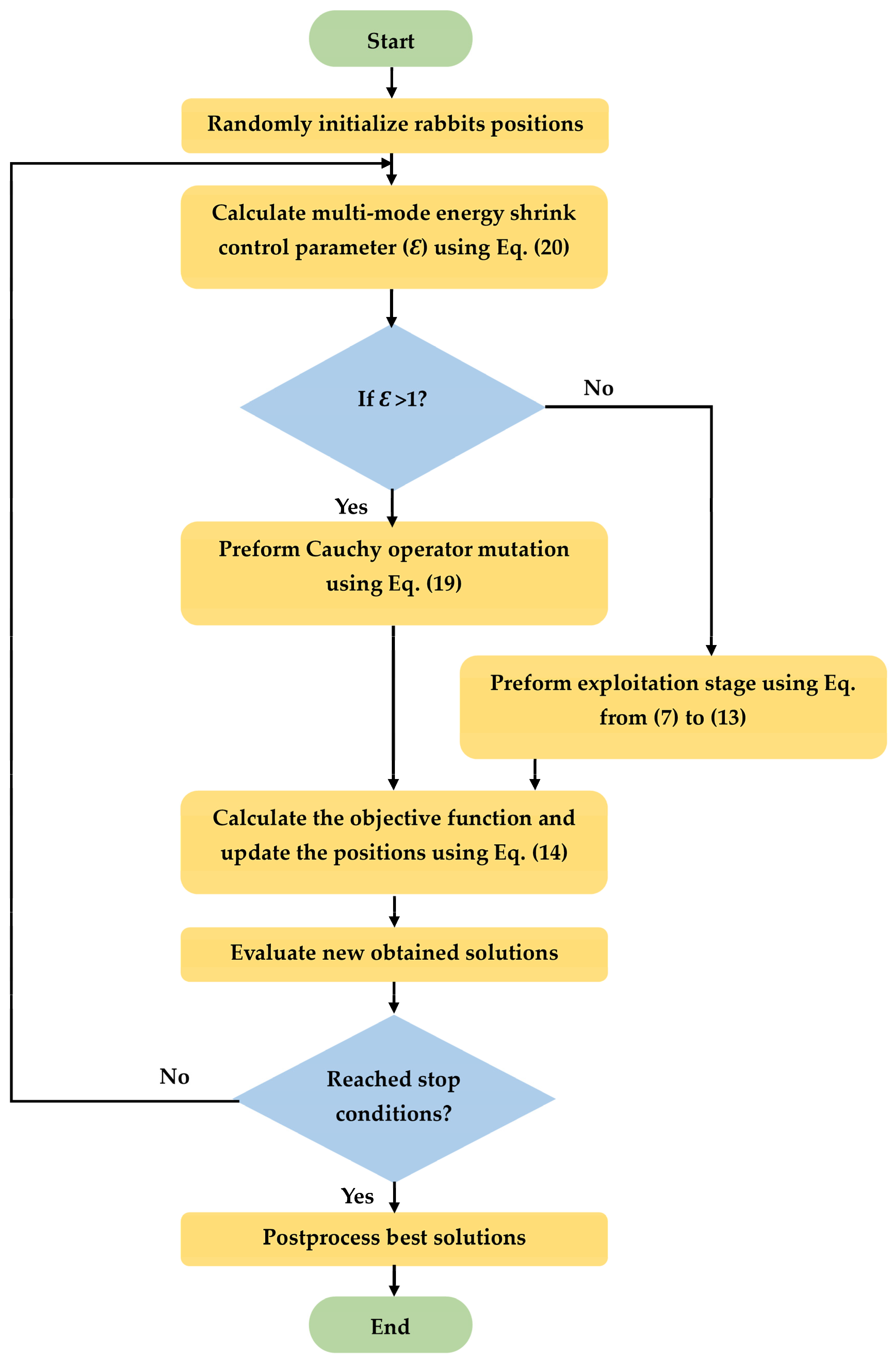
3. Proposed Cauchy Artificial Rabbits Optimization (CARO)

The optimal direction in the swarm is guided by the best agent, making a proper balance between diversification and intensification vital for search algorithms. These factors are key in the search for problem optima. Typically, in each iteration, the standard ARO employs a detour foraging strategy to move closer to the optima, facilitating the solution of complex real-world problems. However, there are instances where this movement is insufficient to prevent the swarm from becoming trapped in local optima. To address this issue, this paper proposes an enhanced version of the original ARO algorithm by incorporating a Cauchy mutation operator. The algorithm incorporates the Cauchy operator to facilitate exploration of the search space by moving towards the best solution. The Cauchy operator employed here utilizes Cauchy random numbers. These numbers have the potential to trigger significant jumps from the current best agent, facilitating sudden transitions from local optima to exploring the entire search space.

This mechanism aims to expedite convergence and prevent premature convergence. The use of Cauchy-distributed random numbers has been proven effective in producing high-quality solutions [48].

3.1. Cauchy Distribution

The Cauchy distribution is a probability distribution used in statistics and probability theory to describe random variables with heavy tails and undefined mean and variance. The Cauchy distribution is known for its heavy tails, meaning that it has a higher probability of extreme values compared to many other distributions. It is characterized by its probability density function (PDF), which has a distinctive shape:

$$f\left(x,x_0,\gamma \right)={\displaystyle \frac{1}{\pi \gamma \left[1+{\left(\frac{x-x_0}{\gamma }\right)}^2\right]}}$$

(16)

where $x_0$ is the location parameter, which represents the center of the distribution. While γ represents the scaling parameter, determining the distribution’s shape.

The Cauchy distribution’s cumulative distribution function (CDF) is described as follows:

$$F\left(x,x_0,\gamma \right)={\displaystyle \frac{1}{2}}+{\displaystyle \frac{1}{\pi }}\arctan \left({\displaystyle \frac{x-x_0}{\gamma }}\right)$$

(17)

3.2. Proposed Cauchy Operator

The use of the Cauchy operator involves generating a random number $y$ from the interval $(0, 1)$, and then generating another random number ℘ using the Cauchy distribution by inverting Equation (17), which can be expressed as:

$$\mathit{\wp }={\mathit{x}}_0+\mathit{\gamma }\mathrm{t}\mathrm{a}\mathrm{n}\left(\mathit{\pi }\right((\mathit{y}-0.5))$$

(18)

Following this, the mutation strategy is applied to each rabbit in the swarm as follows:

$$Rab{b}_{new}=Rab{b}_{Best}\times R+\wp \times \left(X_{r1}^j-X_{r2}^j\right)$$

(19)

where ${Rabb}_{Best}$ is the jth dimensional position of the optimal solution obtained so far. ℘ is a random number that obeys the Cauchy distribution. $X_{r1}^j$ and $X_{r2}^j$ are the jth dimensional positions of two rabbits randomly selected from the population. Noted that these two rabbits are not equal to the current optimal rabbit.

The inclusion of the term $X_{r1}^j-X_{r2}^j$ serves the purpose of enhancing population diversity and regulating the extent of the Cauchy mutation within the boundaries of the search domain. If this term remains small, the algorithm primarily exploits the local neighborhood of the current optimal solution. Conversely, when the term becomes large, the algorithm explores the entire search space. The value of this term is stochastic, but during the final iterative search mechanism, as the population converges, this value tends not to be excessively large. Consequently, the population’s condition does not become overly random.

During the progression of the mutation strategy into the jth dimension, if the fitness of $Rab{b}_{new}$ is inferior to that of $Rab{b}_{Best}$, the update of $Rab{b}_{new}$ in the subsequent iteration continues. However, once the fitness of $Rab{b}_{new}$ surpasses that of $Rab{b}_{Best}$, the $Rab{b}_{Best}$ is set to ${Rabb}_{new}$, and the process proceeds to update ${Rabb}_{new}$ in the next iteration. This strategy, particularly in proximity to the optimal solution, empowers the algorithm with enhanced exploitation capabilities during the final stages. It also bolsters the algorithm’s capacity to evade local optima traps.

When comparing the advantages of the Cauchy mutation over the T-distribution mutation and Gaussian distribution, the Cauchy mutation stands out for its superior ability to explore extreme regions of the search space. Unlike the Gaussian distribution, which has finite tails, the Cauchy distribution assigns significant probabilities to extreme values, facilitating effective exploration of distant solutions. Additionally, the Cauchy mutation offers simplicity in implementation and tuning compared to the T-distribution mutation, which requires additional parameters such as degrees of freedom. Furthermore, the heavy tails of the Cauchy distribution provide robustness against outliers and noise, which may be detrimental to the performance of algorithms relying on Gaussian-based mutations. Overall, the Cauchy mutation presents a compelling choice for evolutionary computation algorithms seeking efficient exploration and robust optimization in complex and challenging problem domains. Figure 1 compares between Cauchy, T-distribution, and Gaussian distribution.

3.3. The Proposed Cauchy Artificial Rabbits’ Optimization Design (CARO)

In the standard ARO, each individual’s position is initially updated using Equations (1) and (11), followed by the application of a statistical approach between the current and previous positions. In this approach, the position with the better fitness value is selected. This process continues until the specified stopping criteria are met.

In the proposed CARO, to boost the convergence and to enhance the overall algorithm performance as previously discussed, Equation (1) is replaced by Equation (19). Additionally, two rabbits are randomly selected, and the Cauchy operator, as described in Section 3.2, is applied. Furthermore, a multi-mode energy factor parameter is proposed to effectively switch between exploration and exploitation and is replaced by Equation (15).

$$\epsilon \left(t\right)=a\sin \left(\omega t\right)+b\cdot \eta \left(t\right)$$

(20)

where $a$ is the amplitude of sinusoidal oscillations and can be fixed at 0.2, $b$ represents scaling coefficient which is also fixed at 0.2, $\omega$ indicates the frequency of oscillations, and can be calculated by $\omega =2\times \pi /T$. The term ƞ represents a Gaussian component that is independently sampled for each t. The proposed parameter Ɛ is mainly designed to influence the energy dynamics during the energy shrink step in the proposed CARO. This step occurs when the algorithm transitions from the exploration phase, where it searches broadly across the search space, to the exploitation phase, where it fine-tunes solutions around promising areas. The parameter introduces a balance between deterministic and stochastic behaviors through its components: the sinusoidal term $\begin{array}{cc}a& \sin \left(\omega t\right)\end{array}$ introduces periodic oscillations, which help avoid premature convergence and encourage exploration, while the $b\cdot \eta \left(t\right)$ introduces randomness, preventing the algorithm from getting trapped in local minima.

Table 1. Parameter Descriptions and Configurations in the CARO Algorithm.

Parameter	Description	Value/Range
n	Number of rabbits	30–100
t	Iteration count	Current iteration count
T	Maximum number of iterations	1000–3000
d	No. of dimensions	Depends on the specific problem
$r_4, r_5$	Random numbers	[0, 1]
℘	Random number	Random number obey Cauchy distribution
$a$	Amplitude of sinusoidal oscillations	0.2
$b$	Scaling coefficient	0.2
$\omega$	Frequency of oscillations	$\omega =2\times \pi /T$
Ɛ	Energy shrink control	2→0.2

presents the descriptions and settings of the parameters used in the CARO algorithm.

Figure 2 show the differences between the standard and proposed multi-mode energy shrink control parameter. The sinusoidal term provides a regular oscillation that allows the algorithm to periodically shift between exploration and exploitation throughout the iterations, ensuring that the system doesn’t stay in a purely explorative phase for too long, which could lead to overfitting. The addition of noise allows for occasional randomness, which injects diversity and helps escape local optima when necessary. The balance between these components provides a more precise and controlled transition through the optimization phases, making the algorithm more robust in complex problem-solving environments. In this manner, the search is carried out utilizing Cauchy-ARO. The flowchart of the proposed CARO is depicted in Figure 3. Furthermore, the pseudo-code of the proposed CARO is shown in Algorithm 1.

Algorithm 1. Pseudo-code of CARO

Start CARO $\mathrm{Initialize} \mathrm{population} \mathrm{of} \mathrm{rabbits} {\overrightarrow{X}}_i(i=\mathrm{1,2},\dots ,n)$ randomly within search bounds. $\mathrm{For} t=1:T$ $\mathrm{Calculate} \mathrm{the} \mathrm{multi}\text{-}\mathrm{mode} \mathrm{energy} \mathrm{shrink} \mathrm{factor} \epsilon$ (Equation (20)). $\mathrm{For} \mathrm{each} \mathrm{rabbit} {\overrightarrow{X}}_i$ $\mathrm{if} \epsilon >1$ (exploration phase) then                     Perform Cauchy mutation operator (Equation (19)).                     Update the position of the ith rabbit (Equation (14)).               else (exploitation phase)                     Perform random hiding strategy (Equation (11)).                     Update the position of the ith rabbit (Equation (14)).               end if 5.     Evaluate the fitness. $\mathrm{If} \mathrm{fitness} {(X}_{i\_new})<$$\mathrm{fitness} \left(X_i\right)$ then                    $X_i$$= X_{i\_new}$             end if 6.     End For 7. End For 8. Output best solution obtained by CARO. End CARO.

3.4. Computational Complexity Analysis

The overall computational complexity of the proposed CARO algorithm consists of four main components: problem definition $O\left(1\right)$, initialization $O\left(n\right)$, fitness evaluation $O\left(Tn\right)$, and position updating $O\left(Tnd\right)$, where $n$, $T$, and $d$ represent the population size, number of iterations, and problem dimensions, respectively. In CARO, the inclusion of the Cauchy mutation operator during exploration and the multi-mode energy shrink mechanism introduces additional position updating steps. As a result, the computational complexity of CARO remains governed by the position updating and fitness evaluation phases, resulting in a total complexity of $O(Tnd+Tn+n)$.

4. Power System Problems

As it was declared that eleven cases of the 2020 IEEE Congress on Evolutionary Computation (CEC) related to the power system problems [19,49,50] have been chosen to show the effectiveness of the proposed CARO algorithm.

(1)

Case 1: Optimal Sizing of Single-Phase Distributed Generation with reactive power support for Phase Balancing at Main Transformer/Grid. Practical distribution systems frequently experience imbalances, which can result in the production of negative and zero sequence currents. Rotating equipment may operate inefficiently as a result of this imbalance, and neutral conductor losses may also occur. In a balanced system, the flow of neutral current is zero, and the conductor that serves as neutral is designed to carry a smaller current under specific conditions.

Aside from the issues related to unbalanced phase currents, another significant concern is the overloading of the main substation transformer. When the phases are unbalanced, the phase with the highest load determines the capacity of the substation transformer. Even if the other two phases are underloaded, the transformer cannot accommodate additional load.

In the current context, Distribution Generators (DGs) are typically suitable for single-phase generation, and therefore, no special arrangements are needed to transfer the load from one phase to another. This case can be mathematically represented as a constrained optimization problem as follows [50]:

$$\begin{array}{l}{\begin{array}{cc}Minimize& f=\left(I_{r,1}^a+I_{r,1}^b+I_{r,1}^c\right)\end{array}}^2+{\left(I_{m,1}^a+I_{m,1}^b+I_{m,1}^c\right)}^2+\\ {\left(I_{r,1}^a-0.5\left(I_{r,1}^b+I_{r,1}^c\right)-0.5\sqrt{3}\left(I_{m,1}^b-I_{m,1}^c\right)\right)}^2+\\ {\left(I_{m,1}^a-0.5\left(I_{m,1}^b+I_{m,1}^c\right)-0.5\sqrt{3}\left(I_{r,1}^b-I_{r,1}^c\right)\right)}^2\\ where\\ I_{r,1}^s={\displaystyle {\sum }_{k\in \left(a,b,c\right)}{\displaystyle {\sum }_{i=1}^N\left(G_{1,i}^{sk}{V}_{r,i}^k-B_{1,i}^{sk}{V}_{m,i}^k\right)}}\\ I_{r,1}^s={\displaystyle \sum _{k\in \left(a,b,c\right)}{\displaystyle \sum _{i=1}^N\left(B_{1,i}^{sk}{V}_{r,i}^k+G_{1,i}^{sk}{V}_{m,i}^k\right)}}\end{array}$$

(21)

(2)

Case 2: Optimal sizing of distributed generation for active power loss minimization. The main goal of this case involves determining the appropriate capacity and configuration of DG units within an electrical distribution system to reduce active power losses. Active power losses occur when electricity is dissipated as heat as it flows through power lines and components, resulting in a decrease in the overall efficiency of the distribution network. Optimally sizing DG units aims to mitigate these losses by strategically placing and sizing generators. This challenge case can be expressed as follows:

$$\begin{array}{cc}Minimize& f={\displaystyle {\sum }_{i=1}^N{P}_i}\end{array}$$

(22)

(3)

Case 3: Optimal sizing of distributed generation (DG) and capacitors for reactive power loss minimization. The loads in power system, such as transformers, have inductive characteristics that consume reactive power, leading to reduced system performance and increased losses. To address this issue, shunt capacitors (SC) are employed to supply reactive power, thereby improving the Volt-Ampere Reactive of the system. Furthermore, DGs represent an efficient means of reducing active power losses in the system. Integrating SCs with DGs can further contribute to minimizing the power losses. Consequently, this case can be formulated as a constrained optimization problem.

$$\begin{array}{cc}Minimize& f=0.5{\displaystyle {\sum }_{i=1}^N{P}_i+0.5}\end{array}{\displaystyle {\sum }_{i=1}^N{Q}_i}$$

(23)

(4)

Case 4: Optimal power flow (minimization of active power loss). This engineering case is the subject of ongoing research interest. The problem can be framed as a single-objective constrained optimization benchmark, where the goal is to optimize various factors such as transmission losses, fuel costs, voltage stability, emissions, and more, while adhering to the constraint requirements. In this context, one of the primary objectives is to minimize active power losses, making it an integral part of the optimization problem:

$$\begin{array}{cc}Minimize& f={\displaystyle {\sum }_{i=1}^N\left(P_{gi}-P_{l,i}\right)}\end{array}$$

(24)

(5)

Case 5: Optimal power flow (minimization of fuel cost). In this scenario, the objective is to minimize fuel costs, which is formulated as another objective function within the constrained optimization problem framework.

$$\begin{array}{cc}Minimize& f={\displaystyle {\sum }_{i=1}^N\left(a_i+b_i{P}_{g,i}+c_i{P}_{g,i}^2\right)}\end{array}$$

(25)

where $a_i$, $b_i$, and $c_i$ are the cost coefficient of the ith bus generator.

(6)

Case 6: Optimal power flow (minimization of active power loss and fuel cost). Balancing the trade-off between loss reduction and fuel cost minimization is a key challenge in this engineering case, and efficient optimization techniques are required to solve these complex optimization problems, thereby improving the economic and operational performance of power systems.

$$\begin{array}{cc}Minimize& {\displaystyle {\sum }_{i=1}^N\left(a_i+b_i{P}_{g,i}+c_i{P}_{g,i}^2\right)}\end{array}$$

(26)

where a_i, b_i, and c_i are the cost coefficient of the ith bus generator, and λ_i represents the weight factors.

(7)

Case 7: Microgrid power flow (islanded case). A proper power flow instrument is required during the operational analysis of this case. Droop controllers manage the control of active and reactive power sharing among Distribution Generators (DGs) in Droop-Based Islanded Microgrids (DBIMGs). For different types of buses, traditional power flow procedures typically involve four unknown variables: voltage angle, voltage magnitude, reactive power, and active power. Traditional approaches are not ideal for handling the power flow problem in this engineering case as the operation frequency is treated as an additional element in this engineering case. The equations regarding this challenging case, to be formulated as a constrained benchmark, are outlined below:

$$\begin{array}{c}Minimize\\ f={{\displaystyle {\sum }_{i=1}^N\left(P_i-\left(\begin{array}{c}{v}_{r,i{\displaystyle {\sum }_{j=1}^N\left(G_{j,i}{V}_{r,j}+B_{ij}{V}_{m,j}\right)}}\\ +V_{m,i{\displaystyle {\sum }_{i=1}^N\left(b_{ij}{V}_{r,j}+G_{ij}{V}_{m,j}\right)}}\end{array}\right)\right)}}^2+\\ {{\displaystyle {\sum }_{i=1}^N\left(Q_i\left(\begin{array}{c}{v}_{r,i{\displaystyle {\sum }_{j=1}^N\left(G_{j,i}{V}_{r,j}+B_{ij}{V}_{m,j}\right)}}\\ -V_{m,i{\displaystyle {\sum }_{i=1}^N\left(b_{ij}{V}_{r,j}+G_{ij}{V}_{m,j}\right)}}\end{array}\right)\right)}}^2\end{array}$$

(27)

(8)

Case 8: Microgrid power flow (grid-connected case)

The Power Flow Problem (PFP) in grid-connected microgrids is a significant challenge in steady-state power systems analysis. A range of methods have been employed to tackle the PFP issue since the 1950s. These methods have primarily relied on numerical methods designed to solve sets of nonlinear simultaneous equations, including variants of Newton’s Numerical Techniques (NNTs).

However, in the context of grid-connected microgrids, a problem arises during the PFP solution process with NNTs. Specifically, the Jacobian Matrix approaches near singularity or becomes singular, rendering NNTs incapable of providing solutions in such cases. To overcome this challenge, the PFP can be reformulated as an alternative constrained optimization problem, as presented below:

$$\begin{array}{c}Minimize\\ f={\displaystyle {\sum }_{i=1}^N{\left(P_i-\left(\begin{array}{c}{v}_{r,i{\displaystyle {\sum }_{j=1}^N\left(G_{j,i}{V}_{r,j}+B_{ij}{V}_{m,j}\right)}}\\ +V_{m,i{\displaystyle {\sum }_{i=1}^N\left(b_{ij}{V}_{r,j}+G_{ij}{V}_{m,j}\right)}}\end{array}\right)\right)}^2+}\\ {\displaystyle {\sum }_{i=1}^N{\left(Q_i-\left(\begin{array}{c}{v}_{r,i{\displaystyle {\sum }_{j=1}^N\left(G_{j,i}{V}_{r,j}+B_{ij}{V}_{m,j}\right)}}\\ -V_{m,i{\displaystyle {\sum }_{i=1}^N\left(b_{ij}{V}_{r,j}+G_{ij}{V}_{m,j}\right)}}\end{array}\right)\right)}^2}\end{array}$$

(28)

(9)

Case 9: Optimal setting of droop controller for minimization of active power loss in islanded microgrids (IMG). In the context of IMG applications, DGs play a critical role in distributing local loads while ensuring that bus voltages and system frequency remain within acceptable limits. Additionally, it’s crucial to maintain the flow of current within specified bounds across the grid lines. In IMGs, various droop control systems are employed to increase the ability of DGs to share power. It’s essential that these schemes are not only stable but also optimized for performance. In IMGs, to reduce active losses, droop settings need to be adjusted. This particular challenge can be framed as a complex constrained optimization problem.

$$\begin{array}{cc}Minimize& f={\displaystyle {\sum }_{i=1}^N{P}_i}\end{array}$$

(29)

(10)

Case 10: Optimal setting of droop controller for minimization of reactive power loss in islanded microgrids. The optimal setting of a droop controller in islanded microgrids plays a critical role in minimizing reactive power losses and ensuring efficient operation. To reduce reactive power losses, the droop controller parameters, such as the droop slope and reference voltage/frequency, must be carefully adjusted. This case can be formulated:

$$\begin{array}{cc}Minimize& f={\displaystyle {\sum }_{i=1}^N{Q}_i}\end{array}$$

(30)

(11)

Case 11: Wind farm layout problem (WFLP). WFLP is a complex optimization challenge. It involves determining the optimal arrangement of wind turbines within a designated area to maximize energy production while considering various constraints and objectives. The primary aim of the WFLP is to design an efficient layout that maximizes the wind farm’s energy output while minimizing costs.

$$\begin{array}{cc}Minimize& f={\displaystyle {\sum }_{i=1}^{N}E\left(P_i\right)}\end{array}$$

(31)

5. Experimental Analysis and Results

In the subsequent subsections, a number of numerical experiments are used to conduct assessments for CARO and their competitor algorithms. CARO’s performance is evaluated against some recent standards, well-known metaheuristics. The well-researched constrained power system engineering problems are chosen to confirm the efficiency of the CARO optimizer in solving complicated constrained engineering optimization problems in real-world applications. Below is a comprehensive description of the experimental analysis and findings.

5.1. Experimental Setup

The effectiveness of the proposed approach, a comparison is made with the following algorithms: (1) Standard Artificial Rabbits Optimization (ARO); (2) Artificial Hummingbird Algorithm (AHA) [51]; (3) Beluga Whale Optimization (BWO) [52]; (4) Dwarf Mongoose Optimization Algorithm (DMO) [53]; (5) Dandelion Optimizer (DO) [54]; (6) Golden Jackal Optimization (GJO) [55]; (7) Honey Badger Algorithm (HBA) [56]; (8) Sand Cat Swarm Optimization (SCSO) [57]; (9) Snake Optimizer (SO) [58]; (10) MPA [59]; (11) AGPSO [60]; (12) IMODE [61] (CEC2020 winner); and (13) LSHADE_SPACMA [62] (CEC2017 winner) are compared and analyzed. The experimental parameters were defined in accordance with the CEC experimental standards, with the termination condition based on the maximum number of evaluations [63]. Specifically, the maximum number of evaluations was set to dim*10,000.

These experiments were conducted within a MATLAB R2022b environment, utilizing a computer with a 2.00 GHz Intel Core i7 processor and 8.00 GB of RAM. As presented in

Table 2. A summary of the power system benchmarks derived from CEC2020.

Case	$\mathit{D}$	$\mathit{h}$	$\mathit{g}$	$\mathit{f}\mathbf{\left(}\mathit{x}\mathbf{\right)}$
1	118	108	0	0.0000
2	153	148	0	0.0890
3	158	148	0	0.0720
4	126	116	0	0.0219
5	126	116	0	2.7766
6	126	116	0	2.8677
7	76	76	0	0.0000
8	74	74	0	0.0000
9	86	76	0	0.0862
10	86	76	0	0.0804
11	30	0	91	−6260.7000

, the selected benchmark problems encompass a wide range of complexities, reflected by the varying numbers of decision variables and constraints. The number of decision variables ranges from 30 to 158, while the equality and inequality constraints vary between 0 and 148. Additionally, the optimal known objective function values differ significantly across the cases, indicating the diverse nature of these power system challenges. This diversity ensures a comprehensive evaluation of the proposed CARO algorithm, testing its robustness and adaptability in solving both small-scale and large-scale constrained optimization problems within the power system domain.

In this context, $D$ signifies the total count of design variables, while $h$ and $g$ represent the quantities of equality and inequality constraints, respectively. Furthermore, $f\left(x\right)$ represents the most optimal known cost function value.

5.2. CARO for Power System Problems

In real-world constrained optimization problems, it’s essential to acknowledge that constraints pose challenges to algorithms in both the objective functions and the constraint conditions. In the engineering real-world benchmark, constraints can be handled through the utilization of penalty terms is carried out by linearly combining the objective function and the nonlinear constraints. This weighting method provides greater flexibility and convenience in dealing with optimization problems. Typically, a constrained minimization engineering problem can be formally defined as follows:

$$\begin{array}{cc}Minimize& \begin{array}{cc}f\left(z\right),& z=\left[z_1,z_2,\dots ,z_n\right]\end{array}\end{array}$$

(32)

$$\begin{array}{cc}Subject& to=\left\{\begin{array}{cc}{h}_j\left(z\right)=0& j=1,2,\dots ,l\\ g_i\left(z\right)\le 0& i=1,2,\dots ,m\end{array}\right.\end{array}$$

(33)

Here, l represents the number of balance constraints, $m$ represents the number of multiple constraints, and $z$ denotes the valid solution. In the case involving boundary constraints, each variable $z_k$ has both upper and lower boundary requirements:

$${low}_k\le z_k\le {up}_k, k=\mathrm{1,2},\dots ,n$$

(34)

where ${low}_k$ and ${up}_k$ reflect the lowest and maximum limits on $z_k$ variable, and $n$ indicates the variables number.

The objective function’s linear weighting and the nonlinear constraints are used to represent the engineering problem with constraints as follows:

$$\begin{array}{c}F\left(z\right)=f\left(z\right)+\Psi {\displaystyle {\sum }_{i=1}^m\max }\left\{g_i\left(z\right),0\right\}+\\ \Phi {\displaystyle {\sum }_{j=1}^i\max \left\{h_i\left(z\right),0\right\}}\end{array}$$

(35)

Here $\mathsf{\Psi }$ represents the weight assigned to more than one constraint, and $\Phi$ denotes the balanced weight constraint. In this study, significantly high weight values will be assigned to these factors to guarantee that the optimization solution faces substantial penalties should it violate any constraints. This approach is implemented to deliberately discourage the algorithm from generating infeasible solutions throughout the optimization process.

5.3. Statistical Results Analysis

Table 3. Comparison of the results of CEC2020 real-world power system problems.

Case	Index	Comparative Algorithms
		CARO	ARO	AHA	BWO	DMO	DO	GJO	HBA
1	Best	8.561 × 100	1.791 × 101	1.011 × 101	1.441 × 101	1.262 × 101	1.351 × 101	1.101 × 101	1.411 × 101
	Mean	1.831 × 101	1.952 × 101	2.442 × 101	1.922 × 101	2.543 × 101	2.112 × 101	2.112 × 101	2.143 × 101
	Worst	1.922 × 101	3.131 × 101	3.872 × 101	3.121 × 101	4.202 × 101	3.292 × 101	4.113 × 101	4.232 × 101
	Std	1.778 × 100	1.997 × 100	2.891 × 100	1.942 × 100	3.074 × 100	2.289 × 100	2.289 × 100	2.344 × 100
2	Best	2.311 × 101	1.621 × 102	2.392 × 101	2.962 × 102	4.392 × 102	1.741 × 102	1.773 × 102	1.813 × 102
	Mean	2.351 × 101	2.912 × 102	2.463 × 101	4.241 × 102	7.791 × 102	2.773 × 102	2.411 × 102	2.711 × 102
	Worst	3.112 × 101	4.841 × 102	3.161 × 101	6.242 × 101	1.421 × 103	5.142 × 102	4.893 × 102	5.123 × 102
	Std	1.880 × 100	5.071 × 101	2.081 × 100	7.500 × 101	1.398 × 102	5.017 × 101	4.159 × 101	4.706 × 101
3	Best	1.421 × 102	9.741 × 101	4.111 × 102	4.292 × 102	3.871 × 102	1.981 × 102	1.951 × 102	4.192 × 102
	Mean	1.851 × 102	1.721 × 102	4.111 × 102	5.422 × 102	4.742 × 102	2.212 × 102	2.412 × 102	5.221 × 102
	Worst	1.982 × 102	1.961 × 102	4.111 × 102	7.120 × 102	6.010 × 102	3.702 × 102	3.412 × 102	6.321 × 102
	Std	1.599 × 101	1.362 × 101	5.725 × 101	8.117 × 101	6.875 × 101	2.256 × 101	2.621 × 101	7.752 × 101
4	Best	1.222 × 100	6.300 × 100	1.788 × 100	3.852 × 100	6.300 × 100	3.521 × 100	3.912 × 100	1.682 × 100
	Mean	3.361 × 100	6.300 × 100	5.813 × 100	5.972 × 100	6.300 × 100	4.571 × 100	5.983 × 100	4.731 × 100
	Worst	5.443 × 100	6.303 × 100	1.234 × 101	6.891 × 100	6.300 × 100	7.301 × 100	6.933 × 100	1.355 × 101
	Std	3.907 × 10−1	9.274 × 10−1	8.380 × 10−1	8.672 × 10−1	9.274 × 10−1	6.116 × 10−1	8.690 × 10−1	6.408 × 10−1
5	Best	3.372 × 100	7.881 × 100	1.074 × 101	1.344 × 101	1.161 × 101	5.092 × 100	1.385 × 101	4.021 × 100
	Mean	8.801 × 100	1.212 × 101	1.294 × 101	1.389 × 101	1.451 × 101	9.300 × 100	1.412 × 101	9.800 × 100
	Worst	1.242 × 101	1.322 × 101	1.424 × 101	1.434 × 101	1.671 × 101	1.443 × 101	1.712 × 101	1.454 × 101
	Std	9.913 × 10−1	1.593 × 100	1.739 × 100	1.831 × 100	2.032 × 100	1.082 × 100	1.959 × 100	1.173 × 100
6	Best	2.122 × 100	8.822 × 100	7.232 × 100	1.677 × 101	1.313 × 101	3.124 × 100	9.829 × 100	9.861 × 100
	Mean	8.253 × 100	1.611 × 101	9.443 × 100	1.877 × 101	1.452 × 101	9.616 × 100	1.586 × 101	1.662 × 101
	Worst	1.686 × 101	1.678 × 101	1.278 × 101	1.997 × 101	1.673 × 101	1.515 × 101	1.794 × 101	1.871 × 101
	Std	1.119 × 100	2.552 × 100	1.336 × 100	2.661 × 100	2.260 × 100	1.367 × 100	2.497 × 100	2.643 × 100
7	Best	1.688 × 102	4.679 × 102	2.334 × 103	9.154 × 103	4.525 × 102	1.717 × 102	7.515 × 103	2.011 × 103
	Mean	4.022 × 102	6.133 × 102	3.815 × 103	2.103 × 104	7.664 × 102	4.424 × 102	4.262 × 104	3.754 × 103
	Worst	5.436 × 102	1.200 × 103	5.917 × 103	3.853 × 104	1.353 × 103	6.338 × 102	1.022 × 105	5.853 × 103
	Std	4.253 × 101	8.161 × 101	6.649 × 102	3.730 × 103	1.091 × 102	5.002 × 101	7.746 × 103	6.539 × 102
8	Best	2.291 × 10−1	2.341 × 101	3.332 × 101	2.322 × 10−1	3.665 × 101	3.284 × 101	3.781 × 101	3.000 × 101
	Mean	3.001 × 101	1.432 × 102	1.432 × 102	3.222 × 101	1.037 × 102	1.135 × 102	1.232 × 102	1.017 × 102
	Worst	7.522 × 101	1.263 × 103	3.557 × 102	7.689 × 101	3.584 × 102	3.385 × 102	3.448 × 102	3.183 × 102
	Std	5.435 × 100	2.606 × 101	2.606 × 101	5.837 × 100	1.876 × 101	2.058 × 101	2.241 × 101	1.839 × 101
9	Best	− 1.198 × 10−1	− 2.456 × 10−1	− 2.164 × 10−1	− 2.144 × 10−1	− 1.400 × 103	− 1.299 × 101	− 1.355 × 103	− 2.441 × 10−1
	Mean	− 1.868 × 10−1	− 2.255 × 10−1	− 2.067 × 10−1	− 2.044 × 10−1	− 5.811 × 102	− 2.233 × 100	− 5.879 × 102	− 2.286 × 10−1
	Worst	− 7.615 × 10−2	− 2.186 × 10−1	− 2.056 × 10−1	− 2.036 × 10−1	2.827 × 101	− 4.449 × 10−1	2.773 × 101	− 2.194 × 10−1
	Std	1.223 × 10−2	1.935 × 10−2	1.588 × 10−2	1.551 × 10−2	1.060 × 102	3.854 × 10−1	1.071 × 102	1.990 × 10−2
10	Best	− 7.121 × 101	− 9.181 × 10−2	3.854 × 100	− 8.564 × 10−2	− 9.198 × 10−2	3.864 × 100	− 6.422 × 102	− 1.223 × 10−1
	Mean	2.811 × 101	1.891 × 10−1	1.901 × 101	−8.480 × 10−2	1.891 × 10−1	1.842 × 101	− 2.221 × 102	− 1.181 × 10−1
	Worst	1.431 × 102	7.271 × 10−1	2.891 × 101	− 8.712 × 10−2	7.892 × 10−1	2.742 × 101	2.392 × 102	− 1.134 × 10−1
	Std	5.147 × 100	5.090 × 10−2	3.485 × 100	1.278 × 10−3	5.126 × 10−2	3.376 × 100	4.051 × 101	4.783 × 10−3
11	Best	− 6.411 × 103	− 5.822 × 103	− 5.589 × 103	− 5.687 × 103	− 5.866 × 103	− 5.814 × 103	− 5.743 × 103	− 5.978 × 103
	Mean	− 6.321 × 103	− 5.951 × 103	− 5.222 × 103	− 5.346 × 103	− 5.910 × 103	− 5.711 × 103	− 5.553 × 103	− 5.867 × 103
	Worst	− 5.871 × 103	− 5.851 × 103	− 4.982 × 103	− 4.992 × 103	− 5.668 × 103	− 5.567 × 103	− 5.388 × 103	− 5.756 × 103
	Std	1.643 × 101	8.398 × 101	2.172 × 102	1.953 × 102	9.128 × 101	1.278 × 102	1.570 × 102	1.004 × 102
Case	Index	Comparative Algorithms
		CARO	SCSO	SO	MPA	AGPSO	IMODE	LSHADE_SPACMA
1	Best	8.561 × 100	1.432 × 101	1.221 × 101	9.73 × 100	1.22 × 101	1.09 × 101	1.07 × 101
	Mean	1.831 × 101	2.342 × 101	1.890 × 101	1.98 × 101	1.98 × 101	1.97 × 101	1.89 × 101
	Worst	1.922 × 101	4.712 × 101	3.561 × 101	3.87 × 101	4.49 × 101	3.57 × 101	3.48 × 101
	Std	1.778 × 100	2.709 × 100	1.887 × 100	2.05 × 100	2.05 × 100	2.03 × 100	1.89 × 100
2	Best	2.311 × 101	2.562 × 102	1.320 × 101	1.52 × 102	1.92 × 102	4.90 × 102	4.54 × 102
	Mean	2.351 × 101	1.001 × 103	2.711 × 101	2.81 × 102	1.34 × 103	9.02 × 102	8.06 × 102
	Worst	3.112 × 101	1.422 × 103	4.391 × 101	7.11 × 102	1.39 × 103	1.24 × 103	1.26 × 103
	Std	1.880 × 100	1.801 × 102	2.537 × 100	4.89 × 101	2.42 × 102	1.62 × 102	1.45 × 102
3	Best	1.421 × 102	1.952 × 102	5.991 × 102	9.61 × 101	1.56 × 102	3.99 × 102	3.98 × 102
	Mean	1.851 × 102	6.640 × 102	6.023 × 102	2.15 × 102	9.64 × 102	6.46 × 102	6.08 × 102
	Worst	1.982 × 102	1.011 × 103	6.053 × 102	4.30 × 102	1.10 × 103	8.87 × 102	8.80 × 102
	Std	1.599 × 101	1.034 × 102	9.212 × 101	2.17 × 101	1.58 × 102	1.00 × 102	9.35 × 101
4	Best	1.222 × 100	3.811 × 100	6.262 × 100	5.22 × 100	3.85 × 100	1.81 × 100	1.85 × 100
	Mean	3.361 × 100	6.011 × 100	6.301 × 100	8.25 × 100	7.11 × 100	5.89 × 100	5.92 × 100
	Worst	5.443 × 100	6.301 × 100	6.362 × 100	1.49 × 101	8.40 × 100	9.13 × 100	9.16 × 100
	Std	3.907 × 10−1	8.745 × 10−1	9.274 × 10−1	1.28 × 100	1.08 × 100	8.53 × 10−1	8.58 × 10−1
5	Best	3.372 × 100	7.901 × 100	1.091 × 101	4.62 × 100	1.35 × 101	5.53 × 100	5.53 × 100
	Mean	8.801 × 100	1.288 × 101	1.282 × 101	1.44 × 101	1.39 × 101	1.51 × 101	1.61 × 101
	Worst	1.242 × 101	1.355 × 101	1.722 × 101	2.18 × 101	1.49 × 101	2.38 × 101	2.50 × 101
	Std	9.913 × 10−1	1.721 × 100	1.721 × 100	2.01 × 100	1.92 × 100	2.14 × 100	2.32 × 100
6	Best	2.122 × 100	9.414 × 100	9.793 × 100	2.57 × 100	9.57 × 100	8.83 × 100	9.84 × 100
	Mean	8.253 × 100	1.604 × 101	1.553 × 101	1.82 × 101	1.85 × 101	2.26 × 101	2.42 × 101
	Worst	1.686 × 101	1.675 × 101	1.762 × 101	3.17 × 101	1.94 × 101	3.67 × 101	4.13 × 101
	Std	1.119 × 100	2.534 × 100	2.442 × 100	2.94 × 100	2.99 × 100	3.74 × 100	4.03 × 100
7	Best	1.688 × 102	4.422 × 102	2.061 × 103	4.68 × 103	6.21 × 101	5.37 × 104	6.46 × 104
	Mean	4.022 × 102	7.554 × 102	3.294 × 103	3.14 × 104	2.58 × 102	1.71 × 105	1.61 × 105
	Worst	5.436 × 102	1.044 × 103	5.824 × 103	1.06 × 105	5.99 × 102	3.71 × 105	3.65 × 105
	Std	4.253 × 101	1.071 × 102	5.699 × 102	5.70 × 103	1.62 × 101	3.12 × 104	2.94 × 104
8	Best	2.291 × 10−1	2.300 × 10−1	9.372 × 10−1	1.44 × 103	2.81 × 10−1	3.98 × 104	2.60 × 103
	Mean	3.001 × 101	3.023 × 101	2.838 × 103	2.78 × 104	1.08 × 102	1.19 × 105	1.38 × 104
	Worst	7.522 × 101	7.487 × 101	7.149 × 103	2.64 × 105	2.85 × 102	2.42 × 105	2.23 × 105
	Std	5.435 × 100	5.471 × 100	5.166 × 102	5.08 × 103	1.97 × 101	2.17 × 104	2.52 × 103
9	Best	− 1.198 × 10−1	− 2.233 × 10−1	− 2.094 × 102	−1.216 × 102	−2.73 × 10−1	−1.16 × 103	−1.28 × 103
	Mean	− 1.868 × 10−1	− 2.057 × 10−1	− 7.699 × 101	−3.344 × 102	−3.52 × 10−1	−8.55 × 102	−4.45 × 102
	Worst	− 7.615 × 10−2	−1.976 × 10−1	1.991 × 100	−4.455 × 102	−4.16 × 10−1	−9.67 × 102	−6.94 × 102
	Std	1.223 × 10−2	1.570 × 10−2	1.401 × 101	6.10 × 101	4.24 × 10−2	1.56 × 102	8.12 × 101
10	Best	−7.121 × 101	−1.141 × 10−1	−7.181 × 101	−6.848 × 101	−1.04 × 10−1	−4.75 × 102	−4.77 × 102
	Mean	2.811 × 101	−1.041 × 10−1	2.862 × 101	3.13 × 101	3.17 × 10−1	−5.31 × 102	−5.11 × 102
	Worst	1.431 × 102	−9.776 × 10−2	1.298 × 102	7.49 × 101	1.55 × 100	2.11 × 102	2.09 × 102
	Std	5.147 × 100	2.227 × 10−3	5.238 × 100	5.73 × 100	7.46 × 10−2	9.69 × 101	9.33 × 101
11	Best	− 6.411 × 103	−5.636 × 103	− 5.973 × 103	−6.016 × 103	−6.12 × 103	−5.14 × 103	−5.27 × 103
	Mean	− 6.321 × 103	−5.442 × 103	− 5.842 × 103	−5.745 × 103	−5.95 × 103	−5.01 × 103	−5.12 × 103
	Worst	−5.871 × 103	−5.271 × 103	− 5.732 × 103	−5.514 × 103	−5.67 × 103	−4.73 × 103	−4.91 × 103
	Std	1.643 × 101	1.770 × 102	1.040 × 102	1.21 × 102	8.40 × 101	2.56 × 102	2.36 × 102

compares CARO’s statistical findings to the aforementioned algorithms throughout the CEC2020 benchmarks. The data in bold represents the best results among all algorithms. The outcomes presented in Table 3, when considering the mean solution, indicate that CARO has outperformed other metaheuristics in nine out of the eleven functions: case 1, case 2, case 4, case 5, case 6, case 7, case 8, case 9, and case 11. Additionally, CARO has achieved the best optimization outcomes for eight of the tested functions, specifically for case 1, case 4, case 5, case 6, case 7, case 8, case 9, and case 11. Nevertheless, for two functions, namely case 3 and case 10, ARO and BWO have obtained the best mean solution, respectively. This suggests that CARO surpasses ARO and BWO in the remaining functions.

In the latter section of Table 3, standard deviation values for all algorithms regarding the CEC2020 functions can be observed. From this data, it can be concluded that superior performance is demonstrated by the proposed CARO when compared to other algorithms, and it is located in the top position, followed by AGPSO in the second place, and DO holds the third position. In addition, to provide a brief summary of the CARO’s performance, Figure 4 displays a spider plot based on the mean value of each algorithm across all cases. Based on preliminary findings, CARO exhibits remarkable performance. Furthermore, Figure 5 depicts the convergence curves of the comparative algorithms.

6. Conclusions

This study introduces the Cauchy mutation operator to enhance the ARO algorithm, resulting in the proposed CARO algorithm. CARO was extensively evaluated against many contemporary metaheuristics, including ARO. Furthermore, CARO was applied to tackle eleven real-world power system problems from the IEEE CEC2020 test suite. The comprehensive experimental results and comparative analyses indicate that CARO is highly efficient in addressing practical engineering problems and holds significant practical utility. Therefore, the incorporation of the Cauchy mutation operator mechanism and the proposed multi-mode control parameter accelerates algorithm convergence, broadens the exploration of valuable solution regions, and excels in resolving complex optimization problems.

In future research, there are several promising areas for exploration. The single-objective optimization framework developed here can be adapted into a binary version to handle complex discrete problems, such as COVID-19 modeling. Additionally, CARO can be extended to address more challenging real-world problems and diverse applications, including PV parameter estimation, industrial applications, path planning, image segmentation, resource management, Internet of Things systems, electronic circuits, task scheduling, smart home systems, and various other domains.

References

- Dutta, R.; Das, S.; De, S. Multi Criteria Decision Making with Machine-Learning Based Load Forecasting Methods for Techno-Economic and Environmentally Sustainable Distributed Hybrid Energy Solution. Energy Convers. Manag. 2023, 291, 117316. [Google Scholar] [CrossRef]
- Byles, D.; Mohagheghi, S. Sustainable Power Grid Expansion: Life Cycle Assessment, Modeling Approaches, Challenges, and Opportunities. Sustainability 2023, 15, 8788. [Google Scholar] [CrossRef]
- Sadeeq, H.T.; Abdulazeez, A.M. Car Side Impact Design Optimization Problem Using Giant Trevally Optimizer. Structures 2023, 55, 39–45. [Google Scholar] [CrossRef]
- Sadeeq, H.T.; Abdulazeez, A.M. Improved Northern Goshawk Optimization Algorithm for Global Optimization. In Proceedings of the 2022 4th International Conference on Advanced Science and Engineering (ICOASE), Zakho, Iraq, 21–22 September 2022; pp. 89–94. [Google Scholar]
- Das, S.; Suganthan, P.N. Problem Definitions and Evaluation Criteria for CEC 2011 Competition on Testing Evolutionary Algorithms on Real World Optimization Problems. Technical Report. 2011, pp. 341–359. Available online: https://al-roomi.org/multimedia/CEC_Database/CEC2011/CEC2011_TechnicalReport.pdf (accessed on 21 July 2025).
- Lagaros, N.D.; Kournoutos, M.; Kallioras, N.A.; Nordas, A.N. Constraint Handling Techniques for Metaheuristics: A State-of-the-Art Review and New Variants. Optim. Eng. 2023, 24, 2251–2298. [Google Scholar] [CrossRef]
- Sadeeq, H.T.; Abdulazeez, A.M. Metaheuristics: A Review of Algorithms. Int. J. Online Biomed. Eng. 2023, 19, 142–164. [Google Scholar] [CrossRef]
- Koza, J.R. Genetic Programming, on the Programming of Computers by Means of Natural Selection; A Bradford Book; MIT Press: Cambridge, MA, USA, 1992. [Google Scholar]
- Storn, R.; Price, K. Differential Evolution—A Simple and Efficient Heuristic for Global Optimization over Continuous Spaces. J. Glob. Optim. 1997, 11, 341–359. [Google Scholar] [CrossRef]
- Kennedy, J.; Eberhart, R. Particle Swarm Optimization. In Proceedings of the ICNN’95—International Conference on Neural Networks, Perth, Australia, 27 November–1 December 1995; Volume 4, pp. 1942–1948. [Google Scholar]
- Abdel-Basset, M.; Mohamed, R.; Jameel, M.; Abouhawwash, M. Nutcracker Optimizer: A Novel Nature-Inspired Metaheuristic Algorithm for Global Optimization and Engineering Design Problems. Knowl.-Based Syst. 2023, 262, 110248. [Google Scholar] [CrossRef]
- Sadeeq, H.T.; Abdulazeez, A.M. Giant Trevally Optimizer (GTO): A Novel Metaheuristic Algorithm for Global Optimization and Challenging Engineering Problems. IEEE Access 2022, 10, 121615–121640. [Google Scholar] [CrossRef]
- Wang, X. Draco Lizard Optimizer: A Novel Metaheuristic Algorithm for Global Optimization Problems. Evol. Intell. 2024, 18, 10. [Google Scholar] [CrossRef]
- Hatamlou, A. Black Hole: A New Heuristic Optimization Approach for Data Clustering. Inf. Sci. 2013, 222, 175–184. [Google Scholar] [CrossRef]
- Hashim, F.A.; Hussain, K.; Houssein, E.; Mabrouk, M.; Al-Atabany, W. Archimedes Optimization Algorithm: A New Metaheuristic Algorithm for Solving Optimization Problems. Appl. Intell. 2021, 51, 1531–1551. [Google Scholar] [CrossRef]
- Azizi, M.; Aickelin, U.; A Khorshidi, H.; Baghalzadeh Shishehgarkhaneh, M. Energy Valley Optimizer: A Novel Metaheuristic Algorithm for Global and Engineering Optimization. Sci. Rep. 2023, 13, 226. [Google Scholar] [CrossRef] [PubMed]
- Shi, Y. Brain Storm Optimization Algorithm. In Advances in Swarm Intelligence; Lecture Notes in Computer Science; International Conference in Swarm Intelligence; Springer: Berlin/Heidelberg, Germany, 2011; Volume 6728 LNCS, pp. 303–309. [Google Scholar] [CrossRef]
- Zhang, Y.; Jin, Z. Group Teaching Optimization Algorithm: A Novel Metaheuristic Method for Solving Global Optimization Problems. Expert Syst. Appl. 2020, 148, 113246. [Google Scholar] [CrossRef]
- Hu, G.; Guo, Y.; Zhong, J.; Wei, G. IYDSE: Ameliorated Young’s Double-Slit Experiment Optimizer for Applied Mechanics and Engineering. Comput. Methods Appl. Mech. Eng. 2023, 412, 116062. [Google Scholar] [CrossRef]
- Duzgun, E.; Acar, E.; Yildiz, A.R. A Novel Chaotic Artificial Rabbits Algorithm for Optimization of Constrained Engineering Problems. Mater. Test. 2024, 66, 1449–1462. [Google Scholar] [CrossRef]
- Zaid, S.A.; Bakeer, A.; Albalawi, H.; Alatwi, A.M.; AbdelMeguid, H.; Kassem, A.M. Optimal Fractional-Order Controller for the Voltage Stability of a DC Microgrid Feeding an Electric Vehicle Charging Station. Fractal Fract. 2023, 7, 677. [Google Scholar] [CrossRef]
- Albalawi, H.; Zaid, S.A.; Alatwi, A.M.; Moustafa, M.A. Application of an Optimal Fractional-Order Controller for a Standalone (Wind/Photovoltaic) Microgrid Utilizing Hybrid Storage (Battery/Ultracapacitor) System. Fractal Fract. 2024, 8, 629. [Google Scholar] [CrossRef]
- Ravi, S.; Premkumar, M.; Abualigah, L. Comparative Analysis of Recent Metaheuristic Algorithms for Maximum Power Point Tracking of Solar Photovoltaic Systems under Partial Shading Conditions. Int. J. Appl. Power Eng. 2023, 12, 196–217. [Google Scholar] [CrossRef]
- Pervez, I.; Pervez, A.; Tariq, M.; Sarwar, A.; Chakrabortty, R.K.; Ryan, M.J. Rapid and Robust Adaptive Jaya (Ajaya) Based Maximum Power Point Tracking of a PV-Based Generation System. IEEE Access 2021, 9, 48679–48703. [Google Scholar] [CrossRef]
- Amine Tahiri, M.; Zohra El hlouli, F.; Bencherqui, A.; Karmouni, H.; Amakdouf, H.; Sayyouri, M.; Qjidaa, H. White Blood Cell Automatic Classification Using Deep Learning and Optimized Quaternion Hybrid Moments. Biomed. Signal Process. Control 2023, 86, 105128. [Google Scholar] [CrossRef]
- Saranya, R.; Jaichandran, R. A Dense Kernel Point Convolutional Neural Network for Chronic Liver Disease Classification with Hybrid Chaotic Slime Mould and Giant Trevally Optimizer. Biomed. Signal Process. Control 2025, 102, 107219. [Google Scholar] [CrossRef]
- Aribowo, W. A Novel Improved Sea-Horse Optimizer for Tuning Parameter Power System Stabilizer. J. Robot. Control 2023, 4, 12–22. [Google Scholar] [CrossRef]
- Emam, M.M.; Houssein, E.H.; Ghoniem, R.M. A Modified Reptile Search Algorithm for Global Optimization and Image Segmentation: Case Study Brain MRI Images. Comput. Biol. Med. 2023, 152, 106404. [Google Scholar] [CrossRef] [PubMed]
- Wang, Y.; Huang, L.; Zhong, J.; Hu, G. LARO: Opposition-Based Learning Boosted Artificial Rabbits-Inspired Optimization Algorithm with Lévy Flight. Symmetry 2022, 14, 2282. [Google Scholar] [CrossRef]
- Sadeeq, H.T.; Abrahim, A.; Hameed, T.; Kako, N.; Mohammed, R.; Ahmed, D. An Improved Pelican Optimization Algorithm for Function Optimization and Constrained Engineering Design Problems. Decis. Sci. Lett. 2025, 14, 623–640. [Google Scholar] [CrossRef]
- Tiwari, A.; Chaturvedi, A. A Hybrid Feature Selection Approach Based on Information Theory and Dynamic Butterfly Optimization Algorithm for Data Classification. Expert Syst. Appl. 2022, 196, 116621. [Google Scholar] [CrossRef]
- Houssein, E.H.; Oliva, D.; Samee, N.A.; Mahmoud, N.F.; Emam, M.M. Liver Cancer Algorithm: A Novel Bio-Inspired Optimizer. Comput. Biol. Med. 2023, 165, 107389. [Google Scholar] [CrossRef] [PubMed]
- Deng, L.; Shu, T.; Xia, J. Multi-Strategy Improved Artificial Rabbit Algorithm for QoS-Aware Service Composition in Cloud Manufacturing. Algorithms 2025, 18, 107. [Google Scholar] [CrossRef]
- Wang, R.; Zhang, S.; Jin, B. Improved Multi-Strategy Artificial Rabbits Optimization for Solving Global Optimization Problems. Sci. Rep. 2024, 14, 18295. [Google Scholar] [CrossRef] [PubMed]
- Shu, T.; Pan, Z.; Ding, Z.; Zu, Z. Resource Scheduling Optimization for Industrial Operating System Using Deep Reinforcement Learning and WOA Algorithm. Expert Syst. Appl. 2024, 255, 124765. [Google Scholar] [CrossRef]
- SeyedOskouei, S.L.; Sojoudizadeh, R.; Milanchian, R.; Azizian, H. Shape and Size Optimization of Truss Structure by Means of Improved Artificial Rabbits Optimization Algorithm. Eng. Optim. 2024, 56, 2329–2358. [Google Scholar] [CrossRef]
- Aljumah, A.S.; Alqahtani, M.H.; Shaheen, A.M.; Ginidi, A.R. Adaptive Operational Allocation of D-SVCs in Distribution Feeders Using Modified Artificial Rabbits Algorithm. Electr. Power Syst. Res. 2025, 245, 111588. [Google Scholar] [CrossRef]
- Singh, S.P.; Dhiman, G.; Juneja, S.; Viriyasitavat, W.; Singal, G.; Kumar, N.; Johri, P. A New QoS Optimization in IoT-Smart Agriculture Using Rapid Adaption Based Nature-Inspired Approach. IEEE Internet Things J. 2023, 11, 5417–5426. [Google Scholar] [CrossRef]
- Qaraad, M.; Amjad, S.; Hussein, N.K.; Mirjalili, S.; Elhosseini, M.A. An Innovative Time-Varying Particle Swarm-Based Salp Algorithm for Intrusion Detection System and Large-Scale Global Optimization Problems. Artif. Intell. Rev. 2023, 56, 8325–8392. [Google Scholar] [CrossRef]
- Reddy, K.M.K.; Rao, A.K.; Rao, R.S. An Improved Grey Wolf Algorithm for Optimal Placement of Unified Power Flow Controller. Adv. Eng. Softw. 2022, 173, 103187. [Google Scholar] [CrossRef]
- Ahmed, Z.H.; Maleki, F.; Yousefikhoshbakht, M.; Haron, H. Solving the Vehicle Routing Problem with Time Windows Using Modified Football Game Algorithm. Egypt. Inform. J. 2023, 24, 100403. [Google Scholar] [CrossRef]
- Sang-To, T.; Le-Minh, H.; Abdel Wahab, M.; Thanh, C. Le A New Metaheuristic Algorithm: Shrimp and Goby Association Search Algorithm and Its Application for Damage Identification in Large-Scale and Complex Structures. Adv. Eng. Softw. 2023, 176, 103363. [Google Scholar] [CrossRef]
- Rajwar, K.; Deep, K.; Das, S. An Exhaustive Review of the Metaheuristic Algorithms for Search and Optimization: Taxonomy, Applications, and Open Challenges; Springer: Cham, The Netherlands, 2023; ISBN 0123456789. [Google Scholar]
- Jin, J.; Wang, P. Multiscale Quantum Harmonic Oscillator Algorithm with Guiding Information for Single Objective Optimization. Swarm Evol. Comput. 2021, 65, 100916. [Google Scholar] [CrossRef]
- Makhadmeh, S.N.; Khader, A.T.; Al-Betar, M.A.; Naim, S.; Abasi, A.K.; Alyasseri, Z.A.A. A Novel Hybrid Grey Wolf Optimizer with Min-Conflict Algorithm for Power Scheduling Problem in a Smart Home. Swarm Evol. Comput. 2021, 60, 100793. [Google Scholar] [CrossRef]
- Wang, L.; Cao, Q.; Zhang, Z.; Mirjalili, S.; Zhao, W. Artificial Rabbits Optimization: A New Bio-Inspired Meta-Heuristic Algorithm for Solving Engineering Optimization Problems. Eng. Appl. Artif. Intell. 2022, 114, 105082. [Google Scholar] [CrossRef]
- Wang, Y.; Xiao, Y.; Guo, Y.; Li, J. Dynamic Chaotic Opposition-Based Learning-Driven Hybrid Aquila Optimizer and Artificial Rabbits Optimization Algorithm: Framework and Applications. Processes 2022, 10, 2703. [Google Scholar] [CrossRef]
- Shan, W.; He, X.; Liu, H.; Heidari, A.A.; Wang, M.; Cai, Z.; Chen, H. Cauchy Mutation Boosted Harris Hawk Algorithm: Optimal Performance Design and Engineering Applications. J. Comput. Des. Eng. 2023, 10, 503–526. [Google Scholar] [CrossRef]
- Tang, H.; Lee, J. Adaptive Initialization LSHADE Algorithm Enhanced with Gradient-Based Repair for Real-World Constrained Optimization. Knowl.-Based Syst. 2022, 246, 108696. [Google Scholar] [CrossRef]
- Kumar, A.; Wu, G.; Ali, M.Z.; Mallipeddi, R.; Suganthan, P.N.; Das, S. A Test-Suite of Non-Convex Constrained Optimization Problems from the Real-World and Some Baseline Results. Swarm Evol. Comput. 2020, 56, 100693. [Google Scholar] [CrossRef]
- Zhao, W.; Wang, L.; Mirjalili, S. Artificial Hummingbird Algorithm: A New Bio-Inspired Optimizer with Its Engineering Applications. Comput. Methods Appl. Mech. Eng. 2022, 388, 114194. [Google Scholar] [CrossRef]
- Zhong, C.; Li, G.; Meng, Z. Beluga Whale Optimization: A Novel Nature-Inspired Metaheuristic Algorithm. Knowl.-Based Syst. 2022, 251, 109215. [Google Scholar] [CrossRef]
- Agushaka, J.O.; Ezugwu, A.E.; Abualigah, L. Dwarf Mongoose Optimization Algorithm. Comput. Methods Appl. Mech. Eng. 2022, 391, 114570. [Google Scholar] [CrossRef]
- Zhao, S.; Zhang, T.; Ma, S.; Chen, M. Dandelion Optimizer: A Nature-Inspired Metaheuristic Algorithm for Engineering Applications. Eng. Appl. Artif. Intell. 2022, 114, 105075. [Google Scholar] [CrossRef]
- Chopra, N.; Ansari, M.M. Golden Jackal Optimization: A Novel Nature-Inspired Optimizer for Engineering Applications. Expert Syst. Appl. 2022, 198, 116924. [Google Scholar] [CrossRef]
- Hashim, F.A.; Houssein, E.H.; Hussain, K.; Mabrouk, M.S.; Al-Atabany, W. Honey Badger Algorithm: New Metaheuristic Algorithm for Solving Optimization Problems. Math. Comput. Simul. 2022, 192, 84–110. [Google Scholar] [CrossRef]
- Seyyedabbasi, A.; Kiani, F. Sand Cat Swarm Optimization: A Nature-Inspired Algorithm to Solve Global Optimization Problems. Eng. Comput. 2023, 39, 2627–2651. [Google Scholar] [CrossRef]
- Hashim, F.A.; Hussien, A.G. Snake Optimizer: A Novel Meta-Heuristic Optimization Algorithm. Knowl.-Based Syst. 2022, 242, 108320. [Google Scholar] [CrossRef]
- Faramarzi, A.; Heidarinejad, M.; Mirjalili, S.; Gandomi, A.H. Marine Predators Algorithm: A Nature-Inspired Metaheuristic. Expert Syst. Appl. 2020, 152, 113377. [Google Scholar] [CrossRef]
- Mirjalili, S.; Lewis, A.; Sadiq, A.S. Autonomous Particles Groups for Particle Swarm Optimization. Arab. J. Sci. Eng. 2014, 39, 4683–4697. [Google Scholar] [CrossRef]
- Sallam, K.M.; Elsayed, S.M.; Chakrabortty, R.K.; Ryan, M.J. Improved Multi-Operator Differential Evolution Algorithm for Solving Unconstrained Problems. In Proceedings of the 2020 IEEE Congress on Evolutionary Computation (CEC), Glasgow, UK, 9–24 July 2020. [Google Scholar] [CrossRef]
- Mohamed, A.W.; Hadi, A.A.; Fattouh, A.M.; Jambi, K.M. LSHADE with Semi-Parameter Adaptation Hybrid with CMA-ES for Solving CEC 2017 Benchmark Problems. In Proceedings of the 2017 IEEE Congress on Evolutionary Computation (CEC), Donostia-San Sebastián, Spain, 5–8 June 2017; pp. 145–152. [Google Scholar] [CrossRef]
- Liang, J.J.; Suganthan, P.N.; Qu, B.Y.; Gong, D.W.; Yue, C.T. Computational Intelligence Laboratory, Zhengzhou University: Zhengzhou, China, 2020.