A Simulation-Based Comparative Study of Advanced Control Strategies for Residential Air Conditioning Systems

Abstract

This study presents a simulation-based evaluation of advanced control strategies for residential air conditioning systems, including On–Off, PI, and Model Predictive Control (MPC) approaches. A black-box system model was identified using an ARX(2,2,0) structure, achieving over 90% prediction accuracy (FIT) for indoor temperature and power consumption. Six controllers were implemented and benchmarked in a high-fidelity Simscape environment under a realistic 48-h summer temperature profile. The proposed MPC scheme, particularly when incorporating outdoor temperature gradient logic, reduced energy consumption by up to 30% compared to conventional PI control while maintaining indoor thermal comfort within the acceptable range. This virtual design workflow shortens the development cycle by deferring climatic chamber testing to the final validation phase.

1. Introduction

Background and Motivation

Heating, ventilation, air conditioning, and refrigeration (HVAC/R) systems account for up to 40% of electricity consumption in residential buildings, with projected annual growth rates between 0.5% and 5% in developed countries [1]. This trend is exacerbated by rising global temperatures and the increased demand for controlled indoor environments in critical spaces such as hospitals, food processing plants, and office buildings. The COVID-19 pandemic further underscored the role of HVAC systems not only in occupant comfort but also in maintaining public health.

Concurrently, the adoption of renewable energy technologies, particularly rooftop photovoltaic (PV) systems, has increased significantly in residential contexts. This creates opportunities for demand-side optimization aimed at minimizing grid dependency while ensuring indoor thermal comfort. These trends motivate the development of smart control strategies for residential HVAC systems that are both energy-efficient and easy to deploy.

2. Related Work

Model Predictive Control (MPC) has been widely studied in the context of building climate control, offering superior performance in both energy efficiency and comfort maintenance compared to traditional On–Off or PI control strategies [2,3].

Early studies focused on theoretical formulations using exact linearization [4] or black-box identification techniques [5,6]. Recent work has shifted toward experimental validation. For instance, Široký et al. [1] and Vivian et al. [7] tested MPC controllers in low-energy and lightweight building testbeds, respectively.

Several implementations have also explored scenario-based MPC under real-time pricing [8,9], as well as neural network-based models for nonlinear HVAC systems [2]. Commercial-scale deployments include studies by West et al. [10] and Bengea et al. [11], showing practical viability under various operating conditions.

Most recently, [12] developed an MPC strategy for an ASHP heating system that explicitly optimizes the real-time water temperature difference by coordinating compressor frequency and pump flow rate. They derive a high-fidelity physical model in Dymola and a control-oriented data-driven surrogate, and demonstrate 6–7 % total power savings over PI control across three operating scenarios. Parisio et al. [13] further showed that a scenario-based stochastic MPC—sampling realizations of occupancy and weather without assuming Gaussian disturbances—can be implemented on a real 80 ${\mathrm{m}}^2$ testbed to maintain $C{O}_2$ and thermal comfort while significantly reducing energy use.

These efforts highlight the critical role of accurate system identification. ARX-based models have emerged as effective tools for capturing HVAC dynamics with limited complexity [14,15,16]. Our work builds upon this foundation by offering a virtual-to-controller workflow that includes high-fidelity physical modeling in Simscape [17], validation via the Air Source Heat Pump Calculation (ASHPC) algorithm [18], and the benchmarking of multiple control strategies in a consistent simulation environment.

2.1. Research Gap and Problem Statement

Although many studies address predictive control and HVAC modeling, few offer a fully virtualized, end-to-end pipeline that spans from model creation to controller evaluation—prior to physical prototyping. Most approaches rely on measurements from real systems or climate chambers, which are expensive and time-intensive. The use of high-fidelity virtual simulations can significantly shorten development time and reduce costs by replacing early-stage hardware testing.

Additionally, although MPC is well known for its optimization capabilities, its application in residential HVAC often overlooks the use of forecasted outdoor temperature gradients as part of the control logic. These gradients represent an opportunity for energy savings through passive or delayed cooling—a feature not commonly exploited in existing implementations.

2.2. Contributions and Paper Structure

This paper proposes a comprehensive virtual framework for modeling, identifying, and benchmarking HVAC control strategies. The main contributions are:

• Development of a high-fidelity residential HVAC model in Simscape, validated against a steady-state thermal tool (ASHPC).
• Identification of a black-box ARX(2, 2, 0) model with over 90% prediction accuracy for key outputs such as indoor temperature and electrical power.
• Implementation and comparison of six control strategies: On–Off, PI (with both fixed and variable set-points), and MPC (with and without temperature gradient logic).
• Demonstration that gradient-aware MPC achieves up to 30% energy savings relative to PI control, with minimal sacrifice in thermal comfort.

While prior experimental MPC studies report energy savings of 10–17% (Široký et al. [1], Vivian et al. [7]) and up to 32% in commercial testbeds (Parisio et al. [8]), and although several simulation-based investigations exist, **few offer a fully virtual end-to-end framework**. In contrast, our work demonstrates a scalable, simulation-only pipeline that allows HVAC manufacturers to identify, test, and benchmark both classical and predictive control strategies—including gradient-informed MPC—**before any hardware validation**, achieving up to 30% energy savings in our case study.

The remainder of the paper is organized as follows: Section 3 presents the modeling and system identification process. Section 4 covers classical control strategies. Section 5 introduces the MPC formulation and implementation. Section 6 compares controller performance. Section 7 concludes with key insights and future directions.

3. Thermal System Modeling and Identification

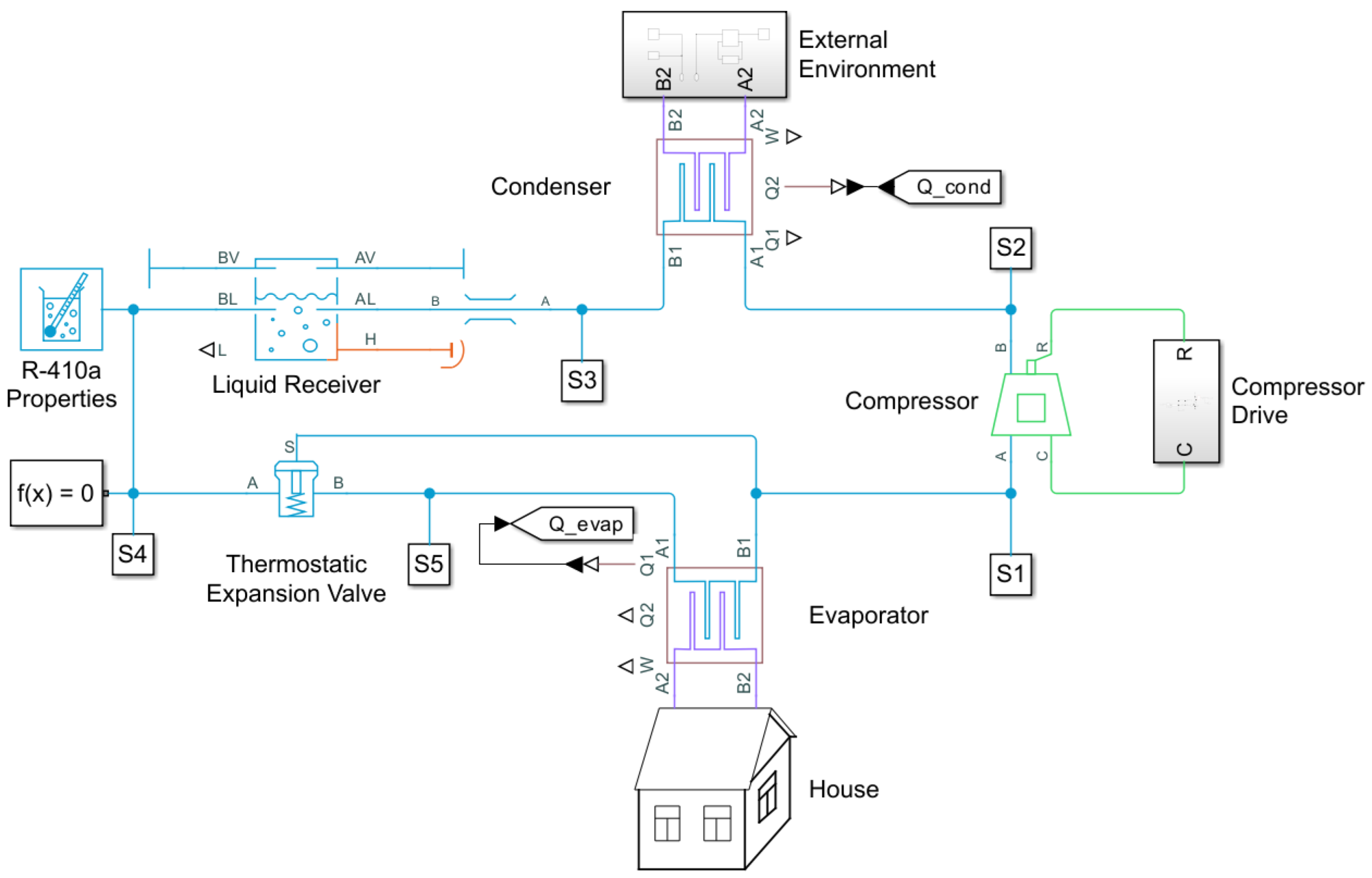
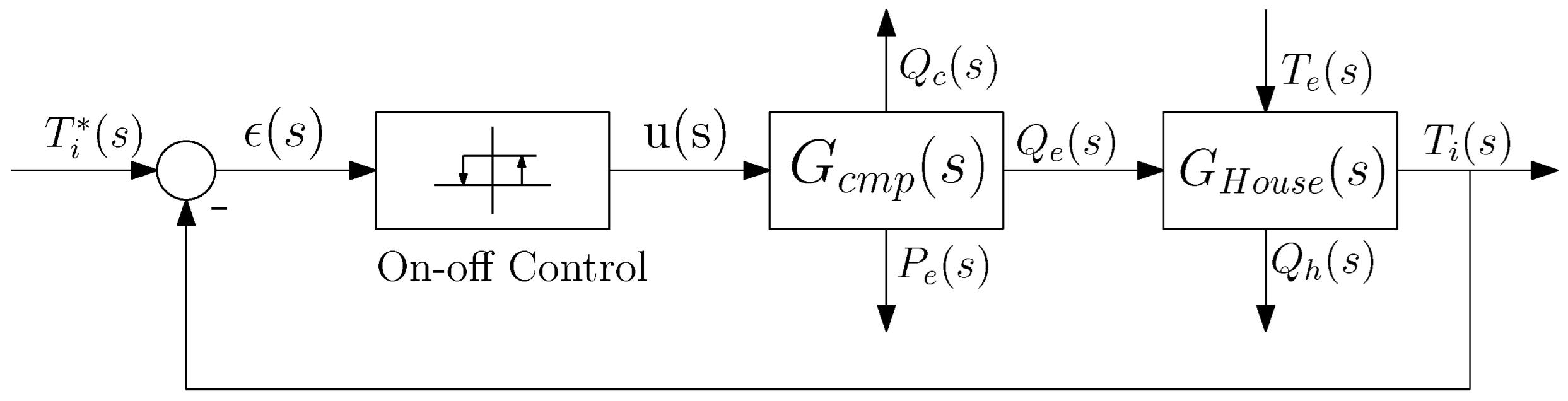
Manufacturers of air handling units require scalable methods to model the thermal behavior of HVAC systems and buildings. A modeling example of a typical residential environment is implemented in the SimScape environment [17]. This model is used as simulation environment to test the control methods presented in the paper. The block diagram of the closed-loop control system is shown in Figure 1. The system is composed of three main parts. First, the measured indoor temperature is compared with the reference temperature to generate an error signal, which is then processed by the controller $c\left(s\right)$. Second, the controller output $u\left(s\right)$ modulates the compressor dynamics $G_{cmp}\left(s\right)$, directly affecting the cooling capacity $Q_e\left(s\right)$ and the power consumption $P_e\left(s\right)$. Finally, these actions interact with the house dynamics $G_{House}\left(s\right)$, where external factors such as the outdoor temperature $T_e\left(s\right)$ further influence the overall thermal behavior. This integrated structure forms a closed-loop system that maintains the desired indoor thermal conditions in a residential environment.

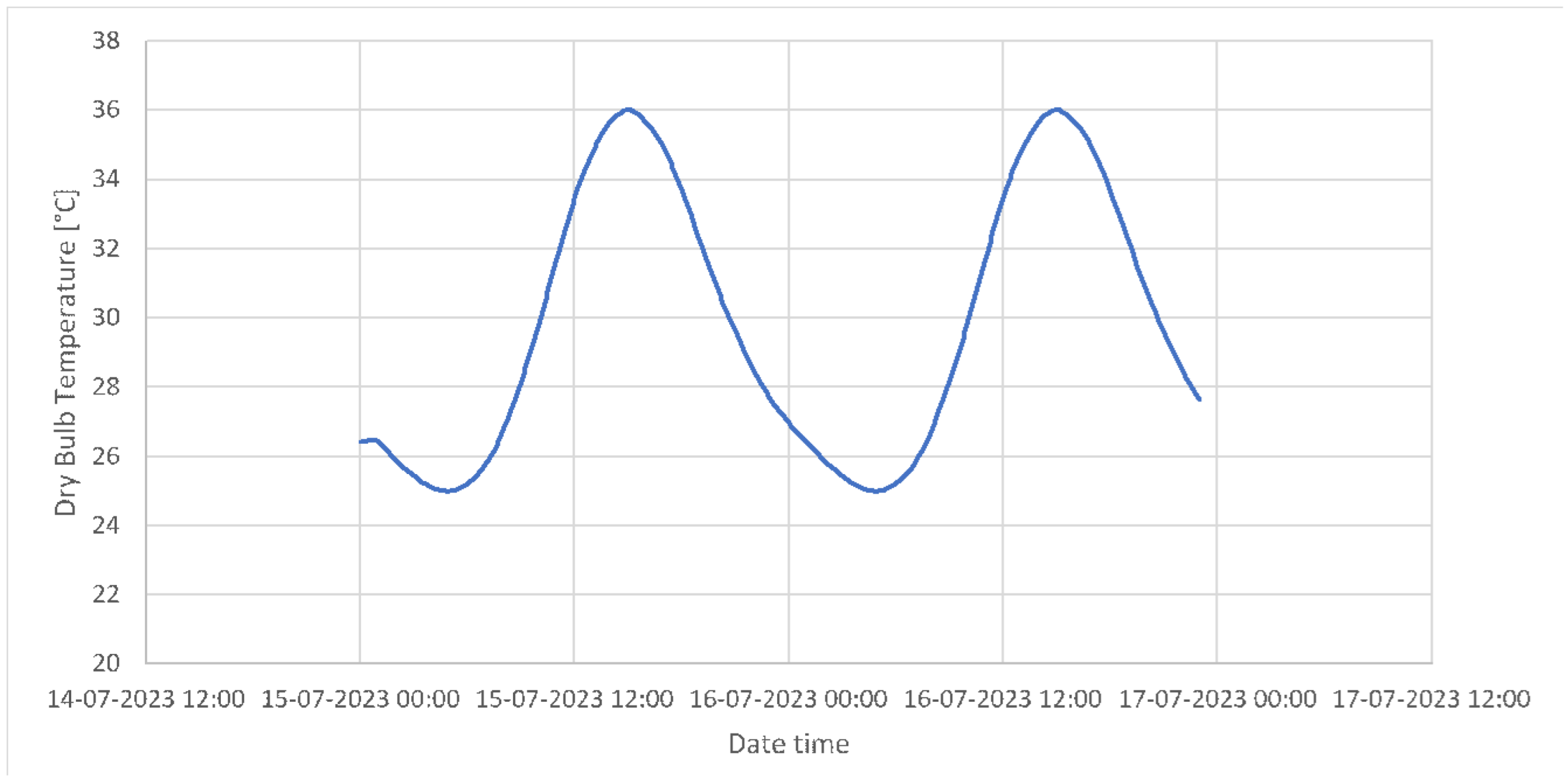
The model parameters are based on a specific air conditioner with known geometric and thermal characteristics. The model is tested in steady-state conditions using the calculation algorithm of the balance of powers shown in [18]. The algorithm presented in [18] is referred by the acronym ASHPC and is used for system component dimensioning. A weather data file is created from the program made available by the National Institute of Standards and Technology (NIST) [19] by specifying the data for the dates 15 and 16 July 2023 for the city of Tirana, Albania. The plot of the generated temperatures is shown in the Figure 2.

The command signal of the compressor is in the interval [0.23–1]. As shown in Figure 3, the system outputs exhibit smooth, non-oscillatory dynamics, supporting the use of low-order ARX models.

The system has two inputs:

1.

compressor speed, $U_c$ expressed in the interval [0.23–1], where 1 refers to the maximum speed of the compressor 120 (rps) and 0.23 refers to the minimum acceptable speed of the compressor 30 (rps).

2.

outdoor temperature, $T_e$ (°C)

and 5 outputs:

1.

indoor temperature, $T_i$ (°C)

2.

power input, $P_e$ (kW)

3.

thermal power, $Q_c$ (kW)

4.

cooling power, $Q_e$ (kW)

5.

house thermal capacity, $Q_h$ (kW)

The only manipulable input of the system is the compressor speed. Having as a reference the model in SimScape and the profile of the external temperature, the system is simulated with a step input and the maximum amplitude. Using the same dataset, the ASHPC algorithm is used to compute the steady-state values of the system state and output [18].

Table 1. ASHPC vs. SimScape calculation.

		ASHPC	SimScape	Error (%)
$$\begin{gathered} T_{in}=27.5{(}^{\circ }\mathrm{C}) \\ {T}_{out}=36{(}^{\circ }\mathrm{C}) \end{gathered}$$	Thermal power (kW)	10.16	10.19	0.3
	Cooling power (kW)	7.6	9.02	18.7
	Input power (kW)	2.56	1.96	23.44
$$\begin{gathered} T_{in}=21.64{(}^{\circ }\mathrm{C}) \\ {T}_{out}=28.55{(}^{\circ }\mathrm{C}) \end{gathered}$$	Thermal power (kW)	9.12	8.71	4.49
	Cooling power (kW)	7.01	7.6	8.416
	Input power (kW)	2.1	1.88	10.476
$$\begin{gathered} T_{in}=20.92{(}^{\circ }\mathrm{C}) \\ {T}_{out}=25{(}^{\circ }\mathrm{C}) \end{gathered}$$	Thermal power (kW)	9.05	8.59	5.08
	Cooling power (kW)	7.17	7.46	4.04
	Input power (kW)	1.89	1.88	0.53
$$\begin{gathered} T_{in}=22.98{(}^{\circ }\mathrm{C}) \\ {T}_{out}=33.77{(}^{\circ }\mathrm{C}) \end{gathered}$$	Thermal power (kW)	9.23	9.137	1
	Cooling power (kW)	6.87	7.98	16.15
	Input power (kW)	2.38	1.91	19.75
$$\begin{gathered} T_{in}=22.34{(}^{\circ }\mathrm{C}) \\ {T}_{out}=27.38{(}^{\circ }\mathrm{C}) \end{gathered}$$	Thermal power (kW)	9.28	8.84	4.74
	Cooling power (kW)	7.23	7.69	6.36
	Input power (kW)	2.06	1.89	8.25

shows the comparison between the dimensioning algorithm and the model in the Simscape environment.

3.1. Model Validation Discrepancies

The iterative performance-validation algorithm by Daci and Bundo [18] employs manufacturer-provided DLLs and a polynomial compressor model, both of which are calibrated against laboratory test data. These components inherently introduce modeling errors due to fitting tolerances. In contrast, the Simscape model uses generic physical parameters—particularly for the heat exchanger—that approximate, but do not exactly replicate, the manufacturer’s specifications. As a result, steady-state outputs such as cooling capacity and input power can differ by up to 20%. These deviations are acceptable for controller design because:

• The ASHPC algorithm performs a static calculation and does not capture the transient dynamics of the heat pump, whereas the Simscape model inherently includes system dynamics critical for control.
• Simscape parameters can be further tuned to reduce steady-state errors if a closer match to the DLL-based performance is required.
• Air conditioning control carries minimal safety risk, so a model that accurately describes dynamic trends—despite moderate static offsets—is sufficient for improving control performance.

3.2. System Identification and Model Selection

To enable the application of Model Predictive Control, a discrete-time model of the system is identified based on data generated by the high-fidelity Simscape model. We adopted the AutoRegressive with eXogenous input (ARX) structure for system identification, due to its simplicity, interpretability, and compatibility with real-time control [16]. The system identification is performed using the Simscape model shown in Figure 4.

Referring to [5,6,14,15], it is considered that the identification of the system is performed based on ARX models, as a flexible and scalable approach. Following the formulation in [16], the general difference equation for a single input–single output (SISO) system is as follows:

$$\begin{array}{c}\hfill y\left(t\right)+k_{1}y(t-1)+\cdots +k_{na}y(t-n_a)=\\ \hfill m_{1}u(t-1)+\dots m_{nb}u(t-n_b)+e\left(t\right)\end{array}$$

(1)

Using shift operator $z^{-1}$ we have that $y(t-n)=z^{-n}y\left(t\right)$. Thus, we can write:

$$\begin{array}{cc}\hfill A\left(z\right)& =1+k_1{z}^{-1}+\cdots +k_{na}{z}^{-na}\hfill \\ \hfill B\left(z\right)& =m_1{z}^{-1}+\cdots +m_{nb}{z}^{-nb}\hfill \\ \hfill G\left(z\right)& ={\displaystyle \frac{B\left(z\right)}{A\left(z\right)}}F\left(z\right)={\displaystyle \frac{1}{A\left(z\right)}}\hfill \\ \hfill y\left(t\right)& =G\left(z\right)u\left(t\right)+F\left(z\right)e\left(t\right)\hfill \end{array}$$

(2)

In matrix form for our system we have:

$$\begin{array}{cc}\hfill \left[\begin{array}{c}{T}_i\\ P_e\\ Q_c\\ Q_e\\ Q_h\end{array}\right]& =\underset{A_m}{\underbrace{\left[\begin{array}{ccccc}{A}_{11}\left(z\right)& A_{12}\left(z\right)& A_{13}\left(z\right)& A_{14}\left(z\right)& A_{15}\left(z\right)\\ A_{21}\left(z\right)& A_{22}\left(z\right)& A_{23}\left(z\right)& A_{24}\left(z\right)& A_{25}\left(z\right)\\ A_{31}\left(z\right)& A_{32}\left(z\right)& A_{33}\left(z\right)& A_{34}\left(z\right)& A_{35}\left(z\right)\\ A_{41}\left(z\right)& A_{42}\left(z\right)& A_{43}\left(z\right)& A_{44}\left(z\right)& A_{45}\left(z\right)\\ A_{51}\left(z\right)& A_{52}\left(z\right)& A_{53}\left(z\right)& A_{54}\left(z\right)& A_{55}\left(z\right)\end{array}\right]}}\left[\begin{array}{c}{T}_i\\ P_e\\ Q_c\\ Q_e\\ Q_h\end{array}\right]\hfill \\ & +\underset{B_m}{\underbrace{\left[\begin{array}{cc}{B}_{11}\left(z\right)& B_{12}\left(z\right)\\ B_{21}\left(z\right)& B_{22}\left(z\right)\\ B_{31}\left(z\right)& B_{32}\left(z\right)\\ B_{41}\left(z\right)& B_{42}\left(z\right)\\ B_{51}\left(z\right)& B_{52}\left(z\right)\end{array}\right]}}\left[\begin{array}{c}{U}_c\\ T_e\end{array}\right]\hfill \\ \hfill & +\underset{e}{\underbrace{\left[\begin{array}{c}{e}_1\\ e_2\\ e_3\\ e_4\\ e_5\end{array}\right]}}\hfill \end{array}$$

(3)

Similar for the case multi input–multi output (MIMO) we have:

$$\begin{array}{c}\hfill G\left(z\right)=A_m^{-1}\left(z\right)B_m\left(z\right)F\left(z\right)=A_m^{-1}\left(z\right)\end{array}$$

(4)

For the multi-input, multi-output (MIMO) case, we identified separate ARX models for each output using the two inputs: compressor speed $U_c$ and outdoor temperature $T_e$. A 48-h simulation profile was used to generate the data, which was split into 70% for training and 30% for testing.

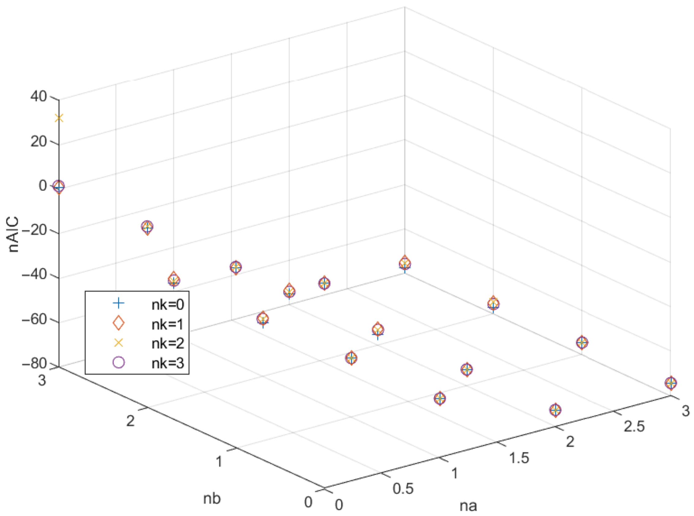
To determine the best model order, a grid search was performed over:

$$n_a,n_b,n_k\in \{0,1,2,3\}$$

Each candidate model was evaluated using three performance metrics:

• Final Prediction Error (FPE),
• Normalized Akaike Information Criterion (nAIC),
• Average FIT on test data.

The results for the top-performing models are summarized in

Table 2. ARX Model Evaluation Summary.

Model (${\mathit{n}}_{\mathit{a}},{\mathit{n}}_{\mathit{b}},{\mathit{n}}_{\mathit{k}}$)	FPE ($·{10}^{-34}$)	nAIC	Average FIT (%)
(2, 2, 0)	2.1	−75.33	87.22
(3, 3, 0)	1.8	−77.68	85.90
(2, 3, 0)	2.3	−73.22	84.10
(1, 2, 0)	3.1	−70.50	81.25

.

Although the ARX(3, 3, 0) model achieved the best FPE and nAIC scores, the ARX(2, 2, 0) model was selected due to its superior prediction FIT on indoor temperature and power consumption—the two variables most critical to control. Moreover, ARX(2, 2, 0) exhibited lower complexity and improved generalization on the 30% held-out test data. This trade-off reflects a standard model selection principle: prioritizing practical control-relevant accuracy over marginal statistical gains.

Figure 5 represents the relation of FPE with the $n_a, n_b, n_k$ parameters. What is noticed is that the FPE does not depend on the $n_k$ parameter. Similarly, Figure 6 represents the relation of nAIC with $n_a, n_b, n_k$. Even in this case, we confirm that the parameter $n_k$ does not influence the value of nAIC. Looking for the minimum value of FPE and nAIC, it results that the minimum FPE is reached for $n_a=3, n_b=3, n_k=0$ and has a value of $1.8·{10}^{-34}$. Meanwhile, the minimum value of nAIC is $-77.68$ and is reached for the same parameter values as FPE.

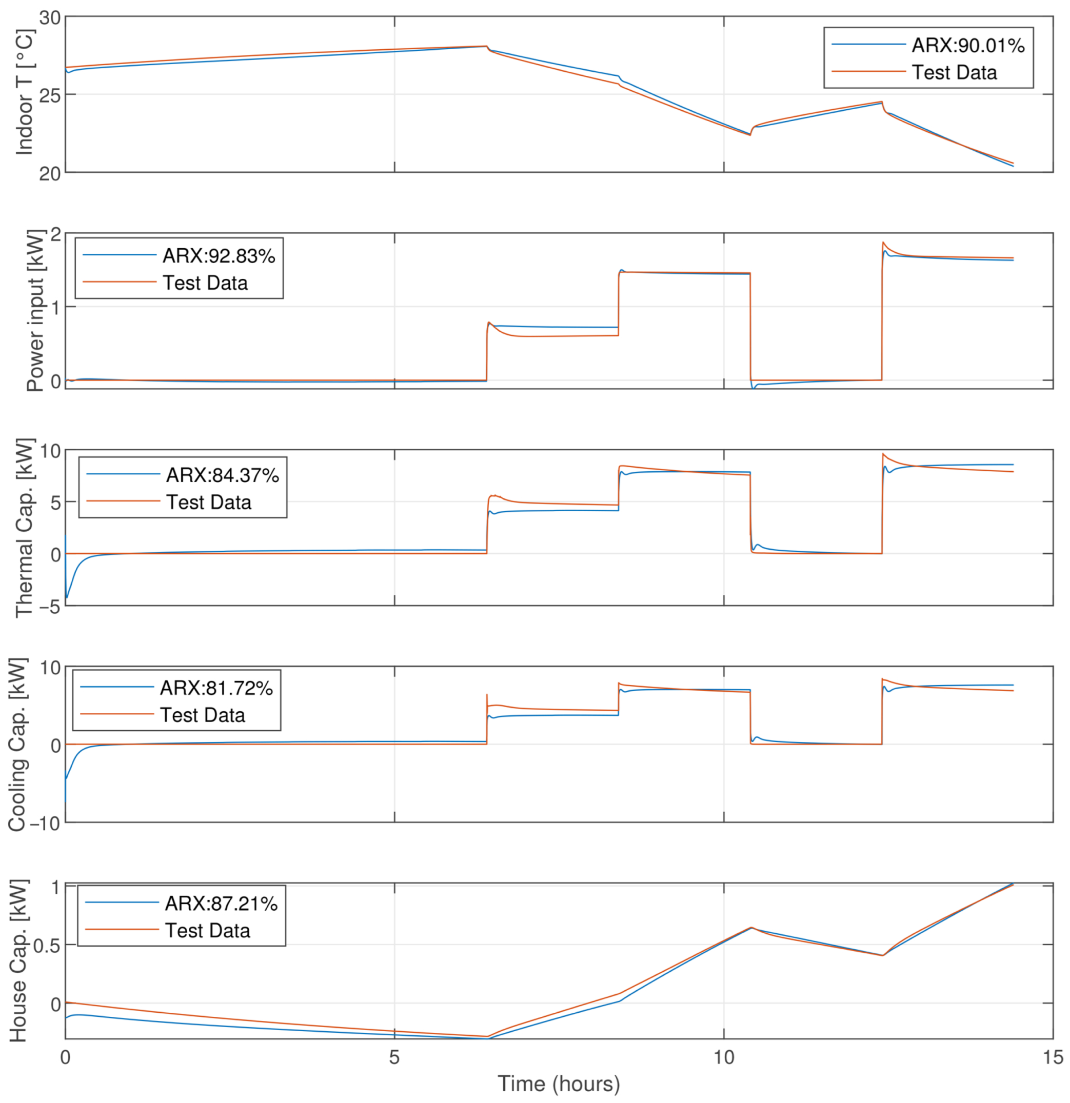
The performance of the ARX(3, 3, 0) model is presented in Figure 7. The plot shows that, except indoor temperature, all the other parameters of the system are described with high or relatively high accuracy. The third performance metric is the average prediction FIT across all outputs. The ARX(2, 2, 0) model gives the best average FIT with the value of 87.22%. The prediction of the system outputs and the FIT for each of them is shown in Figure 8.

We noticed that the prediction FIT of the internal temperature and the power consumption is over 90%. These two variables—indoor temperature and power consumption—are the primary targets of the control system, where the temperature is the controlled variable and the input power is the variable that should be minimized. In these conditions, the accepted model is ARX(2, 2, 0). Since for the design of the control system one of the most widespread forms is the state space, we are presenting the conversion to discrete state space (5) of the ARX(2, 2, 0) in Appendix A.1.

$$\begin{array}{cc}\hfill x(t+T_s)& =Ax\left(t\right)+Bu\left(t\right)+Ke\left(t\right)\hfill \\ \hfill y\left(t\right)& =Cx\left(t\right)+Du\left(t\right)+e\left(t\right)\hfill \end{array}$$

(5)

4. Classical Control Strategies

4.1. On-Off Control

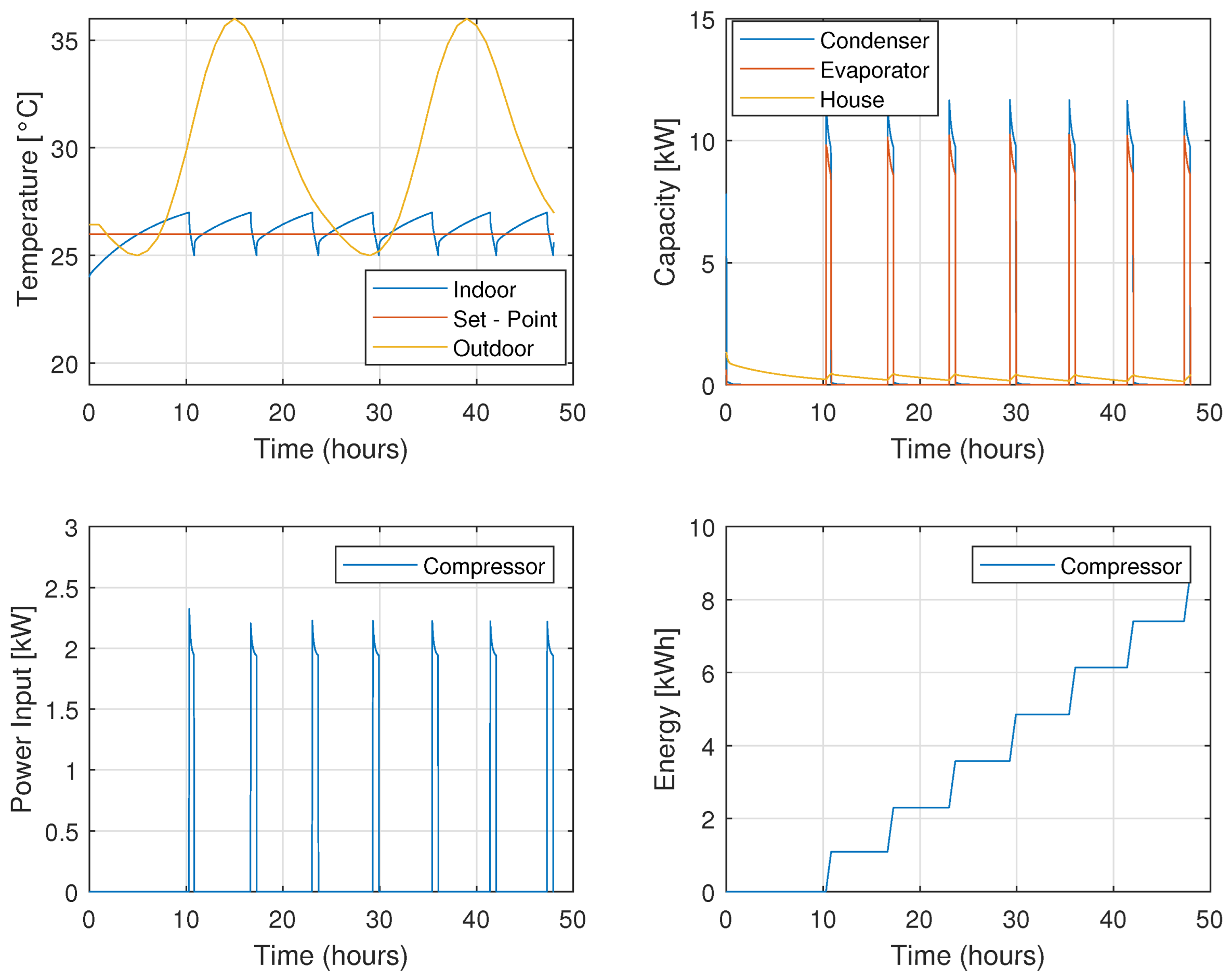
On–Off control remains one of the simplest and most widely used strategies for residential HVAC systems due to its ease of implementation and low cost. As shown in Figure 9, the system activates when the indoor temperature exceeds an upper threshold and deactivates when it falls below a lower limit.

For this study, the indoor temperature was controlled within a hysteresis band of $[25{(}^{\circ }\mathrm{C}),27{(}^{\circ }\mathrm{C})]$ , centered around the recommended summer set-point of $26{(}^{\circ }\mathrm{C})$ [20]. Simulation was conducted using the same 48-h outdoor temperature profile from the NIST dataset. The variables monitored in the simulation are:

1.

Indoor temperature

2.

Thermal capacity

3.

Cooling capacity

4.

Power input

5.

Energy consumption

Figure 10 shows system behavior over the simulation period. The compressor cycles between its minimum and maximum states (0 and 1) depending on the temperature thresholds. The average power consumption over the 48-h period was 0.0502 kW.

4.2. PI Control

4.2.1. PI with Fixed Set-Point and Hysteresis

Many HVAC manufacturers implement PI control using empirical tuning methods. In this approach, the controller maintains the indoor temperature within a predefined comfort range, similar to the On–Off case, but with smoother actuation (Figure 11). The compressor does not operate at full capacity unless required, reducing energy usage.

Figure 12 illustrates the system response under this configuration. The average power consumption dropped to 0.0381 kW—representing a 23.8% reduction compared to the On–Off controller—while maintaining similar comfort levels.

4.2.2. PI with Variable Set-Point

In this variation, the temperature set-point dynamically adjusts based on outdoor temperature. Drawing from EN standards [20], the indoor comfort range during summer is defined as $[25{(}^{\circ }\mathrm{C}),28{(}^{\circ }\mathrm{C})]$. Here, the set-point is updated to maintain an indoor temperature approximately 5 (°C) below the outdoor temperature, bounded between $24{(}^{\circ }\mathrm{C})$ and $27{(}^{\circ }\mathrm{C})$ to ensure comfort. Figure 13 presents the simulation results. Although responsive, this strategy led to increased energy usage (average power: 0.0732 (kW)) due to overcooling during periods of rapidly rising outdoor temperatures.

It is evident that there is an area in which the outside temperature is decreasing and the system continues to be active. To optimize consumption, the air conditioning system will not be activated if the outside temperature is lower or within the set-point range, applying what is known as free-cooling.

4.2.3. PI with Variable Set-Point and Gradient Logic

To mitigate unnecessary energy use during periods of declining outdoor temperature, a supervisory gradient and shutdown rule is added on top of the PI controller. If the external temperature is falling and expected to enter the comfort band, cooling is disabled to exploit passive thermal dynamics (“free-cooling”). Let us

$$\Delta T_{\mathrm{margin}}=3 °\mathrm{C},g_T\left(k\right)={\displaystyle \frac{T_{\mathrm{ext}}\left(k\right)-T_{\mathrm{ext}}(k-1)}{T_s}},$$

and define the Boolean flags

$${\sigma }_T\left(k\right)=\left\{\begin{array}{cc}1,\hfill & T_{\mathrm{ext}}\left(k\right)-\Delta T_{\mathrm{margin}}\le T_{\mathrm{set},\max },\hfill \\ 0,\hfill & \mathrm{otherwise},\hfill \end{array}\right.{\sigma }_g\left(k\right)=\left\{\begin{array}{cc}1,\hfill & g_T\left(k\right)<0,\hfill \\ 0,\hfill & \mathrm{otherwise}.\hfill \end{array}\right.$$

These yield the shutdown indicator

$$\mathrm{off}\_\mathrm{flag}\left(k\right)={\sigma }_T\left(k\right)\wedge {\sigma }_g\left(k\right),$$

and the final compressor command

$$u\left(k\right)=\left\{\begin{array}{cc}0,\hfill & \mathrm{off}\_\mathrm{flag}\left(k\right)=1,\hfill \\ u_{\mathrm{PI}}\left(k\right),\hfill & \mathrm{otherwise},\hfill \end{array}\right.$$

where $u_{\mathrm{PI}}\left(k\right)$ is the output of the PI law and $T_s$ the sampling period.

Figure 14 demonstrates system performance with gradient-aware PI control. Average power consumption dropped to 0.0588 (kW)—an improvement over variable set-point control without gradient logic, though still higher than fixed set-point PI. We notice that we have a considerable improvement compared to the case when we did not consider the gradient; however, this value is close to the average power of the two-position control. Thus, the PI controller with fixed set point and hysteresis effect will give the best performance in terms of comfort and consumption.

5. Advanced Control Strategies

5.1. Model Predictive Control (MPC) Design

5.1.1. Plant Model in Discrete State–Space

Starting from the ARX(2, 2, 0) identification (Appendix A.1), we write the HVAC dynamics in discrete time with sampling period $T_s$:

$$\begin{array}{cc}\hfill x(k+1)& =Ax\left(k\right)+Bu\left(k\right)+Ed\left(k\right),\hfill \end{array}$$

(6)

$$\begin{array}{cc}\hfill y\left(k\right)& =Cx\left(k\right)+Du\left(k\right).\hfill \end{array}$$

(7)

Here $x\in {\mathbb{R}}^n$ is the state vector (thermal states), $u\in {\mathbb{R}}^m$ the manipulated variable (compressor speed), $d\in {\mathbb{R}}^p$ the disturbance (outdoor temperature), and $y\in {\mathbb{R}}^p$ the controlled output (indoor temperature). Equations (6) and (7) form the predictive model used by MPC to forecast future room temperatures [21].

Matrix A describes internal thermal dynamics, B maps control to state change, E accounts for external disturbances, and $C,D$ define the measured output. The fidelity of these matrices directly affects MPC performance [22].

5.1.2. Finite–Horizon Prediction

Over a prediction horizon $N_p$, we define:

$$Y=\left[\begin{array}{c}y(k+1|k)\\ ⋮\\ y(k+N_p|k)\end{array}\right],\Delta U=\left[\begin{array}{c}\Delta u\left(k\right|k)\\ ⋮\\ \Delta u(k+N_c-1|k)\end{array}\right],\Delta u\left(j\right|k)=u\left(j\right|k)-u(j-1|k).$$

Then the multi-step prediction can be written as [21]:

$$Y=Fx\left(k\right)+\mathrm{\Phi }\Delta U+\Gamma U(k-1)+\mathrm{\Psi }D,$$

(8)

where $\mathrm{\Phi }$ maps future input increments to outputs, F is the free response, $\mathrm{\Gamma }$ captures past input effects, and $\mathrm{\Psi }$ includes disturbance forecasts.

Equation (8) linearly relates future outputs to current state, future control moves, past inputs, and known disturbances, providing the basis for optimization [23].

5.1.3. Quadratic Cost Function

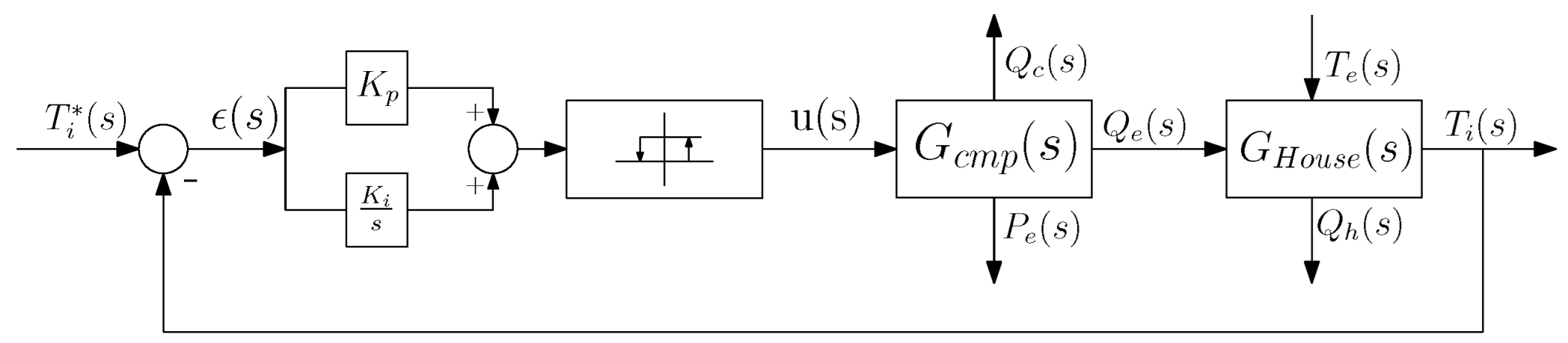
The MPC cost over the horizon is

$$\begin{array}{cc}\hfill J=& {(Y-R)}^T{Q}_y(Y-R)+\Delta U^T{R}_u\Delta U\hfill \\ \hfill & +{\left(U(k-1+N_c)-U(k-1)\right)}^T{R}_{\Delta u}\left(U(k-1+N_c)-U(k-1)\right),\hfill \end{array}$$

(9)

where R is the stacked reference trajectory, $Q_y⪰0$ weights output tracking error, $R_u⪰0$ penalizes control moves, and $R_{\Delta u}⪰0$ penalizes the terminal move [21].

The first term enforces adherence to the set-point or comfort band. The second limits aggressive actuator changes. The terminal term shapes end-of-horizon behaviour and can improve closed-loop stability [23].

5.1.4. Constraints

Subject to

$$\begin{array}{cc}{u}_{min}\hfill & \le u(k+i|k)\le u_{max},i=0,\dots ,N_c-1,\hfill \end{array}$$

(10)

$$\begin{array}{cc}{y}_{min}\hfill & \le y(k+j|k)\le y_{max},j=1,\dots ,N_p,\hfill \end{array}$$

(11)

with in our HVAC case:

$$0.23\le u\le 1.0,{25}^{\circ }\mathrm{C}\le y\le {28}^{\circ }\mathrm{C}.$$

These constraints guarantee both physical actuator limits and occupant comfort boundaries [22].

5.1.5. QP (Quadratic Problem) Formulation and Receding Horizon

Combining (8) and (9), the optimization becomes a quadratic program:

$$\begin{array}{cc}\hfill \underset{\Delta U}{min}& \frac{1}{2}\Delta U^{\mathsf{T}}H\Delta U+f^{\mathsf{T}}\Delta U,\hfill \\ \hfill \mathrm{s}.\mathrm{t}.& M\Delta U\le b,\hfill \end{array}$$

(12)

where

$$H=2\left({\mathrm{\Phi }}^{\mathsf{T}}{Q}_y\mathrm{\Phi }+R_u\right),f=2{\mathrm{\Phi }}^{\mathsf{T}}{Q}_y\left(Fx\left(k\right)+\mathrm{\Gamma }U(k-1)+\mathrm{\Psi }D-R\right),$$

and $M,b$ encode (10) and (11) in terms of $\Delta U$.

• Implementation Strategy

At each control interval:

1.

Measure the current state $x\left(k\right)$ and retrieve disturbance forecast D.

2.

Solve the QP (12) for optimal $\Delta U^{*}$.

3.

Apply $u\left(k\right)=u(k-1)+\Delta u\left(k\right|k)$.

4.

Repeat in the next interval (receding horizon).

The ability to include disturbance forecasts D (e.g., outdoor temperature trend) in (8) provides a feed-forward action that enhances performance over purely feedback controllers [21].

5.2. Model Predictive Control Implementation

For the implementation of predictive control, the model shown in the Equation (5) is used. The cost function used is the standard MPC cost function shown in (9). The parameter of the applied MPC are shown in

Table 3. MPC tuning parameters used in the simulations.

Parameter	Symbol	Value
Sampling period	$T_s$	600 s
Prediction horizon	$N_p$	5
Control horizon	$N_c$	1
Output-tracking weight	$Q_y$	0.7
Manipulated-variable weight	$R_u$	10
Manipulated-rate ($\Delta$u) weight	$R_{\Delta u}$	0.15
Manipulated variable constraints (min / max)	$u_{min},u_{max}$	0.23, 1.0

. For the application of the MPC there are two basic approaches:

1.

Consider that reference and disturbance signals do not change their value in the prediction horizon

2.

Preview the values of reference and disturbance signals over the prediction horizon

Knowing that the external temperature is constantly changing, we adopt the full preview approach and empirically tune the MPC parameters. The tuning prioritizes a balance between look-ahead capability, computational tractability, and actuator smoothness, which is particularly suitable for this slow-dynamics HVAC system.

Similar to the case of the PI controller analyzed in Section 4.2, two approaches have been considered. In the first approach, the external temperature gradient is not considered, while in the second approach it is considered. It is important to emphasize that prior knowledge of the external temperature is fundamental for the application of MPC, therefore there would be no added difficulties for the application of the approach that considers the gradient of the external temperature.

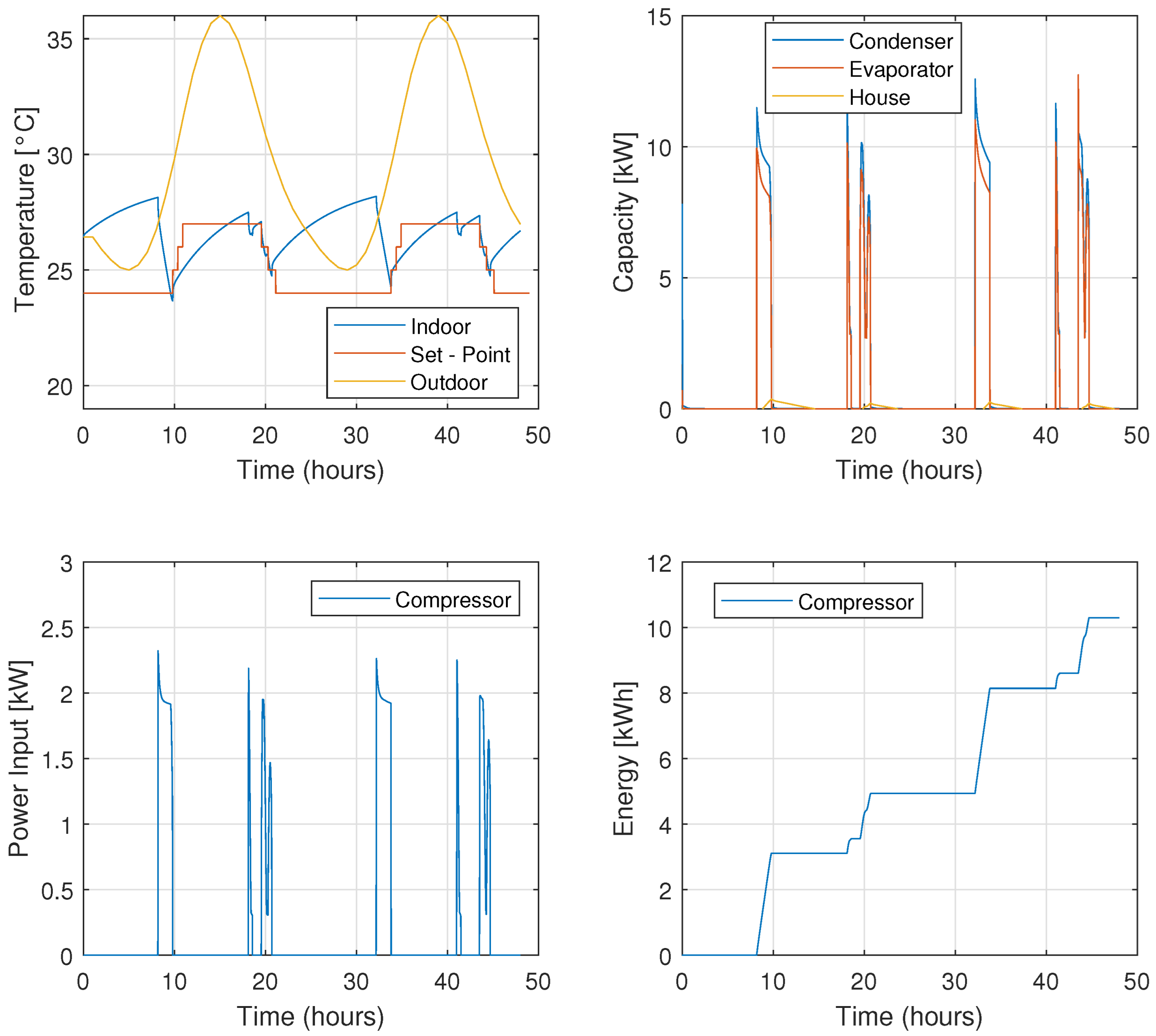
In Figure 15, we have presented plots indicating the performance of the system when the control algorithm includes only the MPC. The average power of the system is 0.0305 kW. This value turns out to be about 19.95% less than the most efficient scenario seen so far. The temperature of the internal environment is all the time within the acceptable range and the control variable does not present aggressive behavior. In other words, we can say that in terms of comfort and aggressiveness we are in optimal conditions and that the application of the MPC made the savings increase by around 20% compared to the most effective of the classic methods.

5.2.1. Note on Outdoor-Temperature Forecasting

In all our MPC simulations we assume “ideal” knowledge of the outdoor temperature over the full prediction horizon, by simply replaying the recorded 15–16 July 2023 Tirana weather profile as if it were a perfect forecast. This permits us to isolate the intrinsic benefit of including gradient logic in the controller. In practice, publicly available meteorological services (e.g., NOAA, ECMWF, national weather stations) or local on-site sensors combined with short-term statistical predictors can deliver 1–6 h temperature forecasts with root-mean-square errors on the order of 0.5–1.0 °C. Future work will integrate such realistic forecast errors into the simulation pipeline and quantify their impact on both energy savings and comfort.

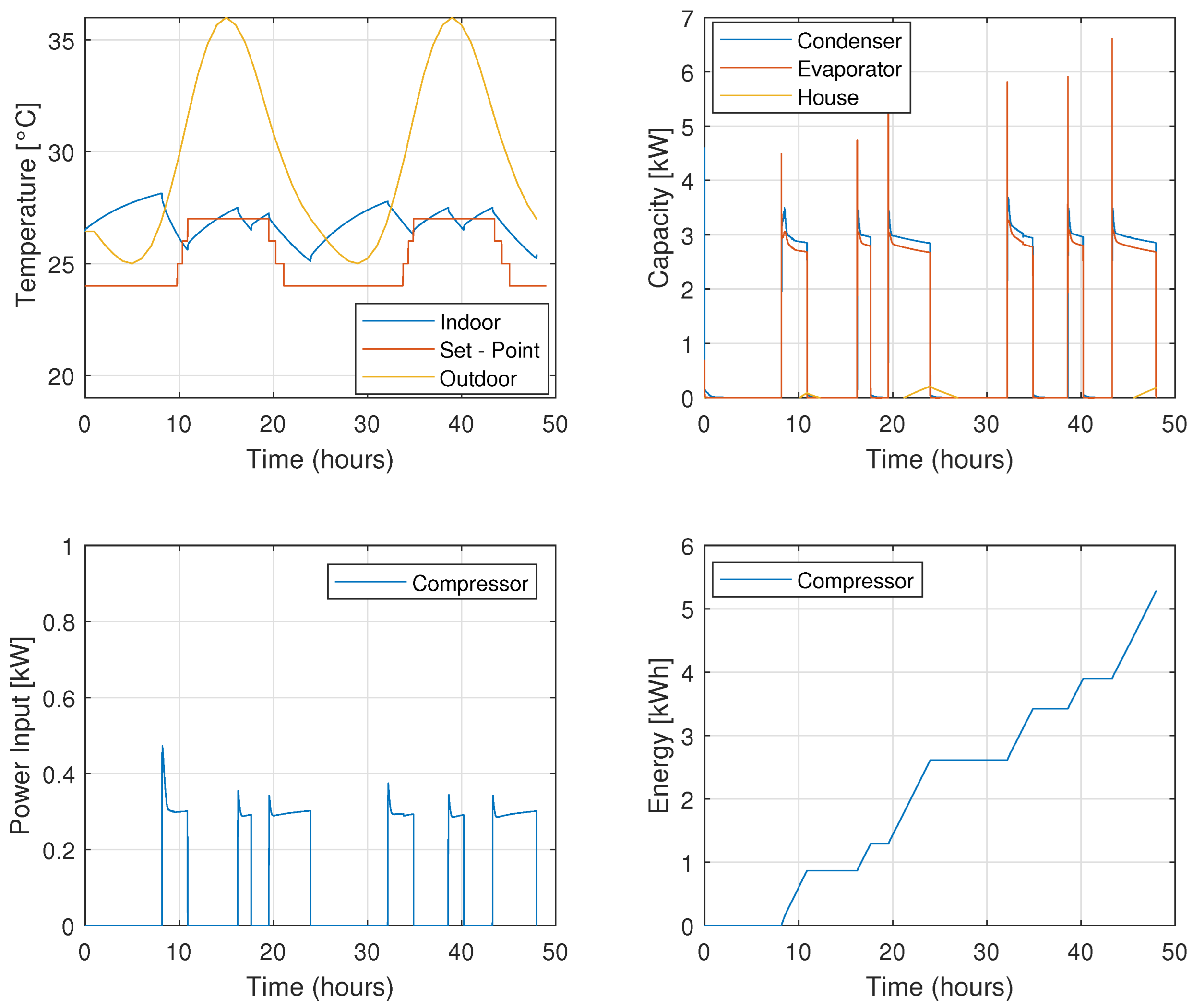
5.2.2. MPC with Outdoor-Temperature Gradient Logic

The baseline MPC is first computed as described in Section 5.1. After solving the QP and applying the control move $u_{\mathrm{MPC}}\left(k\right)$, the compressor signal is then subject to the same supervisory gradient and shutdown logic defined in Section 4.2.3.

Concretely, if

$$\Delta T_e\left(k\right)=T_e^{\mathrm{pred}}\left(k\right|k)-T_e^{\mathrm{pred}}(k-1|k-1)$$

and

$$\Delta T_e\left(k\right)<0\mathrm{and}{T}_e^{\mathrm{pred}}\left(k\right|k)-\delta <T_{max}^{\mathrm{comfort}},$$

then the compressor command is forced to zero:

$$u\left(k\right)=0,$$

otherwise $u\left(k\right)=u_{\mathrm{MPC}}\left(k\right)$.

Here $\delta$ is a tunable threshold balancing energy savings against occupant comfort, and $T_{max}^{\mathrm{comfort}}$ is the upper bound of the desired indoor comfort range. This logic turns off the compressor whenever the forecasted outdoor temperature is falling into a region where indoor comfort can be maintained without active cooling.

The MPC controller preemptively disables the compressor when the outdoor temperature is forecasted to decrease and will remain within 1 °C of the upper comfort limit. This prevents unnecessary energy use and exploits passive thermal dynamics.

Figure 16 shows the performance of the system when, in addition to the effect of the MPC, the external temperature gradient is also considered. In this case, since the controller itself has a predictive effect, it is considered that the controller will turn off when the trend of the external temperature is decreasing and the distance with the largest set-point value is less than or equal to 1. The average power is 0.027 kW. Here we can see that the power is reduced by about 30% compared to the PI controller with hysteresis effect. The temperature plot, shows that the decrease in consumption is accompanied by the deterioration of comfort conditions. However, we can say that this is an acceptable effect because the upper limit is exceeded by $0.173 °$C. Thus, considering the derivative of the external temperature in series with MPC, improves the consumption by about 30% compared to the most used control method that we encounter today in this industry.

5.2.3. MPC Implementation and Real-Time Feasibility

The MPC optimization was implemented using MATLAB’s (2013b) Model Predictive Control Toolbox within Simulink, employing the built-in ‘MPC Controller’ block. Executions were performed on a Windows 11 Pro machine with a 12th Gen Intel^® Core™ i7-1280P CPU (2.00 GHz) and 32 GB of RAM. Simulating the full high-fidelity plant model in Simscape over a 48 h profile took approximately 30 min, whereas running the MPC on the identified discrete state-space model alone completed in about 1 min. The MPC solver itself executes in the millisecond range on this hardware. Since residential HVAC dynamics evolve over timescales of minutes to hours, the solver’s execution time imposes negligible additional delay, demonstrating that real-time deployment on an embedded controller is readily achievable for this application.

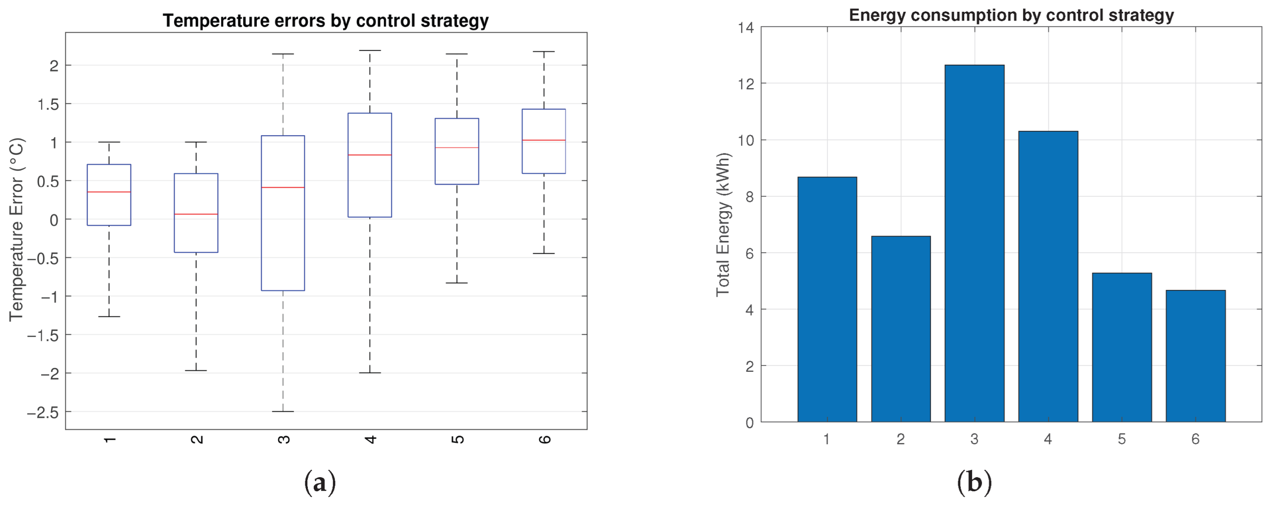
6. Comparative Evaluation of Control Approaches

In this section, we compare the performance of all six control strategies introduced in Section 4 and Section 5. The evaluation focuses on energy consumption, thermal comfort, and control smoothness across a 48-h summer simulation. Each controller was tested under identical external temperature profiles and building conditions.

In

Table 4. Summary of performance metrics across all control strategies over a 48-h summer profile.

ID	Method	Mean Pe (kW)	Mean Tin (°C)	Mean Qc (kW)
1	On-Off	0.0502	26.24	0.9338
2	PI + hysteresis	0.0381	26.03	0.9117
3	PI + variable set-point	0.0732	26.085	1.5164
4	PI + variable set-point + gradient	0.0596	26.67	1.1593
5	MPC	0.0305	26.83	1.0976
6	MPC + gradient	0.0270	26.99	0.9811

Where: Mean $P_e$ (kW) is the electrical power averaged over time, calculated as the total electrical energy consumed (in kWh) in the simulation horizon of 48 h divided by 48 h. The mean $T_{\mathrm{in}}$ (°C) and the mean $Q_c$ (kW) are the corresponding average indoor temperature and thermal power time, respectively, calculated during the same period.

we have shown a summary of data with interest of 6 applied control techniques. It is worth noting that in any case the average internal temperature is within the acceptable range. Two cases of MPC application are the most efficient in terms of consumption. The method that continues to be interesting is the PI control method with hysteresis effect. This method, not at all complex to implement and with a long history, presents an average temperature almost equal to the recommended temperature $26.03°$C. After the optimization technique, this method is the best in terms of comfort and consumption. What is noticed is that the system will perform better in the case when we are dealing with control when the set point is static than when the set point is of the scale type. In terms of implementation, the simplest method would be On-Off. This simplicity translates into a low initial cost, which is accompanied by a consumption almost double that of the optimal method studied and about 32% more than the PI + hysteresis case. The industry today offers numerous electronic solutions that can solve the optimization problem. On the other hand, the market is not always ready to invest in what would be the most effective solution in the long term. Programmable Logic Controllers (PLC) found in the industry today are able to more easily manage a high number of PID controllers. In these conditions, we say that when the initial investment is possible, the application of the MPC method considering the temperature gradient is the most suitable solution. In other conditions, the most effective solution is the application of the PI controller with hysteresis effect with static set point.

Figure 17 and Table 4 jointly illustrate the trade-offs between energy consumption and thermal comfort. Among all strategies, MPC with gradient-based shutdown achieved the lowest energy usage (0.0270 kW average), reducing consumption by nearly 30% compared to the On–Off baseline and by 29% relative to PI with hysteresis.

Notably, while MPC-based methods exhibit slightly higher mean indoor temperatures, these remain well within the allowable comfort band and do not compromise user experience. The PI controller with fixed set-point and hysteresis remains the most efficient among classical methods, striking a strong balance between comfort and simplicity.

PI controllers using variable set-points, particularly without gradient logic, show significantly higher energy consumption due to persistent overcooling during periods of declining outdoor temperature. Incorporating the outdoor temperature gradient into both PI and MPC schemes provides measurable efficiency gains without introducing noticeable thermal discomfort.

Overall, MPC with gradient logic offers the best combination of efficiency and robustness, while the PI + hysteresis controller provides a practical near-optimal solution with minimal implementation complexity. Recommendation: For manufacturers with access to forecast data and moderate computational capabilities, MPC with gradient logic offers the highest performance. For cost-sensitive applications or retrofit scenarios, PI with hysteresis and fixed set-point provides an attractive trade-off between performance and simplicity.

7. Conclusions

This study presented an end-to-end, simulation-based development framework for residential HVAC control design, integrating virtual modeling, system identification, and controller evaluation. A high-fidelity Simscape model, validated against manufacturer DLLs using the Daci–Bundo algorithm, successfully replicated building and heat pump behavior with steady-state errors under 20% and prediction FITs exceeding 90% for key variables such as indoor temperature and power consumption.

From this validated virtual environment, an ARX(2,2,0) model was identified and converted into a discrete-time state-space form suitable for controller synthesis. Six control strategies were designed and benchmarked, including On–Off control, PI with hysteresis, PI with variable set-point (with and without temperature-gradient logic), and two MPC variants.

Simulation results under realistic 48-h summer conditions demonstrated that MPC with outdoor temperature gradient preview achieved the highest efficiency, reducing energy consumption by approximately 30% relative to classical PI control with hysteresis. This was achieved without compromising thermal comfort. Moreover, the MPC solver’s millisecond-level execution time, combined with the slow thermal dynamics of residential buildings, confirms its suitability for real-time embedded implementation.

By eliminating the need for extensive physical prototyping during the early design stages, this virtual-first workflow offers a scalable and cost-effective path for HVAC control development. The findings highlight the strong potential of predictive control—especially gradient-informed MPC—to deliver substantial energy savings in residential applications while preserving user comfort.

7.1. Limitations and Future Work

All results presented are based on simulation using a virtual plant model, which, although validated, does not capture all real-world nonlinearities, disturbances, or hardware limitations. Experimental validation in physical testbeds is necessary to confirm real-world effectiveness and robustness. Future work will involve deploying the proposed MPC strategies in a controlled climatic chamber and in a live residential setting. This will help assess implementation challenges, hardware constraints, model mismatch effects, and user acceptance in practice.

7.2. Experimental Validation Plan

To confirm the real-world performance of the proposed controllers, we plan a two-stage experimental campaign:

1.

Controlled climatic-chamber tests.

• Setup: A small environmental chamber equipped with a residential-scale heat pump, instrumented with temperature and power sensors.
• Procedure: Replicate the same 48 h summer temperature profile used in simulation (via chamber setpoint control), and sequentially run each controller (On–Off, PI variants, MPC variants) for direct energy and comfort comparison.
• Metrics: Record indoor temperature, compressor power, and actuator signals at 1 Hz; compute energy savings and comfort violations using the same indicators defined in simulation.

2.

Pilot residential field test.

• Setup: Retrofit a single-family home with data acquisition (indoor/outdoor temperature, power meter) and a programmable controller (e.g., PLC or embedded PC).
• Procedure: Alternate weekly operation under the baseline PI+hysteresis and our MPC+gradient controllers, while logging identical performance metrics. Outdoor weather forecasts will feed the MPC’s disturbance model.
• Metrics: Compare monthly energy consumption, comfort-band violations, and actuator activity to quantify benefits, robustness to forecast errors, and practical implementation overhead.

This staged approach—first in a fully controlled chamber, then in a real home—will allow us to quantify model mismatch, unmodeled disturbances, and practical implementation issues (forecast errors, communication delays, hardware constraints) before recommending production deployment.

References

- Široký, J.; Oldewurtel, F.; Cigler, J.; Prívara, S. Experimental analysis of model predictive control for an energy efficient building heating system. Appl. Energy 2011, 88, 3079–3087. [Google Scholar] [CrossRef]
- Afram, A.; Janabi-Sharifi, F.; Fung, A.S.; Raahemifar, K. Artificial neural network (ANN) based model predictive control (MPC) and optimization of HVAC systems: A state of the art review and case study of a residential HVAC system. Energy Build. 2017, 141, 96–113. [Google Scholar] [CrossRef]
- Afram, A.; Janabi-Sharifi, F. Supervisory model predictive controller (MPC) for residential HVAC systems: Implementation and experimentation on archetype sustainable house in Toronto. Energy Build. 2017, 154, 268–282. [Google Scholar] [CrossRef]
- Rehrl, J.; Horn, M. Temperature control for HVAC systems based on exact linearization and model predictive control. In Proceedings of the 2011 IEEE International Conference on Control Applications (CCA), Denver, CO, USA, 28–30 September 2011; pp. 1119–1124. [Google Scholar] [CrossRef]
- Royer, S.; Thil, S.; Talbert, T.; Polit, M. Black-box modeling of buildings thermal behavior using system identification. Ifac Proc. Vol. 2014, 47, 10850–10855. [Google Scholar] [CrossRef]
- Merema, B.; Breesch, H.; Saelens, D. Comparison of model identification techniques for MPC in all-air HVAC systems in an educational building. E3S Web Conf. 2019, 111, 01053. [Google Scholar] [CrossRef]
- Vivian, J.; Croci, L.; Zarrella, A. Experimental tests on the performance of an economic model predictive control system in a lightweight building. Appl. Therm. Eng. 2022, 213, 118693. [Google Scholar] [CrossRef]
- Parisio, A.; Fabietti, L.; Molinari, M.; Varagnolo, D.; Johansson, K.H. Control of HVAC systems via scenario-based explicit MPC. In Proceedings of the 53rd IEEE Conference on Decision and Control, Los Angeles, CA, USA, 15–17 December 2014; pp. 5201–5207. [Google Scholar] [CrossRef]
- Avci, M.; Erkoc, M.; Rahmani, A.; Asfour, S. Model predictive HVAC load control in buildings using real-time electricity pricing. Energy Build. 2013, 60, 199–209. [Google Scholar] [CrossRef]
- West, S.R.; Ward, J.K.; Wall, J. Trial Results from a Model Predictive Control and Optimisation System for Commercial Building HVAC. Energy And Build. 2014, 72, 271–279. [Google Scholar] [CrossRef]
- Bengea, S.C.; Kelman, A.D.; Borrelli, F.; Taylor, R.; Narayanan, S. Implementation of model predictive control for an HVAC system in a mid-size commercial building. HVAC&R Res. 2014, 20, 121–135. [Google Scholar] [CrossRef]
- Wang, W.; Hu, B.; Wang, R.Z.; Luo, M.; Zhang, G.; Xiang, B. Model predictive control for the performance improvement of air source heat pump heating system via variable water temperature difference. Int. J. Refrig. 2022, 138, 169–179. [Google Scholar] [CrossRef]
- Parisio, A.; Varagnolo, D.; Molinari, M.; Pattarello, G.; Fabietti, L.; Karl, H. Johansson, Implementation of a Scenario-based MPC for HVAC Systems: An Experimental Case Study. Ifac Proc. Vol. 2014, 47, 599–605. [Google Scholar] [CrossRef]
- Prívara, S.; Cigler, J.; Váňa, Z.; Oldewurtel, F.; Sagerschnig, C.; Žáčeková, E. Building modeling as a crucial part for building predictive control. Energy Build. 2013, 56, 8–22. [Google Scholar] [CrossRef]
- Yun, K.; Luck, R.; Mago, P.J.; Cho, H. Building hourly thermal load prediction using an indexed ARX model. Energy Build. 2012, 54, 225–233. [Google Scholar] [CrossRef]
- Ljung, L. System Identification: Theory for the User; Prentice Hall PTR: Upper Saddle River, NJ, USA, 1999; ISSN 0891-4559. [Google Scholar]
- The MathWorks, Inc. “Refrigeration Cycle (Air Conditioning) Example” mathworks.com. Available online: https://www.mathworks.com/help/hydro/ug/residential-refrigeration-unit.html (accessed on 15 May 2024).
- Daci, A.; Bundo, J. Mathematical model for calculating the equilibrium point of the refrigerant circuit. IOP Conf. Ser. Mater. Sci. Eng. 2020, 909, 012013. [Google Scholar] [CrossRef]
- National Institute of Standards and Technology. HVACSIM20.7. Available online: https://www.nist.gov/services-resources/software/hvac-simulation-plus-other-systems-hvacsim (accessed on 27 August 2024).
- Brelih, N. Thermal and acoustic comfort requirements in European standards and national regulations. Rehva Eur. Hvac J. 2013, 50, 16–19. [Google Scholar]
- Rawlings, J.B.; Mayne, D.Q.; Diehl, M. Model Predictive Control: Theory, Computation, and Design; Nob Hill Publishing: San Francisco, CA, USA, 2009. [Google Scholar]
- Camacho, E.F.; Bordons, C. Model Predictive Control, 2nd ed.; Springer: London, UK, 2013. [Google Scholar]
- Maciejowski, J.M. Predictive Control with Constraints; Prentice Hall: London, UK, 2002. [Google Scholar]
Figure 1.
Control system schematics.
Figure 2.
Outdoor air temperature profile for 15–16 July 2023 (Tirana, Albania).
Figure 3.
System identification data logging with sampling time .
Figure 4.
SimScape virtual model.
Figure 5.
Final Prediction Error (FPE) across ARX model orders .
Figure 6.
nAIC vs. .
Figure 7.
Model ARX(3, 3, 0) performance compared to the 30% of simulated data used for testing.
Figure 8.
Model ARX(2, 2, 0) performance compared to the 30% of simulated data used for testing.
Figure 9.
On-Off control scheme.
Figure 10.
On-Off system performance.
Figure 11.
PI control scheme.
Figure 12.
PI + Hysteresis system performance.