
The Application of KNN-Optimized Hybrid Models in Landslide Displacement Prediction

 ,
,
Abstract
1. Introduction
2. Methodology
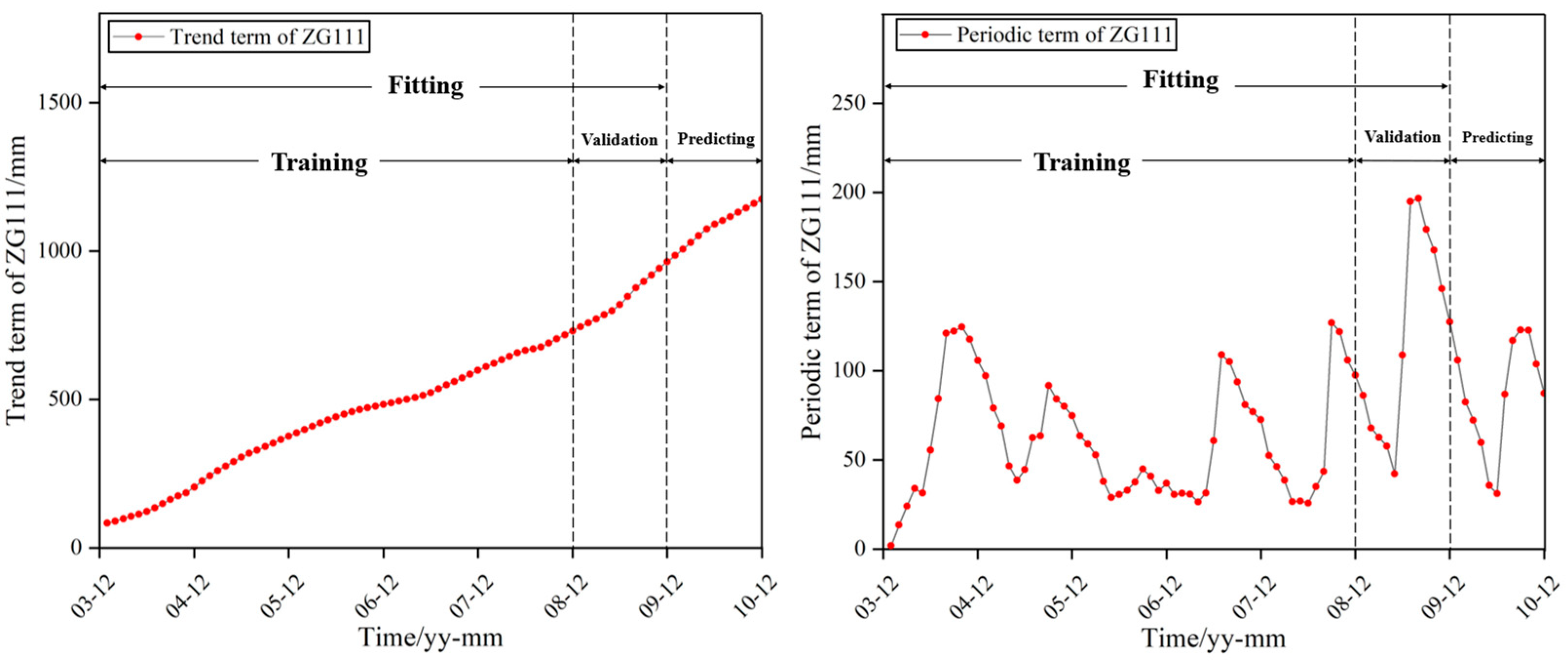
2.1. Separation of Displacement Time Series into Long-Term and Cyclic Patterns
2.2. Moving Average Methods
2.3. Support Vector Regression
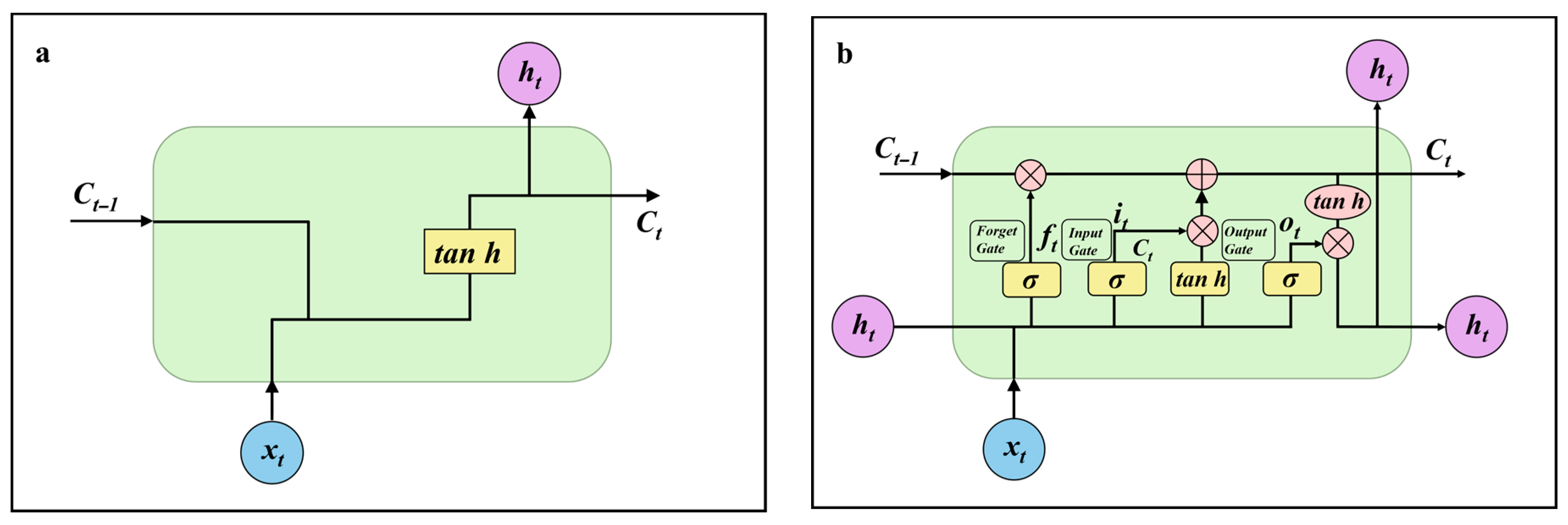
2.4. Long Short-Term Memory Neural Networks
2.5. Reliability Evaluation of the Model
3. Study Site
3.1. Bazimen Landslide
3.2. Landslide Inventory
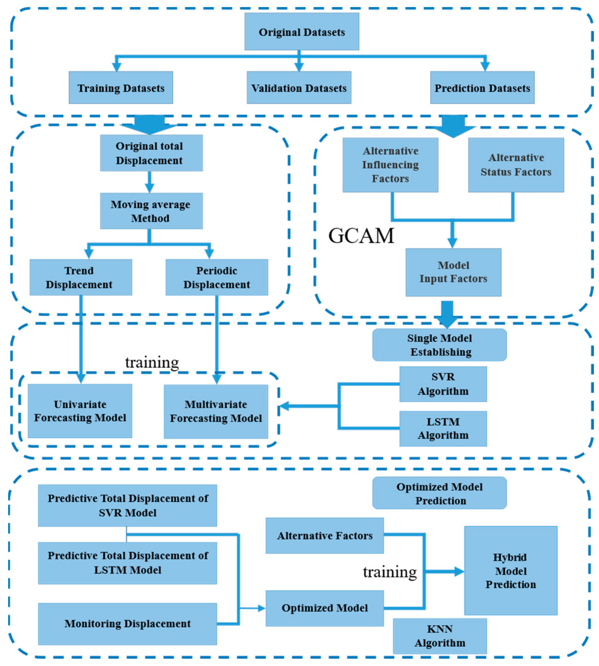
4. Prediction Process
4.1. Point Selection and Data Processing
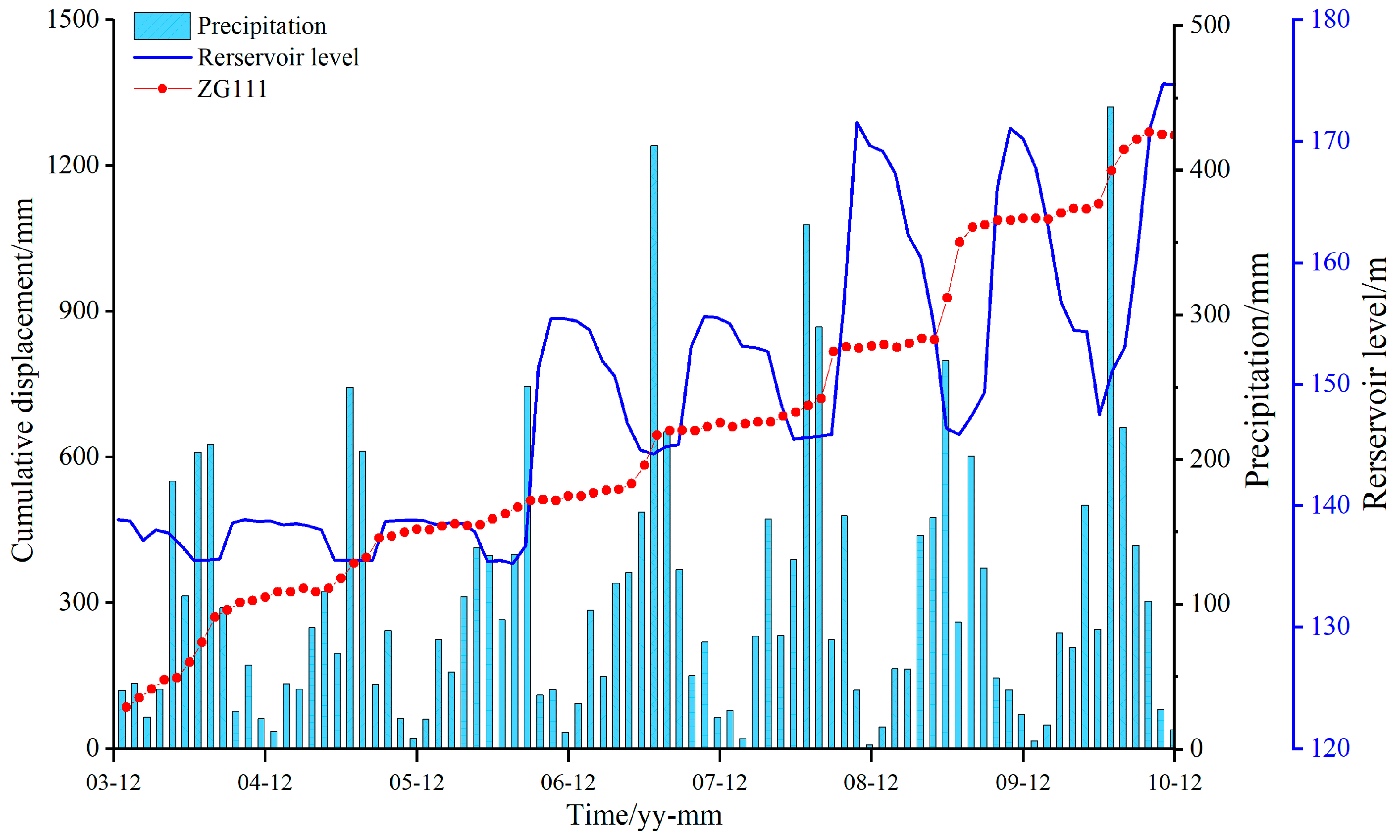
4.2. Factor Selection
4.3. Normalization and Inverse Normalization
4.4. Parameters of SVRs and LSTMs
5. Results
5.1. SVR Models and LSTM Models
5.2. Sequential Hybrid Model Optimized by K-Nearest Neighbor
6. Discussion
7. Conclusions
Author Contributions
Funding
Institutional Review Board Statement
Informed Consent Statement
Data Availability Statement
Acknowledgments
Conflicts of Interest
References
- Zeng, T.; Yin, K.; Jiang, H. Groundwater level prediction based on a combined intelligence method for the Sifangbei landslide in the Three Gorges Reservoir Area. Sci. Rep. 2022, 12, 11108. [Google Scholar] [CrossRef] [PubMed]
- Li, X.; Li, Q.; Wang, Y. Effect of slope angle on fractured rock masses under combined influence of variable rainfall infiltration and excavation unloading. J. Rock Mech. Geotech. Eng. 2024, 16, 4154–4176. [Google Scholar] [CrossRef]
- Xu, J.; Jiang, Y.; Yang, C. Landslide Displacement Prediction during the Sliding Process Using XGBoost, SVR and RNNs. Appl. Sci. 2022, 12, 6056. [Google Scholar] [CrossRef]
- Zhang, J.; Chen, C.; Wu, C. Development of An Image-based Borehole Flowmeter for Real-time Monitoring of Groundwater Flow Velocity and Direction in Landslide Boreholes. IEEE Sens. J. 2024, 24, 42079–42087. [Google Scholar] [CrossRef]
- Zhang, J.; Lin, C.; Tang, H. Input-parameter optimization using a SVR based ensemble model to predict landslide displacements in a reservoir area-A comparative study. Appl. Soft Comput. 2024, 150, 111107. [Google Scholar] [CrossRef]
- Liu, Z.; Guo, D.; Lacasse, S. Algorithms for intelligent prediction of landslide displacements. J. Zhejiang Univ. Sci. A 2020, 21, 412–429. [Google Scholar] [CrossRef]
- Zhang, J.; Tang, H.; Zhou, B. A new early warning criterion for landslides movement assessment: Deformation Standardized Anomaly Index. Bull. Eng. Geol. Environ. 2024, 83, 205. [Google Scholar] [CrossRef]
- Li, D.; Sun, Y.; Yin, K. Displacement characteristics and prediction of Baishuihe landslide in the Three Gorges Reservoir. J. Mt. Sci. 2019, 16, 2203–2214. [Google Scholar] [CrossRef]
- Zhang, J.; Tang, H.; Tan, Q. A generalized early warning criterion for the landslide risk assessment: Deformation probability index (DPI). Acta Geotech. 2024, 19, 2607–2627. [Google Scholar] [CrossRef]
- Jiang, H.; Wang, Y.; Guo, Z. Landslide Displacement Prediction Stacking Deep Learning Algorithms: A Case Study of Shengjibao Landslide in the Three Gorges Reservoir Area of China. Water 2024, 16, 3141. [Google Scholar] [CrossRef]
- Li, L.; Zhang, M.; Wen, Z. Dynamic prediction of landslide displacement using singular spectrum analysis and stack long short-term memory network. J. Mt. Sci. 2021, 18, 2597–2611. [Google Scholar] [CrossRef]
- Lin, Z.; Sun, X.; Ji, Y. Landslide Displacement Prediction Model Using Time Series Analysis Method and Modified LSTM Model. Electronics 2022, 11, 1519. [Google Scholar] [CrossRef]
- Zhang, M.; Han, Y.; Yang, P. Landslide displacement prediction based on optimized empirical mode decomposition and deep bidirectional long short-term memory network. J. Mt. Sci. 2023, 20, 637–656. [Google Scholar] [CrossRef]
- Jiang, H.; Li, Y.; Zhou, C. Landslide Displacement Prediction Combining LSTM and SVR Algorithms: A Case Study of Shengjibao Landslide from the Three Gorges Reservoir Area. Appl. Sci. 2020, 10, 7830. [Google Scholar] [CrossRef]
- Zhang, J.; Tang, H.; Wen, T. A Hybrid Landslide Displacement Prediction Method Based on CEEMD and DTW-ACO-SVR-Cases Studied in the Three Gorges Reservoir Area. Sensors 2020, 20, 4287. [Google Scholar] [CrossRef] [PubMed]
- Wen, H.; Xiao, J.; Xiang, X. Singular spectrum analysis-based hybrid PSO-GSA-SVR model for predicting displacement of step-like landslides: A case of Jiuxianping landslide. Acta Geotech. 2024, 19, 1835–1852. [Google Scholar] [CrossRef]
- Ma, J.; Liu, X.; Niu, X. Forecasting of Landslide Displacement Using a Probability-Scheme Combination Ensemble Prediction Technique. Int. J. Environ. Res. Public Health 2020, 17, 4788. [Google Scholar] [CrossRef] [PubMed]
- Luo, W.; Dou, J.; Fu, Y. A Novel Hybrid LMD–ETS–TCN Approach for Predicting Landslide Displacement Based on GPS Time Series Analysis. Remote Sens. 2022, 15, 229. [Google Scholar] [CrossRef]
- Zhang, Y.; Tang, J.; He, Z. A novel displacement prediction method using gated recurrent unit model with time series analysis in the Erdaohe landslide. Nat. Hazards 2020, 105, 783–813. [Google Scholar] [CrossRef]
- Zhou, C.; Yin, K.; Cao, Y. Application of time series analysis and PSO–SVM model in predicting the Bazimen landslide in the Three Gorges Reservoir, China. Eng. Geol. 2016, 204, 108–120. [Google Scholar] [CrossRef]
- Yang, B.; Yin, K.; Lacasse, S. Time series analysis and long short-term memory neural network to predict landslide displacement. Landslides 2019, 16, 677–694. [Google Scholar] [CrossRef]
- Zhang, Y.; Tang, J.; Cheng, Y. Prediction of landslide displacement with dynamic features using intelligent approaches. Int. J. Min. Sci. Technol. 2022, 32, 539–549. [Google Scholar] [CrossRef]
- Huang, F.; Cao, Z.; Guo, J. Comparisons of heuristic, general statistical and machine learning models for landslide susceptibility prediction and mapping. Catena 2020, 191, 104580. [Google Scholar] [CrossRef]
- Chang, Z.; Du, Z.; Zhang, F. Landslide Susceptibility Prediction Based on Remote Sensing Images and GIS: Comparisons of Supervised and Unsupervised Machine Learning Models. Remote Sens. 2020, 12, 502. [Google Scholar] [CrossRef]
- Ma, J.; Xia, D.; Guo, H. Metaheuristic-based support vector regression for landslide displacement prediction: A comparative study. Landslides 2022, 19, 2489–2511. [Google Scholar] [CrossRef]
- Cao, Y.; Yin, K.; Zhou, C. Establishment of Landslide Groundwater Level Prediction Model Based on GA-SVM and Influencing Factor Analysis. Sensors 2020, 20, 845. [Google Scholar] [CrossRef] [PubMed]
- Nguyen, H.; Bui, X.-N.; Topal, E. Enhancing predictions of blast-induced ground vibration in open-pit mines: Comparing swarm-based optimization algorithms to optimize self-organizing neural networks. Int. J. Coal Geol. 2023, 275, 104294. [Google Scholar] [CrossRef]
- Lialestani, S.P.M.; Parcerisa, D.; Himi, M.; Abbaszadeh Shahri, A. A novel modified bat algorithm to improve the spatial geothermal mapping using discrete geodata in catalonia-spain. Model. Earth Syst. Environ. 2024, 10, 4415–4428. [Google Scholar] [CrossRef]
- Iraninezhad, R.; Asheghi, R.; Ahmadi, H. A new enhanced grey wolf optimizer to improve geospatially subsurface analyses. Model. Earth Syst. Environ. 2025, 11, 108. [Google Scholar] [CrossRef]
- Stork, J.; Eiben, A.E.; Bartz-Beielstein, T. A new taxonomy of global optimization algorithms. Nat. Comput. 2022, 21, 219–242. [Google Scholar] [CrossRef]
- Agrawal, P.; Abutarboush, H.F.; Ganesh, T.; Mohamed, A.W. Metaheuristic algorithms on feature selection: A survey of one decade of research (2009–2019). IEEE Access 2021, 9, 26766–26791. [Google Scholar] [CrossRef]
- Li, H.; Xu, Q.; He, Y. Temporal detection of sharp landslide deformation with ensemble-based LSTM-RNNs and Hurst exponent. Geomat. Nat. Hazards Risk 2021, 12, 3089–3113. [Google Scholar] [CrossRef]
- Gers, F.A.; Schmidhuber, J. LSTM recurrent networks learn simple context-free and context-sensitive languages. IEEE Trans. Neural Netw. 2001, 12, 1333–1340. [Google Scholar] [CrossRef] [PubMed]
- Huang, F.; Yin, K.; Zhang, G. Landslide displacement prediction using discrete wavelet transform and extreme learning machine based on chaos theory. Environ. Earth Sci. 2016, 75, 1376. [Google Scholar] [CrossRef]
- Zeng, T.; Jiang, H.; Li, Q. Landslide displacement prediction based on Variational mode decomposition and MIC-GWO-LSTM model. Stoch. Environ. Res. Risk Assess 2022, 36, 1353–1372. [Google Scholar] [CrossRef]
- Zhou, C.; Yin, K.; Cao, Y. A novel method for landslide displacement prediction by integrating advanced computational intelligence algorithms. Sci. Rep. 2018, 8, 7287. [Google Scholar] [CrossRef] [PubMed]
- Ye, X.; Zhu, H.; Cheng, G. Thermo-hydro-poro-mechanical responses of a reservoir-induced landslide tracked by high-resolution fiber optic sensing nerves. J. Rock Mech. Geotech. Eng. 2023, 16, 1018–1032. [Google Scholar] [CrossRef]
- Miao, F.; Wu, Y.; Xie, Y. Prediction of landslide displacement with step-like behavior based on multialgorithm optimization and a support vector regression model. Landslides 2017, 15, 475–488. [Google Scholar] [CrossRef]
- Krkač, M.; Bernat, G.; Arbanas, S. A comparative study of random forests and multiple linear regression in the prediction of landslide velocity. Landslides 2020, 17, 2515–2531. [Google Scholar] [CrossRef]
- Ye, C.; Wei, R.; Ge, Y. GIS-based spatial prediction of landslide using road factors and random forest for Sichuan-Tibet Highway. J. Mt. Sci. 2021, 19, 461–476. [Google Scholar] [CrossRef]
- Li, L.; Wang, C.; Wen, Z. Landslide displacement prediction based on the ICEEMDAN, ApEn and the CNN-LSTM models. J. Mt. Sci. 2023, 20, 1220–1231. [Google Scholar] [CrossRef]
- Ni, P.; Zhang, X.; Zhai, D.; Zhou, Y.; Li, T. Enhancing diversity and robustness of clustering ensemble via reliability weighted measure. Appl. Intell. 2023, 53, 30778–30802. [Google Scholar] [CrossRef]
- Zeng, P.; Zhang, L.; Li, T.; Sun, X.; Zhao, L.; Dong, X.; Xu, Q. Constructing a region-specific rheological parameter database for probabilistic run-out analyses of loess flowslides. Landslides 2023, 20, 1167–1185. [Google Scholar] [CrossRef]
- Li, X.; Kong, J.; Wang, Z. Landslide displacement prediction based on combining method with optimal weight. Nat. Hazards 2011, 61, 635–646. [Google Scholar] [CrossRef]
- Lin, Z.; Ji, Y.; Liang, W. Landslide Displacement Prediction Based on Time-Frequency Analysis and LMD-BiLSTM Model. Mathematics 2022, 10, 2203. [Google Scholar] [CrossRef]
- Ledda, E.; Fumera, G.; Roli, F. Dropout injection at test time for post hoc uncertainty quantification in neural networks. Inf. Sci. 2023, 645, 119356. [Google Scholar] [CrossRef]
- Yin, X.; Hu, Q.; Schaefer, G. Open set recognition through monte carlo dropout-based uncertainty. Int. J. Bio-Inspired Comput. 2021, 18, 210–220. [Google Scholar] [CrossRef]
- Xia, Y.; Zhang, J.; Jiang, T.; Gong, Z.; Yao, W.; Feng, L. HatchEnsemble: An efficient and practical uncertainty quantification method for deep neural networks. Complex Intell. Syst. 2021, 7, 2855–2869. [Google Scholar] [CrossRef]
- McDermott, P.L.; Wikle, C.K. Bayesian recurrent neural network models for forecasting and quantifying uncertainty in spatial-temporal data. Entropy 2019, 21, 184. [Google Scholar] [CrossRef] [PubMed]
- Pei, H.; Meng, F.; Zhu, H. Landslide displacement prediction based on a novel hybrid model and convolutional neural network considering time-varying factors. Bull. Eng. Geol. Environ. 2021, 80, 7403–7422. [Google Scholar] [CrossRef]
- Ma, Z.; Mei, G. Deep learning for geological hazards analysis: Data, models, applications, and opportunities. Earth-Sci. Rev. 2021, 223, 103858. [Google Scholar] [CrossRef]
- Huang, F.; Zhang, J.; Zhou, C. A deep learning algorithm using a fully connected sparse autoencoder neural network for landslide susceptibility prediction. Landslides 2019, 17, 217–229. [Google Scholar] [CrossRef]
- Ke, L. Denoising GPS-based structure monitoring data using hybrid EMD and wavelet packet. Math. Probl. Eng. 2017, 2017, 4920809. [Google Scholar] [CrossRef]
- Yang, X.; Li, J.; Jiang, X. Research on information leakage in time series prediction based on empirical mode decomposition. Sci. Rep. 2024, 14, 28362. [Google Scholar] [CrossRef] [PubMed]
- Liu, Q.; Lu, G.; Dong, J. Prediction of landslide displacement with step-like curve using variational mode decomposition and periodic neural network. Bull. Eng. Geol. Environ. 2021, 80, 3783–3799. [Google Scholar] [CrossRef]
- Yang, B.; Yin, K.; Xiao, T.; Chen, L.; Du, J. Annual variation of landslide stability under the effect of water level fluctuation and rainfall in the Three Gorges Reservoir, China. Environ. Earth Sci. 2017, 76, 564. [Google Scholar] [CrossRef]
- Zhang, P. A novel feature selection method based on global sensitivity analysis with application in machine learning-based prediction model. Appl. Soft. Comput. 2019, 85, 105859. [Google Scholar] [CrossRef]
- Naik, D.L.; Kiran, R. A novel sensitivity-based method for feature selection. J. Big Data 2021, 8, 128. [Google Scholar] [CrossRef]
- Pizarroso, J.; Portela, J.; Munoz, A. NeuralSens: Sensitivity analysis of neural networks. J. Stat. Softw. 2022, 102, 1–36. [Google Scholar] [CrossRef]
- Asheghi, R.; Hosseini, S.A.; Saneie, M.; Shahri, A.A. Updating the neural network sediment load models using different sensitivity analysis methods: A regional application. J. Hydroinf. 2020, 22, 562–577. [Google Scholar] [CrossRef]
- Abbaszadeh Shahri, A.; Maghsoudi Moud, F.; Mirfallah Lialestani, S.P. A hybrid computing model to predict rock strength index properties using support vector regression. Eng. Comput. 2022, 38, 579–594. [Google Scholar] [CrossRef]
- Luo, C.; Zhu, S.P.; Keshtegar, B.; Niu, X.; Taylan, O. An enhanced uniform simulation approach coupled with SVR for efficient structural reliability analysis. Reliab. Eng. Syst. Saf. 2023, 237, 109377. [Google Scholar] [CrossRef]


| Deformation Stage | Time Range | Remarks |
|---|---|---|
| 1 | March 2003–May 2003 | The landslide deformation starting stage. |
| 2 | June 2003–September 2006 | Cracks begin to appear with the first fluctuation of 135 m. |
| 3 | October 2006–August 2008 | The deformation activity of cracks has intensified with an initial fluctuation of 156 m. |
| 4 | September 2008–December 2010 | The first fluctuation of 175 m shown by cumulative time–displacement curves with a periodic step-like characteristic. |
| Candidate Factors | Description | ZG111 |
|---|---|---|
| f1 | the precipitation during the current month | 0.68 |
| f2 | the precipitation during the past two months | 0.63 |
| f3 | the maximum daily rainfall during the current month | 0.65 |
| f4 | the number of rainy days during the current month | 0.63 |
| f5 | the maximum continuous number of rainfall days during the current month | 0.67 |
| f6 | the average reservoir level during the current month | 0.63 |
| f7 | the change in the reservoir level during the current month | 0.73 |
| f8 | the change in the reservoir level during the past two months | 0.67 |
| f9 | the number of days of reservoir water level decline during the current month | 0.68 |
| f10 | the accumulated decrease in reservoir water level during the current month | 0.69 |
| f11 | the number of days over which reservoir water levels rose during the current month | 0.64 |
| f12 | the accumulated increase in reservoir water levels during the current month | 0.63 |
| Candidate Factors | Initial Input Factor | New Input Factor 1 | New Input Factor 2 | |||
|---|---|---|---|---|---|---|
| Tolerance | VIF | Tolerance | VIF | Tolerance | VIF | |
| f1 | 0.147 | 6.820 | 0.148 | 6.743 | 0.233 | 4.291 |
| f2 | 0.216 | 4.632 | 0.229 | 4.365 | 0.235 | 4.263 |
| f3 | 0.245 | 4.079 | 0.261 | 3.829 | / | / |
| f4 | 0.320 | 3.130 | 0.330 | 3.030 | 0.333 | 3.007 |
| f5 | 0.508 | 1.968 | 0.555 | 1.802 | 0.573 | 1.746 |
| f6 | 0.592 | 1.690 | 0.599 | 1.671 | 0.611 | 1.636 |
| f7 | 0.006 | 179.967 | / | / | / | / |
| f8 | 0.246 | 4.073 | 0.261 | 3.837 | 0.262 | 3.818 |
| f9 | 0.017 | 59.365 | / | / | / | / |
| f10 | 0.015 | 66.722 | 0.302 | 3.314 | 0.317 | 3.152 |
| f11 | 0.017 | 59.286 | 0.261 | 3.828 | 0.263 | 3.797 |
| f12 | 0.006 | 171.982 | 0.223 | 4.485 | 0.226 | 4.431 |
| Point | LSTMs | SVRs | ||||
|---|---|---|---|---|---|---|
| Number of Layers | Number of Epochs | Number of Batch Sizes | Number of Neurons | C | Gamma | |
| Trend term of ZG111 | 3 | 54 | 12 | 22 | 21 | 0.5099 |
| Periodic term of ZG111 | 3 | 65 | 28 | 22 | 74.0 | 0.75 |
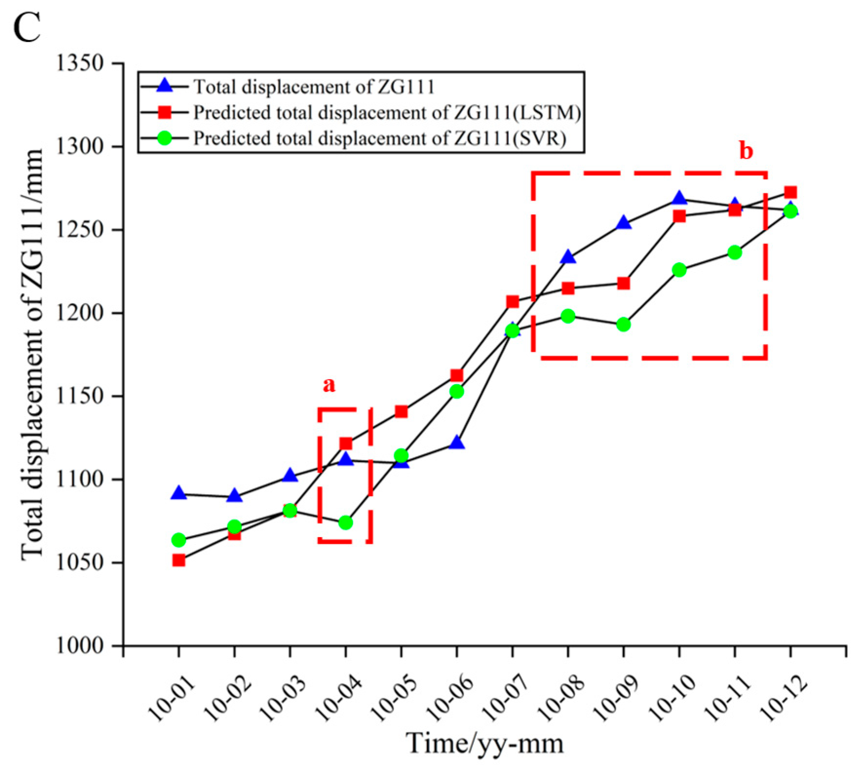
| Time | Original Displacement (mm) | SVRs | LSTMs | ||||
|---|---|---|---|---|---|---|---|
| Predicted Displacement (mm) | Absolute Error (mm) | Relative Error (%) | Predicted Displacement (mm) | Absolute Error (mm) | Relative Error (%) | ||
| January 2010 | 1091.10 | 1063.57 | 27.53 | 2.52 | 1051.56 | 39.54 | 3.62 |
| February 2010 | 1089.50 | 1071.65 | 17.85 | 1.64 | 1067.39 | 22.11 | 2.03 |
| March 2010 | 1101.70 | 1081.30 | 20.4 | 1.85 | 1081.33 | 20.37 | 1.85 |
| April 2010 | 1111.40 | 1074.04 | 37.36 | 3.36 | 1121.60 | 10.20 | 0.92 |
| May 2010 | 1109.80 | 1114.29 | 4.49 | 0.40 | 1140.80 | 31.00 | 2.79 |
| June 2010 | 1121.40 | 1152.87 | 31.47 | 2.81 | 1162.53 | 41.13 | 3.67 |
| July 2010 | 1189.40 | 1189.36 | 0.04 | 0.00 | 1206.89 | 17.49 | 1.47 |
| August 2010 | 1232.90 | 1198.16 | 34.74 | 2.82 | 1214.94 | 17.96 | 1.46 |
| September 2010 | 1253.50 | 1193.15 | 60.35 | 4.81 | 1217.85 | 35.65 | 2.84 |
| October 2010 | 1268.30 | 1225.88 | 42.42 | 3.34 | 1258.32 | 9.98 | 0.79 |
| November 2010 | 1264.20 | 1236.41 | 27.79 | 2.20 | 1261.92 | 2.28 | 0.18 |
| December 2010 | 1262.00 | 1261.16 | 0.84 | 0.07 | 1272.52 | 10.52 | 0.83 |
| Min | 0.04 | 0.00 | 9.98 | 0.18 | |||
| Max | 60.35 | 4.81 | 41.13 | 3.67 | |||
| Mean | 25.44 | 2.15 | 21.52 | 1.87 | |||
| RMSE | 30.71 | 24.73 | |||||
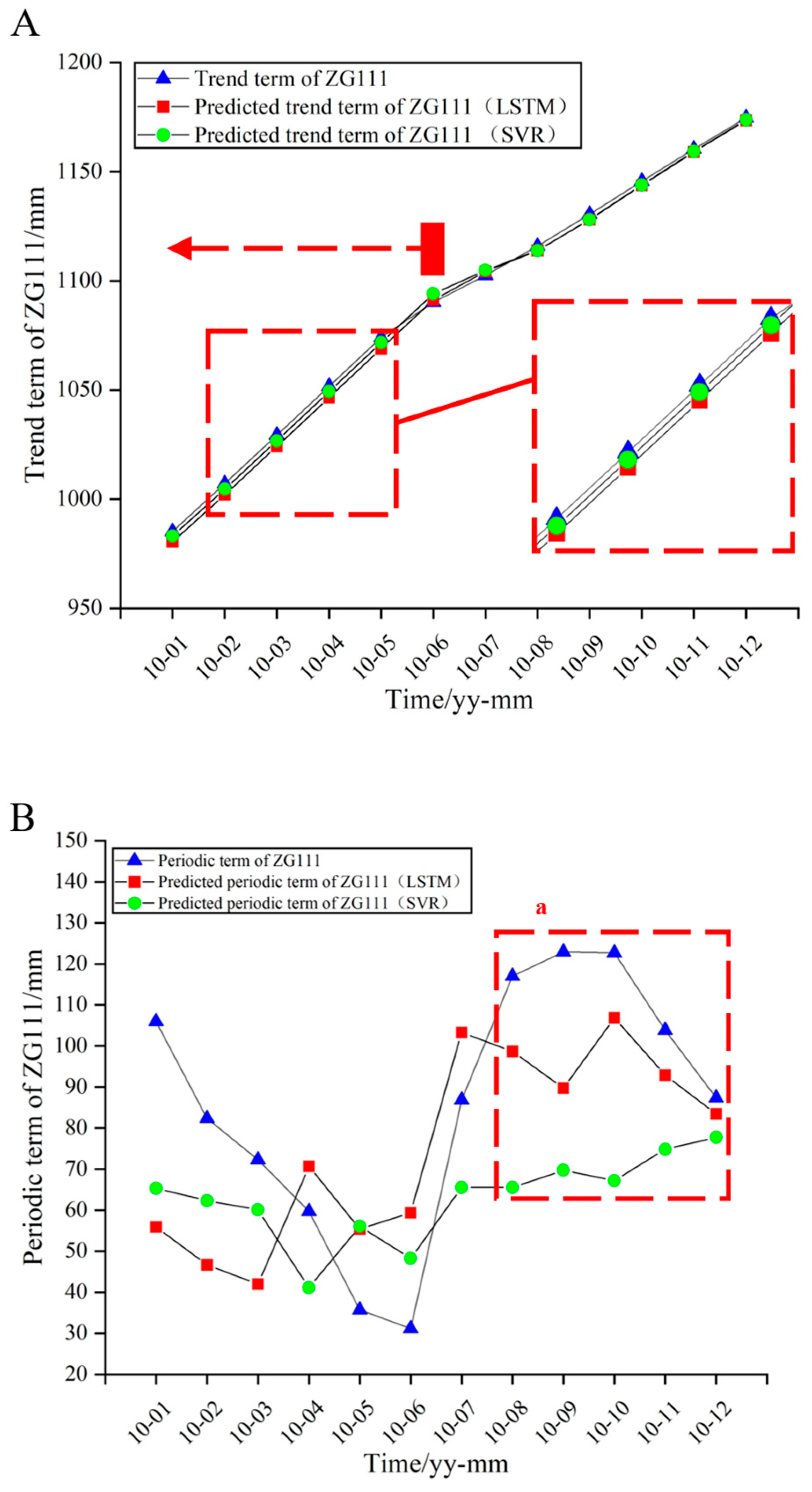
| Model | RMSE in Trend Term (mm) | RMSE in Periodic Term (mm) |
|---|---|---|
| SVR | 2.30 | 28.92 |
| LSTM | 3.52 | 23.61 |
| Inputs | N_NEIGHBORS | P |
|---|---|---|
| f1, f3, f4, f5, f6, f10, f11, f12, f13, f15 | 2 | 2 |
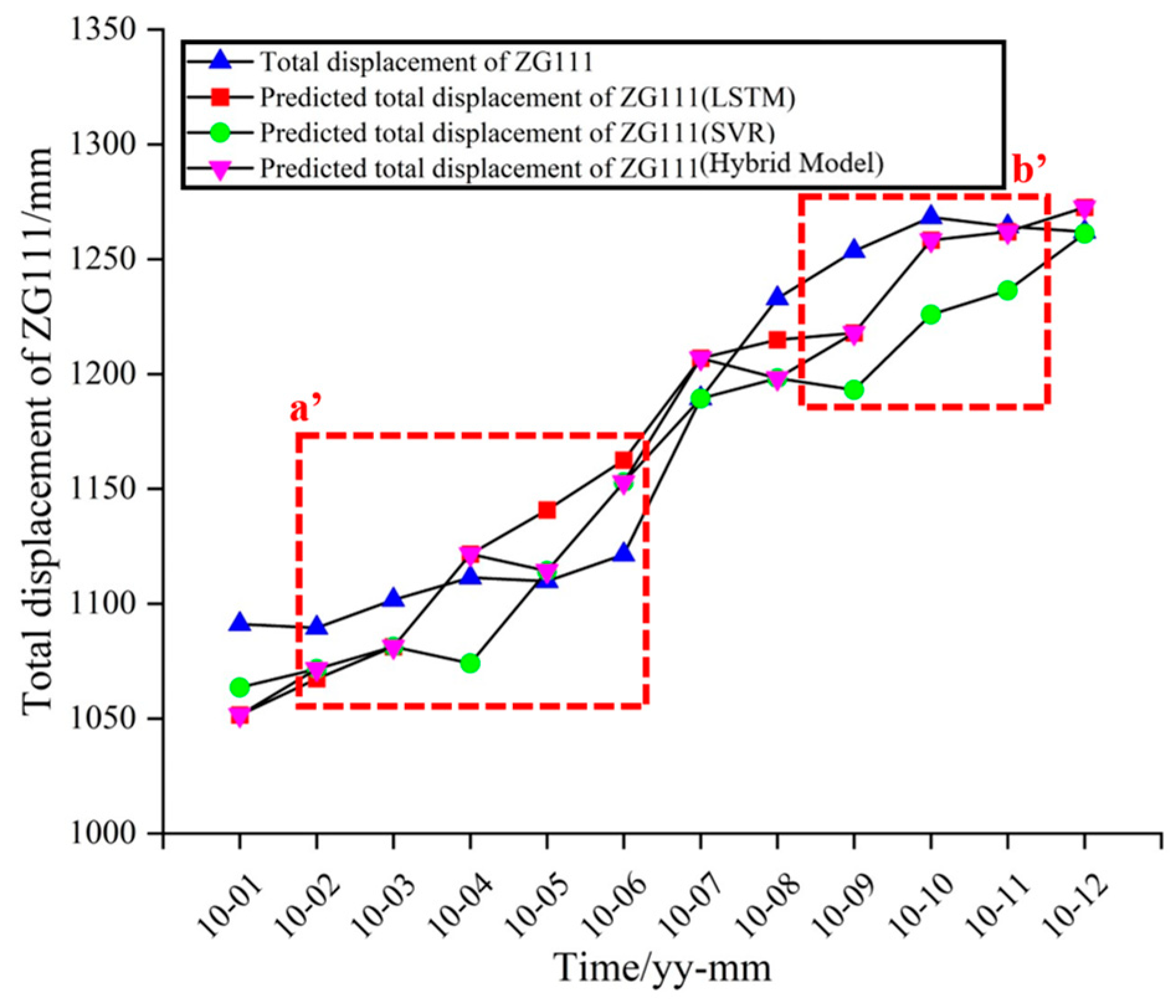
| Time | Original Displacement (mm) | Predicted Displacement (mm) | Classification Output Results | Absolute Error (mm) | Relative Error (%) |
|---|---|---|---|---|---|
| January 2010 | 1091.10 | 1051.56 | 0 | 39.54 | 3.62 |
| February 2010 | 1089.50 | 1071.65 | 1 | 17.85 ^ | 1.64 |
| March 2010 | 1101.70 | 1081.33 | 0 | 20.37 * | 1.85 |
| April 2010 | 1111.40 | 1121.60 | 0 | 10.20 * | 0.92 |
| May 2010 | 1109.80 | 1114.29 | 1 | 4.49 ^ | 0.40 |
| June 2010 | 1121.40 | 1152.87 | 1 | 31.47 ^ | 2.81 |
| July 2010 | 1189.40 | 1206.89 | 0 | 17.49 | 1.47 |
| August 2010 | 1232.90 | 1198.16 | 1 | 34.74 | 2.82 |
| September 2010 | 1253.50 | 1217.85 | 0 | 35.65 * | 2.84 |
| October 2010 | 1268.30 | 1258.32 | 0 | 9.98 * | 0.79 |
| November 2010 | 1264.20 | 1261.92 | 0 | 2.28 * | 0.18 |
| December 2010 | 1262.00 | 1272.52 | 0 | 10.52 | 0.83 |
| Min | 2.28 | 0.18 | |||
| Max | 39.54 | 3.62 | |||
| Mean | 19.55 | 1.68 | |||
| RMSE | 23.11 |
| Point | LSTMs | SVRs | ||||
|---|---|---|---|---|---|---|
| Number of Layers | Number of Epochs | Number of Batch Sizes | Number of Neurons | C | Gamma | |
| Total displacement of ZG111 | 3 | 65 | 28 | 22 | 74.0 | 0.75 |
| Model | RMSE of Single Model in Total Displacement (mm) |
|---|---|
| SVR | 386.93 |
| LSTM | 453.59 |
Disclaimer/Publisher’s Note: The statements, opinions and data contained in all publications are solely those of the individual author(s) and contributor(s) and not of MDPI and/or the editor(s). MDPI and/or the editor(s) disclaim responsibility for any injury to people or property resulting from any ideas, methods, instructions or products referred to in the content. |
© 2025 by the authors. Licensee MDPI, Basel, Switzerland. This article is an open access article distributed under the terms and conditions of the Creative Commons Attribution (CC BY) license (https://creativecommons.org/licenses/by/4.0/).
Share and Cite
Jiang, H.; Wu, J.; Zhou, H.; Liu, M.; Li, S.; Wu, Y.; Guo, Y. The Application of KNN-Optimized Hybrid Models in Landslide Displacement Prediction. Eng 2025, 6, 169. https://doi.org/10.3390/eng6080169
Jiang H, Wu J, Zhou H, Liu M, Li S, Wu Y, Guo Y. The Application of KNN-Optimized Hybrid Models in Landslide Displacement Prediction. Eng. 2025; 6(8):169. https://doi.org/10.3390/eng6080169
Chicago/Turabian StyleJiang, Hongwei, Jiayi Wu, Hao Zhou, Mengjie Liu, Shihao Li, Yuexu Wu, and Yongfan Guo. 2025. "The Application of KNN-Optimized Hybrid Models in Landslide Displacement Prediction" Eng 6, no. 8: 169. https://doi.org/10.3390/eng6080169
APA StyleJiang, H., Wu, J., Zhou, H., Liu, M., Li, S., Wu, Y., & Guo, Y. (2025). The Application of KNN-Optimized Hybrid Models in Landslide Displacement Prediction. Eng, 6(8), 169. https://doi.org/10.3390/eng6080169