Comparative Analysis of Dedicated and Randomized Storage Policies in Warehouse Efficiency Optimization

Abstract

This paper examines the impact of two storage policies—dedicated storage (D-SLAP) and randomized storage (R-SLAP)—on warehouse operational efficiency. It integrates the Storage Location Assignment Problem (SLAP) with the unrelated parallel machine scheduling problem (UPMSP), which represents the scheduling of the material handling equipment (MHE). This integration is intended to elucidate the interplay between storage strategies and scheduling performance. The considered evaluation metrics include transportation cost, average waiting time, and total tardiness, while accounting for product arrival and demand schedules, precedence constraints, and transportation expenses. Additionally, considerations such as MHE eligibility, resource requirements, and available storage locations are incorporated into the analysis. Given the complexity of the combined problem, a tailored Non-dominated Sorting Genetic Algorithm (NSGA-II) was developed to assess the performance of the two storage policies across various randomly generated test instances of differing sizes. Parameter tuning for the NSGA-II was conducted using the Taguchi method to identify optimal settings. Experimental and statistical analyses reveal that, for small-size instances, both policies exhibit comparable performance in terms of transportation cost and total tardiness, with R-SLAP demonstrating superior performance in reducing average waiting time. Conversely, results from large-size instances indicate that D-SLAP surpasses R-SLAP in optimizing waiting time and tardiness objectives, while R-SLAP achieves lower transportation cost.

1. Introduction

Warehouses play a pivotal role in supply chain management by ensuring efficient distribution and balancing supply–demand dynamics. Optimizing storage allocation reduces storage durations, minimizes travel distances, and alleviates product flow bottlenecks, thereby enhancing overall operational efficiency [1]. Furthermore, effective storage coordination streamlines warehouse operations, particularly in order picking tasks. Integrating the processes of storing incoming items and scheduling the material handling equipment (MHE) that are responsible for transporting them to their designated locations is crucial for maximizing resource utilization. Suboptimal location assignments can lead to increased travel distances and congestion, ultimately degrading the MHE scheduling efficiency.

Efficient storage location assignment is critical for warehouse optimization. Recent advancements employ innovative computational techniques to enhance these assignments. Waubert de Puiseau et al. (2022) [2] applied deep reinforcement learning (DRL) to optimize storage locations, demonstrating significant reductions in transportation costs compared to manual methods. However, storage location planning should not be treated in isolation, as it directly impacts order picking efficiency and task scheduling. Bolaños-Zuñiga et al. (2023) [3] developed integrated models that simultaneously optimize storage allocation and picking routes, incorporating product weight to improve operational speed and accuracy. Cai et al. (2021) [4] demonstrated that combining storage planning with robotic path optimization in automated warehouses reduces both time and energy consumption.

A warehouse storage location assignment policy (SLAP) enhances warehouse efficiency by aligning storage capacity with demand, addressing the critical warehousing problem of optimal product allocation. Hausman et al. (1976) [5] pioneered SLAP for automated warehouses, with policies typically classified as dedicated (D-SLAP), class-based, or randomized (R-SLAP) [6]. This study focuses on both dedicated and randomized policies. Traditionally, warehouses relied on D-SLAP, where each product is assigned a fixed storage location. While straightforward, this approach has notable drawbacks, including excessive space requirements to accommodate peak inventory levels for all products [7]. Manzini et al. (2006) [8] showed that D-SLAP in large-scale warehouses leads to significant underutilization of storage space.

In contrast, R-SLAP has gained prominence with advancements in warehouse management systems (WMSs). Bartholdi and Hackman (2008) [9] showed that real-time WMS tracking enables efficient item retrieval, improving space utilization and operational flexibility. Quintanilla et al. (2015) [10] proposed a metaheuristic-based model for R-SLAP optimization, incorporating construction methods and local search algorithms to evaluate relocation strategies. As warehouse complexity increased, advanced optimization techniques emerged. Larco et al. (2017) [11] introduced a mixed-integer linear programming (MILP) framework to minimize order preparation time and worker discomfort, integrating production planning with R-SLAP. Similarly, Tang and Li (2009) [12] applied ant colony optimization (ACO) to optimize product placement, reducing retrieval times and enhancing space efficiency. Zhang et al. (2021) [13] further advanced this field by combining internet of things (IoT)-enabled tracking with randomized storage assignment, improving cost efficiency and space utilization.

The scheduling of MHE operations in a warehouse has the same structure of the parallel machine scheduling problem (PMSP). PMSP involves assigning products to several MHE, such as AGVs or forklifts. The models for the PMSP vary based on the characteristics of the machines involved. In the UPMSP, machines have different speeds and abilities to handle specific tasks [14]. This situation is common in real-world warehouses, where different types of MHE are used for various items. This requires a scheduling approach that considers each task’s requirements, the machines’ capabilities, and their overall performance.

Recent research integrates scheduling and storage allocation assignment to optimize both simultaneously [15]. This approach accounts for interdependencies between scheduling decisions and storage allocations, improving overall efficiency. Applications extend beyond warehousing; for instance, Tang et al. (2016) [16] developed an MILP model for bulk cargo ports, optimizing space allocation and ship scheduling. Fatemi-Anaraki et al. (2021) [17] proposed a mathematical model integrating berth allocation and vessel scheduling in constrained waterways. Chen et al. (2022) [18] introduced an MILP framework combining vehicle routing problems (VRPs) with zone picking, enhancing economic and service performance.

Warehouse operations often involve conflicting objectives, such as minimizing travel time while meeting delivery deadlines. To address this, researchers employed multi-objective optimization approaches. Zhang et al. (2023) [19] optimized storage layouts using a specialized algorithm, balancing picking speed and shelf stability for sustainable operations. Leon et al. (2023) [20] combined simulation and optimization to model real-world conditions, improving storage assignments while considering order picking and routing. Antunes et al. (2022) [21] compared different optimization algorithms and concluded that the choice of a solution approach depends on the problem characteristics. They motivated the choice of NSGA-II for this study.

NSGA-II has proven effective in complex multi-objective engineering optimization problems. Gao et al. (2024) [22] employed NSGA-II to optimize feeder bus route planning, addressing passenger flow, travel time, and cost within a three-dimensional space that included timetable coordination. Their use of NSGA-II demonstrated the algorithm’s capacity to achieve uniform Pareto fronts and adapt to real-time constraints in urban transit systems. Ma et al. (2023) [23] proposed an improved NSGA-II for maritime search and rescue operations under severe weather conditions, emphasizing the algorithm’s ability to balance exploration and exploitation through enhanced population diversity and multi-task knowledge transfer. Niu et al. (2023) [24] utilized NSGA-II for hydrogen production optimization, demonstrating its robustness under fluctuating power inputs. These recent studies underscore NSGA-II’s adaptability, supporting its adoption in this study for optimizing warehouse operations.

Despite extensive research on warehouse optimization, few studies address the joint optimization of storage location assignment (SLAP) and MHE scheduling decisions. This work bridges this critical gap by conducting a comparative analysis of two fundamental storage policies—Dedicated (D-SLAP) and Randomized (R-SLAP)—while simultaneously optimizing transportation costs, waiting times, and order lateness in warehouse operations.

This research is motivated by the growing operational complexity of modern warehouses, where co-optimization of storage allocation and MHE scheduling is essential for maximizing efficiency. By integrating SLAP with UPMSP, we present a multi-objective framework to evaluate how these policies differentially impact warehouse performance metrics, including cost efficiency and customer satisfaction.

Both SLAP and UPMSP are NP-hard combinatorial problems, rendering exact optimization methods computationally intractable. To address this, we leverage NSGA-II, a metaheuristic tailored for multi-objective optimization under conflicting criteria. NSGA-II is selected due to its:

• Proven efficacy in Pareto front exploration, ensuring balanced trade-offs between objectives (e.g., minimizing transportation costs vs. tardiness).
• Adaptability to problem-specific constraints, achieved through a customized three-string chromosome encoding that jointly optimizes scheduling and storage decisions.
• Established robustness in logistics literature.

The proposed framework is validated via rigorous computational benchmarking and statistical testing, comparing D-SLAP and R-SLAP across scalable problem instances. Accordingly, the key contributions of this study are as follows:

• Novel Integration of SLAP and UPMSP: A unified optimization model incorporating real-world constraints (precedence relationships, machine eligibility, limited resources, and dynamic product flows).
• Algorithmic Innovation: A modified NSGA-II with a three-string chromosome representation, enabling simultaneous optimization of storage allocation and MHE scheduling.
• Policy-Centric Benchmarking: A data-driven evaluation of D-SLAP and R-SLAP using multi-objective performance metrics (hypervolume, spacing) and parametric and nonparametric statistical tests, providing actionable insights for warehouse design.

The paper is structured as follows: Section 2 formulates the problem and details the proposed NSGA-II implementation, including performance metrics and parameter tuning. Section 3 presents experimental results across generated test instances. Section 4 provides statistical analysis of the findings. Section 5 concludes with key insights and future research directions.

2. Materials and Methods

This research proposes a comparative study of the performance of D-SLAP and R-SLP while utilizing an integrated strategy for scheduling MHE and storing goods in warehouses.

2.1. Problem Definition

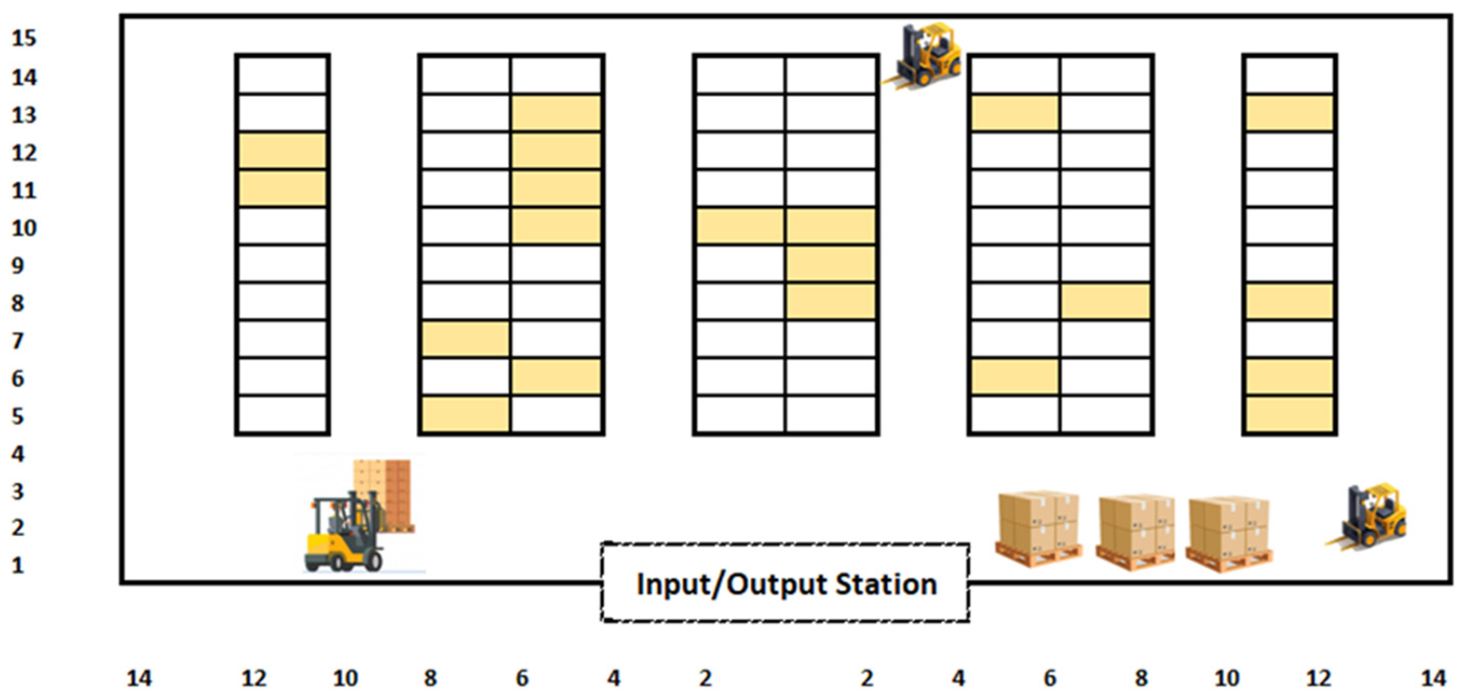
The products are transported from the input/output (I/O) station to the assigned storage locations in the warehouse. Both dedicated and randomized storage policy is applied for SLAP. As shown in Figure 1, the warehouse layout is designed with wide aisles to ensure safe and efficient operation. To maximize storage capacity, vertical space is utilized with two storage levels available at each location. The I/O station, located in the center of the warehouse, serves both incoming and outgoing items. Each item represents a category of products, referred to as jobs. The warehouse is arranged into numbered locations for storage, with each location capable of holding a single pallet at a time. The total number of these locations is known in advance.

Various MHE, such as forklifts, trucks, and automated guided vehicles (AGVs), transport goods. All MHE are available at the start of the scheduling process and can access any storage location. However, they can only handle one job when moving a product to a storage location. No preemption or interruption is allowed during job processing. Products can only be handled when the needed and eligible machine and other required resources are available. Every product is moved and stored as pallets. These pallets vary in size, weight, and geometric configuration, hence the eligibility of specific machines to handle certain jobs. Due to the stacking of pallets above, beside, and in front of one another, precedence constraints exist between some jobs. In addition, a job can only be moved to a storage location if that location is unoccupied. This ensures that no overlap occurs with jobs stored previously in the exact location. Transportation times between the I/O station and storage locations depend on the machine and the location. On the other hand, processing times, which represent loading and unloading, are job- and MHE-dependent.

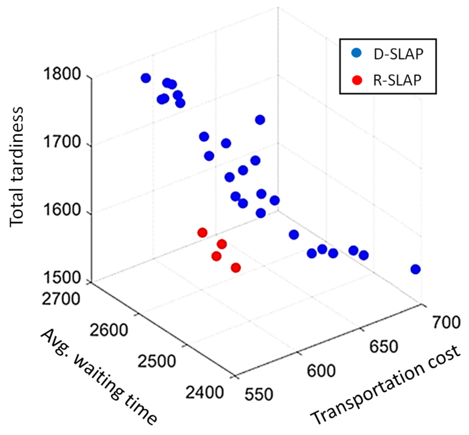
The key objective is to determine the optimal timing for moving products using the appropriate MHE and assigning storage locations, while minimizing transportation costs, waiting times, and lateness. Based on both D-SLAP and R-SLAP, three objectives need to be considered. The first objective (${OF}_1$) corresponds to the cost of transporting products using the appropriate MHE for the designated storage locations. The second objective (${OF}_2$) accounts for the waiting time of products at the I/O station before transferring them to their designated storage locations. The third objective (${OF}_3$) is the total tardiness in meeting the required due dates.

This research proposes a novel integrated optimization framework for simultaneous MHE scheduling and storage location assignment. Given the NP-hard complexity inherent to these combinatorial problems [25], traditional exact solution methods become computationally intractable for practical-scale instances. To overcome this computational limitation, a customized NSGA-II implementation is proposed in this study, specifically designed for this integrated optimization challenge. The metaheuristic approach provides an efficient Pareto solution frontier while maintaining computational feasibility.

2.2. Non-Dominated Sorting Genetic Algorithm (NSGA-II)

NSGA-II is a widely adopted metaheuristic for solving multi-objective optimization problems [26,27]. Developed by Deb et al. (2002) [28], NSGA-II employs a genetic algorithm framework to identify Pareto-optimal solutions through mechanisms such as selection, crossover, mutation, and Pareto-based ranking.

The algorithm begins by generating an initial population of feasible solutions randomly. This population evolves over iterations by applying different genetic operations such as selecting parents, crossover, mutation, and ranking solutions into non-dominated fronts. In the proposed technique, each solution (chromosome) is encoded using three distinct strings: (1) a job sequence, (2) a machine assignment, and (3) a location assignment. The length of each string corresponds to the number of jobs (N) to be scheduled. To ensure compliance with precedence constraints, a corrective algorithm proposed by Afzalirad et al. (2016) [14] is used to adjust the job order and make it feasible. The machine assignment string is generated by randomly assigning an eligible machine to each job. The location assignment string varies depending on the storage policy.

• Under D-SLAP, each job is assigned a dedicated storage location, ensuring that items do not share storage spaces.
• Under R-SLAP, jobs are allocated to any available storage location at random.

An expanded double-point crossover operator is employed to explore neighborhood solutions. Using tournament selection, two parent chromosomes (Pr₁ and Pr₂) are selected. Two crossover points are randomly selected from a discrete uniform distribution, and gene segments between these points are exchanged to produce offspring (Ch₁ and Ch₂). The remaining positions in each child are filled with unassigned genes from the respective parent while preserving their original order.

To ensure feasibility, a corrective mechanism is applied to the job sequence strings. For the machine assignment strings, a random number (r ∈ [0,1]) is generated for each gene. If r > 0.5, the machine assignment is inherited from the opposite parent; otherwise, it is retained from the same parent. The location assignment follows a similar approach: if r > 0.5, the location is inherited from the parent; otherwise, a random feasible location is assigned. Post-crossover, a repair mechanism may be applied to maintain the feasibility of the generated solution.

A mutation operator enhances population diversity. A chromosome is randomly selected, and two genes in its job sequence string are swapped. If the resulting sequence violates precedence constraints, the correction mechanism is applied. For the machine assignment string, unchanged genes retain their parent assignments, while swapped genes undergo reassignment: if a number is randomly generated (r < 0.5), the original machine is retained; otherwise, a new eligible machine is selected. The location assignment string is generated based on the storage policy. For D-SLAP, each job is assigned a random dedicated storage location, while for R-SLAP, each job is assigned a random available storage location.

NSGA-II employs non-dominated sorting to classify solutions into Pareto fronts based on dominance relationships. Solutions within each front are further ranked using crowding distance, a measure of solution density in the objective space, to promote diversity. The algorithm terminates after a predefined number of iterations, yielding a set of non-dominated solutions.

2.3. Performance Metrics

Several metrics are used to evaluate the performance of multi-objective optimization algorithms [29]. In this study, the used metrics are the number of solutions in the Pareto front (NPS), the Mean Ideal Distance (MID), a metric for diversification (DM), and a metric that evaluates the solutions’ dispersion (SNS). Finally, a Quality Metric (QM) that compares the dominance of solutions and calculates the percentage of solutions that belong to each storage policy is used. Equations (1) to (3) explain how these metrics are evaluated. In these equations, the index $i$ refers to a Pareto front solution, while ${OF}_j$ is the jth objective function value.

$$DM=\sqrt{\sum _{j=1}^3{(\underset{i}{\max }\left({\mathit{OF}}_{j,i}\right)-\underset{i}{\min }\left({OF}_{j,i}\right))}^2}$$

(1)

$$MID={\displaystyle \frac{\sum _{i=1}^{NPS}{c}_i}{NPS}}$$

(2)

where $c_i=\sqrt{\sum _{j=1}^3{{OF}_{j,i}}^2}$.

$$SNS=\sqrt{{\displaystyle \frac{\sum _{i=1}^{NPS}{(MID-c}_i)}{NPS-1}}}$$

(3)

2.4. Parameter Tuning

Metaheuristic algorithms require careful parameter selection to ensure optimal performance. In this study, the Taguchi method is employed to determine the best parameter combinations for the NSGA-II algorithm. This approach efficiently evaluates multiple decision variables with fewer experiments by leveraging orthogonal arrays (OAs) instead of full factorial designs [30].

For the proposed NSGA-II implementation, the following parameters are optimized: maximum number of iterations, population size, crossover rate, and mutation rate. An L9 OA is utilized to test each parameter at three distinct levels, as outlined in

Table 1. Parameter tuning of NSGA-II.

Parameters	Level
	1	2	3
Maximum iterations	200	350	500
Population size	50	75	100
Crossover rate	0.6	0.75	0.9
Mutation rate	0.01	0.05	0.1

. These levels are selected to accommodate both small and large test instances under D-SLAP and R-SLAP scenarios.

The NSGA-II algorithm is executed across all parameter combinations of the L9 OA, with each configuration evaluated over 10 replications. To assess performance, two key metrics are employed: Relative Percentage Deviation (RPD) and the signal-to-noise (S/N) ratio. The RPD, calculated using Equation (4), normalizes the acquired results. Here, the solution is the value of the performance measure acquired by each test instance, and Best is the best value of the performance measure obtained over all replications of this instance. The RPD provides a measure of the algorithms’ relative performance.

$$\mathrm{R}\mathrm{P}\mathrm{D}={\displaystyle \frac{{|\mathrm{P}\mathrm{o}\mathrm{l}\mathrm{i}\mathrm{c}\mathrm{y}}_{\mathrm{s}\mathrm{o}\mathrm{l}}-{\mathrm{B}\mathrm{e}\mathrm{s}\mathrm{t}}_{\mathrm{s}\mathrm{o}\mathrm{l}}|}{{\mathrm{B}\mathrm{e}\mathrm{s}\mathrm{t}}_{\mathrm{s}\mathrm{o}\mathrm{l}}}}\times 100$$

(4)

The Taguchi method only deals with one response variable. Therefore, the weighted mean of the performance measures (WMPM) is identified as in Equation (5).

$$\mathrm{W}\mathrm{M}\mathrm{P}\mathrm{M}={\displaystyle \frac{\mathrm{N}\mathrm{P}\mathrm{S}+\mathrm{D}\mathrm{M}+2\ast \mathrm{M}\mathrm{I}\mathrm{D}+\mathrm{S}\mathrm{N}\mathrm{S}+2\ast \mathrm{Q}\mathrm{M}}{7}}$$

(5)

In addition, the average value for 10 replications is calculated. The signal-to-noise (S/N) ratio is used to reduce the variation in the response variable. According to the Taguchi method, the S/N ratio for minimizing objectives is calculated using Equation (6).

$$\mathrm{S}/\mathrm{N}=-10\times {\mathrm{l}\mathrm{o}\mathrm{g}}_{10}{\left(\mathrm{o}\mathrm{b}\mathrm{j}\mathrm{e}\mathrm{c}\mathrm{t}\mathrm{i}\mathrm{v}\mathrm{e}\mathrm{f}\mathrm{u}\mathrm{n}\mathrm{c}\mathrm{t}\mathrm{i}\mathrm{o}\mathrm{n}\right)}^2$$

(6)

The best parameter combinations for small- and large-sized instances are summarized in

Table 2. Best parameter settings of NSGA-II.

Parameter	NSGA-II
	Best Level	Level Value
Maximum iterations	2	350
Population size	3	200
Crossover rate	2	0.75
Mutation rate	3	0.1

. For each parameter of the NSGA-II algorithm, its best value is indicated as it provides a minimum value of WMPM and a maximum value of the S/N ratio. Figure 2 and Figure 3 display the average WMPM and signal-to-noise (S/N) ratio obtained for the NSGA-II algorithm at the different levels of the studied parameters, respectively. Accordingly, Table 2 summarizes the best parameter combinations for the problem using D-SLAP and R-SLAP based on these figures.

3. Results

The computational experiments were conducted on a workstation equipped with an 11th-generation Intel^® Core^TM i9-11900K processor and 32 GB of RAM. The proposed NSGA-II was implemented in MATLAB R2020a and evaluated on 24 test instances, evenly split between 12 small-size and 12 large-size cases. Each instance was solved under both D-SLAP and R-SLAP policies to compare their performance.

3.1. Experimental Design

To compare the performance of the D-SLAP and R-SLAP policies under the proposed efficient multi-objective optimization NSGA-II metaheuristic for the integration of UPMSP and SLAP, the 24 test instances were designed by varying five key problem parameters: the number of items, machines, jobs, storage locations, and resource availability. Temporal parameters were generated using discrete uniform distributions. For small-size instances, processing times were sampled from U(1,10), while large-size instances used U(1,20). Setup times followed U(1,4) minutes for small instances and U(3,6) minutes for large instances. Release dates were assigned within U(1,30) for small instances and U(1,50) for large instances. The due date $D_j$ for each job $j$ was calculated using Equation (7), where $R_j$ represents its release time, U(2,5) × 10 generates a random integer multiple of 10 between 20 and 50, and $max \left(P_{jm}\right)$ denotes the maximum processing time of job $j$ across all MHE.

$$D_j=R_j+U\left(2,5\right)\times 10+max \left(P_{jm}\right)$$

(7)

The problem constraints were implemented through two binary matrices. A precedence matrix encoded job sequencing dependencies, while an MHE eligibility matrix ensured that each job could be processed by at least half of the available MHE (rounded down), following the methodology established in [14].

Cost parameters were uniformly distributed, with transportation and processing costs $C_j$ ranging between 1 and 10 for all instances. All jobs associated with the same item were assigned identical transportation costs and processing times when executed by the same MHE. MHE speeds differed by instance size: small instances used speeds between 5 and 8 km/h (U(5,8)), while large instances employed faster MHE at 8–10 km/h (U(8,10)). Transportation times were computed based on rectilinear (Manhattan) distances between the I/O station at (0,0,0) and storage locations at (x,y,z), where z remained fixed per rack level. The distance calculation between coordinates $(x_1,y_1)$ and $(x_2,y_2)$ followed $\left|x_2-x_1\right|+\left|y_2-y_1\right|$, as established in [31] for grid-based warehouse environments. This approach provides an accurate representation of real-world travel paths in warehouse settings.

3.2. NSGA-II Performance Under D-SLAP and R-SLAP

Table 3. Comparison of performance metrics of NSGA-II with respect to storage policies for small-sized test instances.

No.	I	N	M	L	R	NPS		DM		MID		SNS		QM
						D-SLAP	R-SLAP	D-SLAP	R-SLAP	D-SLAP	R-SLAP	D-SLAP	R-SLAP	D-SLAP	R-SLAP
1	2	4	2	2	1	100	100	14.42	14.42	174.44	174.85	1.5978	1.39	50	50
2	2	4	2	2	2	100	100	0	0	163.39	149.34	0	0	50	50
3	3	4	3	4	1	100	100	10.38	34.69	51.38	49.86	2.77	3.85	50	50
4	3	4	3	4	2	100	100	9.28	42.3	55.35	54.13	1.01	6.4	50	50
5	2	6	2	2	1	100	100	0	0	262.61	262.61	0	0	50	50
6	2	6	2	2	2	100	100	33.35	35.06	178.98	181.72	5.27	3.67	50	50
7	3	6	3	4	1	100	100	21.55	54.40	158.27	112.12	3.23	4.34	50	50
8	3	6	3	4	2	100	100	156.70	39.55	162.35	134.8	48.95	5.57	50	50
9	2	8	2	4	1	100	100	197.36	69.79	369.75	352.59	58.9	13.01	50	50
10	2	8	2	4	2	100	100	101.14	87.44	313.43	307.18	14.71	13.15	50	50
11	3	8	3	6	1	100	100	200.09	160.69	473.69	470.74	27.34	20.33	50	50
12	3	8	3	6	2	100	100	29.29	35.536	384.30	382.68	3.08	2.62	50	50
Average value						100	100	64.46	47.82	229	219.39	13.91	6.194	50	50

A bold value indicates the optimal storage policy for each metric.

presents a comparative analysis of the algorithm’s performance under D-SLAP and R-SLAP for small-size test instances, evaluated across the five key performance metrics. Both algorithms consistently achieved 100 solutions in the Pareto front, indicating comparable solution quality and optimality. However, D-SLAP exhibited a more uniform distribution of solutions along the Pareto front compared to R-SLAP, suggesting better diversity in its solution set. Conversely, R-SLAP generated solutions with smaller metric values, implying closer proximity to the ideal point and thus higher solution quality in certain aspects.

Table 4. Comparison of performance metrics of NSGA-II with respect to storage policies for large-sized test instances.

No.	I	N	M	L	R	NPS		DM		MID		SNS		QM
						D-SLAP	R-SLAP	D-SLAP	R-SLAP	D-SLAP	R-SLAP	D-SLAP	R-SLAP	D-SLAP	R-SLAP
1	3	20	4	10	2	85.1	100	1258.8	699.8	1890.2	1956	330.9	148	18.81	81.18
2	3	30	4	10	3	76	100	2095.9	727.5	3230.8	3189.2	509.4	77	9.78	90.22
3	3	40	6	20	4	76.2	100	2712.5	729.7	5284.2	5012.3	611.2	178.3	4.13	95.88
4	3	50	6	20	5	72.1	100	6543.8	1423.9	11,118.8	9680.6	15,395	246.6	4.42	95.58
5	4	20	4	10	2	60.7	100	691.5	235.2	2085.6	2093.3	124.3	30.8	2.79	97.20
6	4	30	4	10	3	85.1	100	1286.6	729.1	3362.3	3303	294.3	93.8	13.83	86.17
7	4	40	6	20	4	73.3	100	3146.9	949.6	6638.09	6827.5	639.3	192.7	9.44	90.56
8	4	50	6	20	5	78.2	100	4847.9	811.6	9704.12	9105.1	983.8	231.9	3.82	96.19
9	5	20	4	10	2	95	100	1080.2	505.4	1657.65	1721.3	231.2	67.7	29.11	70.9
10	5	30	4	10	3	94.8	99.8	2142.5	1043.5	3277.47	3383.9	394.7	159.9	23.78	76.23
11	5	40	6	20	4	64.7	98	2700.7	1327.5	6497.6	6620.5	591.9	291.4	9.88	90.12
12	5	50	6	20	5	80.8	100	5690.6	1088.1	9759	9840.4	1118.7	172	9.95	90.05
Average value						78.5	99.8	2849.8	855.9	5375.5	5227.8	1768.7	157.51	11.65	88.36

A bold value indicates the optimal storage policy for each metric.

presents a comparative evaluation of D-SLAP and R-SLAP for large-size instances. The results indicate that R-SLAP achieves superior performance in terms of SNS, MID, and QM, demonstrating its effectiveness in identifying efficient Pareto front solutions across all configurations. Furthermore, R-SLAP generates solutions that are consistently closer to the ideal point. In contrast, D-SLAP exhibits better performance in SNS and DM, indicating a more uniform distribution of solutions along the Pareto front.

Figure 4 illustrates a comparative analysis of the performance of NSGA-II under D-SLAP and R-SLAP policies across three objectives for the fifth replication of the second large-sized test instance. The solutions obtained by D-SLAP are widely dispersed across the solution space, reflecting the differences between the ARPD values of D-DLAP and R-SLAP are calculated for each instance greater diversity and a balanced trade-off among objectives. Conversely, R-SLAP’s solutions are concentrated within a narrower region, resulting in reduced solution variety compared to D-SLAP.

3.3. D-SLAP Versus R-SLAP Comparative Results

The comparison of D-SLAP versus R-SLAP is conducted across the three objective functions, with the results averaged over ten replications. For small test instances (

Table 5. Comparison of objective functions’ average values of storage policies for small-sized test instances.

No.	I	N	M	L	R	Transportation Cost		Average Waiting Time		Total Tardiness
						D-SLAP	R-SLAP	D-SLAP	R-SLAP	D-SLAP	R-SLAP
1	2	4	2	2	1	150	150	71	71	46	46
2	2	4	2	2	2	92	92	128	114	43	29
3	3	4	3	4	1	38	43.8	31.1	15.5	0	0
4	3	4	3	4	2	44	44	33.1	14.5	0	0
5	2	6	2	2	1	114	114	212	212	105	105
6	2	6	2	2	2	40	40	176	156.1	28	47.2
7	3	6	3	4	1	94.7	86.1	110.5	54.6	42.4	8.6
8	3	6	3	4	2	59.8	56.5	96.9	105.3	4.1	13.3
9	2	8	2	4	1	66	80.6	320	307.1	129	110.4
10	2	8	2	4	2	152	152	254.2	223	82.6	65.4
11	3	8	3	6	1	336	336	234.2	240.8	56.5	62.4
12	3	8	3	6	2	300.3	300.3	224.4	226	69.1	71.6

A bold value indicates the optimal storage policy for each objective.

), both policies perform comparably in the total tardiness, while R-SLAP outperforms D-SLAP in the average waiting time for most cases; the transportation cost shows marginal differences, with each policy excelling in select instances. This suggests R-SLAP’s superiority for the average waiting time and highlights the flexibility of randomized storage in small systems due to unconstrained slot allocation. For large instances (

Table 6. Comparison of objective functions’ average values of storage policies for large-sized test instances.

No.	I	N	M	L	R	Transportation Cost		Average Waiting Time		Total Tardiness
						D-SLAP	R-SLAP	D-SLAP	R-SLAP	D-SLAP	R-SLAP
1	3	20	4	10	2	302.2	294.8	1331.1	1392.3	871.6	930.7
2	3	30	4	10	3	630.6	581	2258.2	2477.2	1411.4	1582
3	3	40	6	20	4	1188	1056.9	3687.3	3690.9	2595.6	2551.3
4	3	50	6	20	5	1257.3	983.1	7251.3	7100.2	6122.8	5881.7
5	4	20	4	10	2	404.8	396.2	1648.4	1675.2	1107	1131.8
6	4	30	4	10	3	696.9	676	2449.8	2493.1	1620	1646.2
7	4	40	6	20	4	1033	851	4792.5	5039.8	3723	3935.9
8	4	50	6	20	5	1096.9	900.5	6793.3	6883.5	5415.6	5466.9
9	5	20	4	10	2	554.9	515.3	1118.1	1257.9	698.2	848.2
10	5	30	4	10	3	710.5	643.1	2447.7	2654.5	1663.5	1834.3
11	5	40	6	20	4	1395.4	1117.4	4713.3	4808.3	3595.3	3653.3
12	5	50	6	20	5	2255.9	1921.9	6755.1	7247.8	5238.5	5719

A bold value indicates the optimal storage policy for each objective.

), R-SLAP dominates the transportation cost objective, achieving superior results in 11 out of 12 cases, whereas D-SLAP excels in average waiting time and total tardiness for most instances, despite R-SLAP’s competitiveness in sporadic cases. Collectively, these findings demonstrate that R-SLAP is preferable for the transportation cost regardless of system scale, while D-SLAP proves more effective for the other objectives in large-scale configurations.

To compare the performance of the two SLAP policies with respect to each individual objective, the Relative Percentage Deviation (RPD) is evaluated. The RPD is calculated for each instance based on the best solution obtained among the two storage policies, as provided in Equation (8).

$$\mathrm{R}\mathrm{P}\mathrm{D}={\displaystyle \frac{{|\mathrm{B}\mathrm{e}\mathrm{s}\mathrm{t}}_{\mathrm{F}\mathrm{r}\mathrm{o}\mathrm{n}\mathrm{t}}-{\mathrm{B}\mathrm{e}\mathrm{s}\mathrm{t}}_{\mathrm{s}\mathrm{o}\mathrm{l}}|}{{\mathrm{B}\mathrm{e}\mathrm{s}\mathrm{t}}_{\mathrm{s}\mathrm{o}\mathrm{l}}}}\times 100$$

(8)

To provide a visual comparison of the two policies using the RPD, interval plots at 95% confidence level are drawn for each objective individually. For small-size instances (Figure 5, Figure 6 and Figure 7), the interval plots reveal distinct performance patterns across the three objectives. For the transportation cost objective (Figure 5), D-SLAP demonstrates a mean RPD value of 8.5 compared to R-SLAP’s 10.0, with partial confidence interval (CI) overlap suggesting potential statistical equivalence, though D-SLAP’s marginally lower RPD may indicate slight superiority. For the average waiting time, Figure 6 shows a pronounced performance difference, with D-SLAP’s mean RPD of 40.0 substantially exceeding R-SLAP’s 5.0; the complete confidence interval separation confirms statistical significance, establishing R-SLAP’s clear advantage. For total tardiness (Figure 7), D-SLAP’s mean RPD (75.0) is less than half of R-SLAP’s (175.0), yet overlapping CIs suggest that this difference may not be statistically significant. The aggregate analysis indicates comparable performance between policies for the transportation cost and the total tardiness, but R-SLAP’s decisive superiority in the average waiting time.

The large instance analysis reveals statistically significant performance divergences across all objectives. Regarding the transportation cost (Figure 8), R-SLAP achieves a markedly lower mean RPD (5.5 versus D-SLAP’s 20.0), with non-overlapping CIs con-firming its statistical superiority. This trend reverses for the average waiting time (Figure 9), where D-SLAP’s mean RPD (7.5) significantly outperforms R-SLAP’s 12.5, as evidenced by distinct CIs. The pattern continues in the total tardiness (Figure 10), with D-SLAP maintaining superiority (mean RPD 12.5 vs. R-SLAP’s 18.5) and non-overlapping CIs validating the statistical significance of this advantage. These results demonstrate a consistent performance inversion between instance sizes: while R-SLAP dominates the transportation cost regardless of scale, D-SLAP shows increasing superiority for the other two objectives as instance size grows.

3.4. Demonstrative Example Using Data of Large Instance 1

As a demonstrative example, this section provides the detailed values of the parameters for the first large-size test instance, as given in

Table 7. Input parameters of demonstrative example.

Job	Item	RT	DT	RR	Cost	Direct Successors	Processing Time
							M1	M2	M3	M4
1	2	3	33	2	4	2, 3, 4, 5, 8, 9, 11, 14, 15, 17, 20	1	7	10	8
2	2	33	93	2	4	5, 6, 8, 9, 13, 15, 17, 18	1	7	10	8
3	1	3	33	2	4	4, 6, 7, 8, 10, 12, 16, 17, 18, 19, 20	6	6	1	4
4	2	48	98	2	4	7, 13,14, 18, 19	1	7	10	8
5	3	34	84	2	2	7, 8, 10, 11, 14, 16, 17, 18, 19, 20	2	5	7	7
6	3	21	61	2	2	7, 9, 13, 15, 16, 19	2	5	7	7
7	1	43	83	2	4	10, 13, 15, 17, 19	6	6	1	4
8	2	27	77	2	4	10, 13, 14, 15, 18, 19, 20	1	7	10	8
9	2	8	48	2	4	12, 14, 15, 16, 17	1	7	10	8
10	1	24	74	2	4	11, 12, 13, 16, 17, 18	6	6	1	4
11	2	26	66	2	4	12, 13, 15, 17, 18	1	7	10	8
12	3	17	57	2	2	14, 16, 17, 19, 20	2	5	7	7
13	3	1	31	2	2	16, 17, 18, 20	2	5	7	7
14	3	47	87	2	2	16, 18, 19, 20	2	5	7	7
15	3	1	51	2	2		2	5	7	7
16	2	21	61	2	4	17, 20	1	7	10	8
17	2	47	107	2	4	19, 20	1	7	10	8
18	1	31	91	2	4		6	6	1	4
19	1	24	54	2	4	20	6	6	1	4
20	1	50	110	2	4		6	6	1	4

RT, DT, RR, M: Ready Time (T); due date (DT); required resources (RR); machine (M).

,

Table 8. Travel times of demonstrative example.

MHE/Location	L1	L2	L3	L4	L5	L6	L7	L8	L9	L10
M1	4	4	5	5	6	4	4	5	5	6
M2	5	5	6	6	8	5	5	6	6	8
M3	4	4	5	5	6	4	4	5	5	6
M4	4	4	6	6	7	4	4	6	6	7

,

Table 9. Eligibility constraints of demonstrative example.

MHE/Job	1	2	3	4	5	6	7	8	9	10	11	12	13	14	15	16	17	18	19	20
1	0	0	1	0	1	1	1	0	0	1	0	1	1	1	1	0	0	1	1	1
2	1	1	1	1	1	1	1	1	1	1	1	1	1	1	1	1	1	1	1	1
3	0	0	0	0	1	1	0	0	0	0	0	1	1	1	1	0	0	0	0	0
4	1	1	1	1	0	0	1	1	1	1	1	0	0	0	0	1	1	1	1	1

,

Table 10. The setup times of the demonstrative example on MHE 1.

From/to	1	2	3	4	5	6	7	8	9	10	11	12	13	14	15	16	17	18	19	20
0	4	4	5	3	5	4	4	5	3	6	3	3	6	4	6	5	4	4	5	4
1	0	4	4	4	3	5	3	3	6	3	4	3	5	5	6	6	4	3	4	4
2	5	0	4	5	3	4	6	3	3	3	5	5	5	6	3	3	6	3	6	4
3	4	4	0	5	4	3	3	3	4	4	5	4	3	5	5	3	4	4	4	5
4	6	4	5	0	4	3	6	5	4	5	4	6	3	3	3	5	6	5	5	5
5	4	4	3	5	0	6	5	3	5	5	6	3	5	6	3	6	3	5	5	3
6	5	5	6	6	4	0	5	6	6	4	3	6	5	3	3	6	5	3	5	3
7	6	3	6	5	3	4	0	6	3	6	4	3	5	6	3	3	5	6	5	4
8	4	4	6	4	5	3	5	0	5	6	3	3	6	6	3	3	5	5	6	4
9	6	6	6	6	6	3	6	5	0	5	5	4	5	4	5	3	3	4	5	3
10	4	4	4	6	4	4	4	5	6	0	6	6	6	6	4	4	5	3	3	4
11	4	5	4	4	5	6	3	5	5	5	0	3	5	6	6	5	3	4	6	4
12	6	6	6	5	6	3	5	3	3	3	4	0	3	3	5	5	6	4	5	4
13	4	5	4	4	6	6	6	5	6	3	3	4	0	5	6	5	6	6	3	3
14	3	5	5	5	4	5	5	5	5	6	3	6	6	0	5	5	6	3	5	3
15	3	3	4	6	4	5	6	4	6	5	5	6	3	3	0	5	6	3	3	6
16	3	3	5	6	3	6	3	5	4	6	5	3	6	4	3	0	5	3	3	4
17	6	3	5	6	3	6	6	5	3	5	6	5	4	5	3	4	0	6	6	3
18	5	3	4	6	5	6	3	3	4	5	6	4	4	6	4	4	5	0	4	4
19	3	5	5	6	3	3	4	4	3	3	6	6	5	6	6	6	4	5	0	4
20	4	4	5	6	5	3	5	6	3	6	6	6	4	4	4	3	3	4	3	0

,

Table 11. The setup times of the demonstrative example on MHE 2.

From/to	1	2	3	4	5	6	7	8	9	10	11	12	13	14	15	16	17	18	19	20
0	3	3	3	4	4	4	4	4	3	3	4	5	4	5	4	5	6	6	6	5
1	0	5	3	4	4	3	6	5	3	5	5	4	6	4	6	6	6	4	4	4
2	5	0	5	4	6	5	3	3	5	6	4	3	4	3	3	5	3	6	6	5
3	6	6	0	5	3	5	6	4	4	4	5	4	3	3	3	3	6	3	5	6
4	5	3	4	0	3	4	4	6	4	4	5	6	4	4	3	4	6	6	6	3
5	5	3	4	5	0	4	3	5	6	3	3	4	3	3	6	3	5	6	6	4
6	4	3	6	3	4	0	5	3	4	3	5	6	3	4	3	5	5	3	6	4
7	6	6	3	4	3	4	0	5	5	6	5	4	3	4	6	3	5	4	6	6
8	4	3	5	5	4	3	6	0	6	3	6	5	6	4	6	4	3	3	4	5
9	4	6	6	5	6	5	6	6	0	5	5	3	5	4	3	5	4	5	3	6
10	3	3	3	4	6	5	3	3	5	0	5	5	5	6	3	6	6	6	3	4
11	5	3	4	5	4	6	6	5	6	3	0	6	4	4	3	6	3	5	4	5
12	4	4	5	6	4	4	6	6	6	5	4	0	4	5	6	3	5	3	4	5
13	5	4	5	6	3	6	5	5	6	6	4	3	0	5	3	3	3	5	4	6
14	3	3	3	5	3	5	5	3	5	3	5	6	3	0	3	6	6	3	5	6
15	4	4	6	6	3	4	4	3	4	3	5	6	6	5	0	3	6	3	5	5
16	3	6	4	5	3	6	4	4	3	6	4	5	3	4	4	0	5	3	5	6
17	5	6	3	5	4	5	6	3	4	3	4	4	6	4	6	3	0	6	3	6
18	3	4	3	4	6	4	4	4	6	4	3	3	4	3	3	5	6	0	4	4
19	4	6	3	3	4	3	4	5	5	5	5	5	5	6	3	5	6	6	0	3
20	6	4	5	5	6	4	5	6	6	3	6	5	6	3	3	5	3	4	5	0

,

Table 12. The setup times of the demonstrative example on MHE 3.

From/to	1	2	3	4	5	6	7	8	9	10	11	12	13	14	15	16	17	18	19	20
0	6	4	6	5	4	6	5	6	3	3	5	6	6	3	5	5	5	3	4	4
1	0	4	6	3	5	6	5	5	3	3	6	3	5	5	6	5	6	5	6	3
2	4	0	4	5	3	3	5	4	4	6	5	6	4	5	5	6	3	5	5	3
3	5	4	0	6	4	6	3	5	5	3	3	6	4	5	6	3	3	5	4	3
4	3	4	5	0	5	3	5	3	6	4	3	6	3	4	4	5	6	6	4	6
5	3	3	5	4	0	3	4	6	4	3	3	4	6	6	6	6	5	4	4	6
6	5	3	4	5	5	0	4	3	6	3	3	3	3	3	5	5	3	3	5	6
7	4	5	5	5	5	5	0	4	6	5	3	5	6	5	4	6	5	4	4	6
8	4	4	5	6	5	3	5	0	5	5	3	6	4	3	4	3	4	3	4	4
9	6	3	3	4	3	5	5	5	0	3	5	3	3	4	5	4	4	4	3	5
10	6	6	6	6	5	5	6	4	3	0	3	3	4	5	5	6	4	4	6	5
11	5	3	6	4	4	6	5	6	3	5	0	3	4	6	3	4	3	4	5	5
12	3	6	6	4	3	4	6	3	3	4	5	0	4	5	3	5	3	3	6	5
13	5	5	4	3	6	5	4	5	6	3	6	4	0	5	6	3	3	6	5	4
14	6	4	3	4	5	5	4	5	5	3	3	3	6	0	3	5	5	6	6	4
15	3	6	6	5	4	6	6	4	4	6	3	4	4	5	0	5	4	4	6	3
16	3	5	5	3	5	4	6	4	4	5	4	3	4	3	5	0	5	6	5	4
17	6	5	6	5	6	3	3	6	5	6	5	3	4	6	6	4	0	6	6	3
18	6	3	4	4	3	6	5	4	6	5	5	5	4	6	3	3	5	0	3	6
19	6	4	5	6	4	4	3	3	4	4	3	4	5	5	5	3	4	3	0	3
20	4	3	5	3	5	6	5	3	6	5	3	3	3	6	6	6	4	3	5	0

and

Table 13. The setup times of the demonstrative example on MHE 4.

From/to	1	2	3	4	5	6	7	8	9	10	11	12	13	14	15	16	17	18	19	20
0	3	5	3	3	6	4	5	3	5	4	6	3	4	4	5	6	6	6	6	4
1	0	4	6	6	3	4	4	4	6	6	3	4	4	6	5	6	6	5	3	6
2	6	0	3	4	6	4	6	6	3	4	4	4	4	4	4	4	4	6	4	5
3	3	3	0	3	3	6	3	4	6	5	3	5	5	6	5	5	5	6	3	6
4	4	6	3	0	4	5	4	5	3	3	3	4	5	4	4	5	3	3	5	4
5	6	5	6	5	0	6	6	3	5	3	5	3	4	6	5	6	4	3	6	3
6	3	4	6	6	5	0	4	6	4	3	3	4	6	5	5	4	3	3	5	5
7	4	3	4	3	6	6	0	3	5	3	4	5	6	4	5	4	3	5	5	6
8	6	6	4	4	4	5	3	0	5	6	3	4	3	4	6	6	3	4	4	6
9	6	4	4	5	6	4	3	6	0	5	4	5	6	3	3	5	4	4	6	3
10	4	4	5	4	4	4	3	6	6	0	5	5	5	4	6	3	6	4	3	3
11	6	5	3	3	5	6	3	3	5	4	0	4	6	4	4	5	6	5	3	6
12	5	6	3	5	5	4	3	6	3	5	4	0	3	3	4	4	6	4	4	3
13	6	6	3	3	4	4	6	4	6	4	3	4	0	3	4	6	3	5	4	5
14	3	5	6	5	5	4	6	3	4	4	3	4	5	0	6	3	4	3	4	6
15	6	6	3	6	4	5	5	6	5	6	3	4	5	5	0	5	6	6	4	3
16	3	5	6	3	3	3	3	6	6	3	4	3	3	5	4	0	6	5	3	3
17	6	3	5	3	6	3	4	3	4	6	4	6	3	5	3	3	0	4	4	5
18	3	6	5	6	4	5	5	4	5	5	4	3	4	5	6	4	6	0	6	5
19	4	3	6	6	3	4	5	4	3	6	3	5	3	3	5	5	3	5	0	6
20	4	3	3	3	5	6	5	5	4	3	3	4	4	4	6	5	4	5	6	0

. This problem consists of three items, 20 jobs, four MHE, 10 storage locations, and two available resources. The resultant best objective values for the 10 replications of running NSGA-II under both SLAP policies are provided in

Table 14. Obtained averages of objective functions of non-dominated solutions for ten replications of demonstrative example.

Replication	D-SLAP			R-SLAP
	Transportation Cost	Avg. Waiting Time	Total Tardiness	Transportation Cost	Avg. Waiting Time	Total Tardiness
1	295.9	1472.61	1016.72	277.34	1625.5	1154.66
2	294.48	1563.34	1099.1	285.72	1397.04	947.05
3	279.02	1430.48	978.25	287.06	1396.31	916.58
4	248.44	1317.01	910.78	279.42	1544.17	1072.84
5	237.74	1171.86	798.63	275.02	1780.61	1302.24
6	204.02	1027.96	699.34	278.4	1664.8	1194.17
7	277.1	1434.11	995.88	283.82	1558.49	1086.01
8	287.9	1724.39	1251.2	278.62	1661.42	1195.21
9	258.48	1383.21	973.26	280.26	1603.44	1123.04
10	172.72	860.98	587.27	277.52	1607.97	1124.68
Average	255.58	1338.595	931.043	280.318	1583.975	1111.648

A bold value indicates the optimal storage policy for each objective.

. As can be concluded, on average, D-SLAP outperforms R-SLAP in terms of this specific instance.

4. Discussion

The performance of D-SLAP and R-SLAP was evaluated across three key objectives, with central tendency assessed using both the mean and median. The mean, as the arithmetic average, is ideal for symmetrically distributed data without outliers but is sensitive to extreme values. In contrast, the median, representing the middle value of an ordered dataset, is robust against outliers and preferable for skewed distributions. Under normality, the mean and median converge, whereas in skewed or outlier-laden data, the median provides a more reliable measure of central tendency. The selection between these metrics depends on the underlying data distribution.

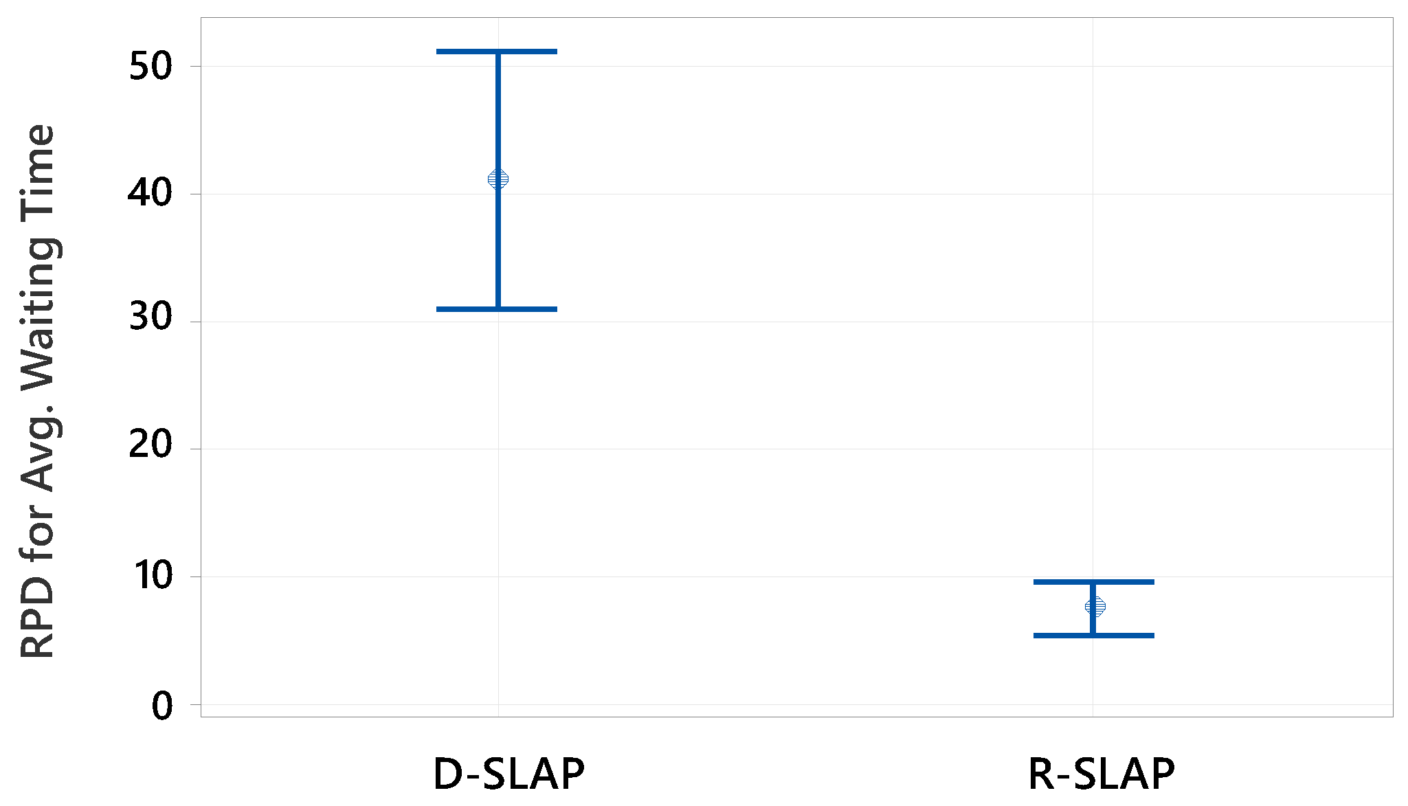
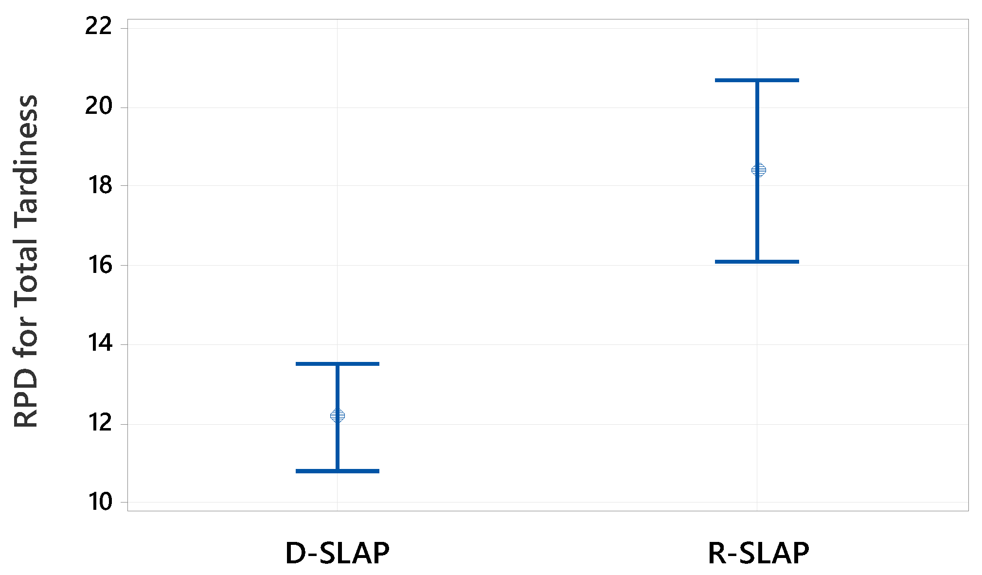
To compare policy performance, interval plots with 95% confidence intervals (CIs) were employed. However, since interval plots rely on aggregated data, they may obscure underlying variability. Therefore, formal hypothesis testing was conducted to rigorously assess the statistical significance of observed differences, accounting for paired data structures and ensuring population-level generalizability. Prior to test selection, normality testing (Shapiro–Wilk test) was performed, where a p-value < 0.05 indicated deviation from normality, necessitating non-parametric alternatives such as the Wilcoxon Signed Rank Test. Normally distributed data justified parametric tests, including the paired t-test.

The RPD was considered for both policies for each of the 24 small and large-size test instances. The best objective value was calculated from each replication’s Pareto front. The differences between the ARPD values of D-DLAP and R-SLAP were calculated for each instance. This resulted in 12 paired differences per objective for each problem size. The Shapiro–Wilk test’s normality tests show different results for the three objectives. For small-sized test instances, the transportation cost shows normality (p-value > 0.100, RJ = 0.956); therefore, a paired t-test is appropriate. The average waiting time has non-normal data (p-value < 0.010, RJ = 0.833), suggesting using a Wilcoxon test. The total tardiness also has non-normal data (p-value < 0.010, RJ = 0.807), indicating the need for a non-parametric test due to non-normality and high variability. For large-size test instances, all three objective functions show approximately normal differences (p-values > 0.100, RJ values of 0.971, 0.979, and 0.965, respectively). This supports the use of a paired t-test for all three objectives. Overall, the differences for all objectives are approximately normally distributed, as indicated by p-values greater than 0.05 and high RJ values, making parametric tests such as the paired t-test suitable for further analysis.

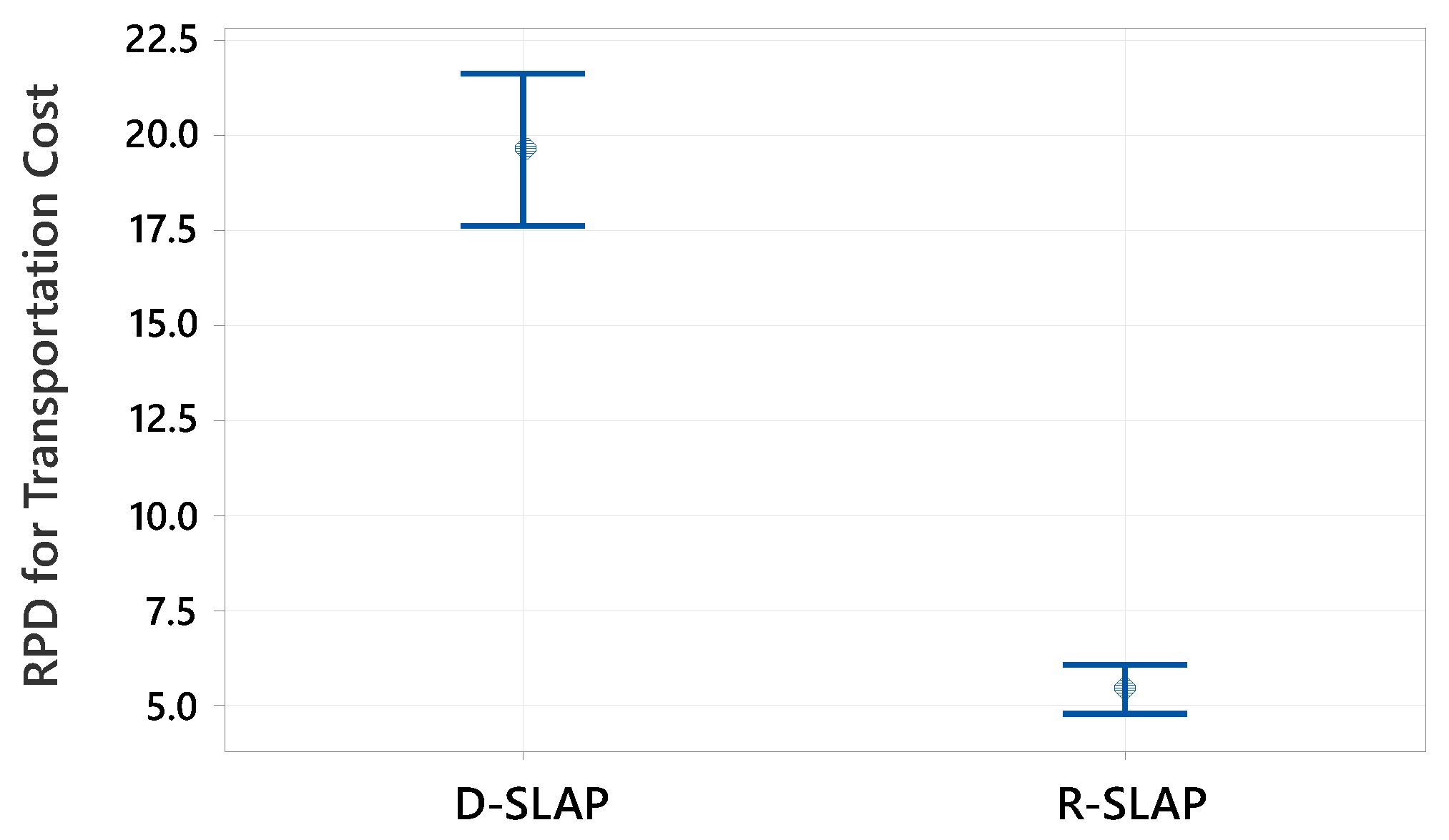
For the transportation cost related to small-size test instances, the paired t-test shows that D-SLAP significantly outperforms R-SLAP, with a mean ARPD difference of −18.81 for H₀: μ_difference = 0 and H₁: μ_difference < 0. For the average waiting time, the Wilcoxon Signed Rank Test shows a significant difference with a p-value of 0.021 and a median difference of 10.8521 for H₀: μ_difference = 0 and H₁: μ_difference > 0. This means D-SLAP performs worse than R-SLAP for this objective. For the total tardiness, the Wilcoxon Signed Rank Test shows a p-value of 0.944, greater than 0.05 for H₀: μ_difference < 0 and H₁: μ_difference ≠ 0. This means there is no significant difference between D-SLAP and R-SLAP, so they perform similarly for this objective.

Regarding the large-size test instances, the paired t-test is applied according to the normality test results of each objective. For the transportation cost, the paired t-test shows that D-SLAP significantly outperforms R-SLAP, with a mean ARPD difference of 14.17 for H₀: μ_difference = 0 and H₁: μ_difference > 0. This supports the results of the interval plot. For average waiting time, the paired t-test shows a significant difference with a p-value of 0.003 and a mean ARPD difference of −4.71 for H₀: μ_difference = 0 and H₁: μ_difference < 0. This means R-SLAP performs better than D-SLAP for this objective. For the total tardiness, the paired t-test shows a p-value of 0.010, less than 0.05 for H₀: μ_difference = 0 and H₁: μ_difference < 0. This means R-SLAP performs better than D-SLAP for this objective. It is worth noting that the choice of the alternative hypotheses is based on the results of the interval plots for the small- and large-sized test instances.

5. Conclusions

This study conducted a comparative analysis of two storage policies, D-SLAP and R-SLAP, to evaluate their impact on warehouse operations, integrating storage allocation with scheduling optimization. A customized NSGA-II metaheuristic was developed, incorporating three solution strings, job sequence, machine assignment, and location assignment, with policy-specific allocation logic. The model addressed multi-objective optimization, minimizing transportation costs, I/O station waiting times, and tardiness, while adhering to precedence, eligibility, and resource constraints. The Taguchi method was employed to optimize metaheuristic parameters for robustness.

This study provides valuable insights for warehouse managers seeking to optimize their operations. Key findings revealed that while both policies generated a similar number of optimal solutions, D-SLAP produced more uniformly distributed Pareto-optimal solutions, advantageous for scenarios requiring diverse alternatives. In contrast, R-SLAP yielded solutions closer to the ideal point, excelling in specific objectives. For small instances, D-SLAP outperformed R-SLAP in minimizing transportation costs. Both policies provide the same performance in terms of the total tardiness, whereas R-SLAP was superior in reducing waiting times. In large instances, R-SLAP dominated in transportation cost minimization, while D-SLAP excelled in waiting time and tardiness reduction. Statistical validation through parametric and non-parametric tests confirmed these performance differences, reinforcing the methodological rigor of the analysis.

From a practical standpoint, warehouse managers should select policies based on operational priorities: D-SLAP for balanced solution diversity and R-SLAP for targeted objective optimization. This research underscores the critical interplay between storage policies and scheduling, offering actionable insights for warehouse efficiency.

Future work should explore hybrid policies to leverage the strengths of both approaches. Additionally, incorporating dynamic supply–demand variability would enhance real-world applicability, while extending the model to include energy-efficient warehousing could address sustainability objectives.

References

1. Wisittipanich, W.; Kasemset, C. Metaheuristics for Warehouse Storage Location Assignment Problems. Chiang Mai Univ. J. Nat. Sci. 2015, 14, 361–377. [Google Scholar] [CrossRef]
2. Waubert de Puiseau, C.; Nanfack, D.T.; Tercan, H.; Löbbert-Plattfaut, J.; Meisen, T. Dynamic Storage Location Assignment in Warehouses Using Deep Reinforcement Learning. Technologies 2022, 10, 129. [Google Scholar] [CrossRef]
3. Bolaños-Zuñiga, J.; Salazar-Aguilar, M.A.; Saucedo-Martínez, J.A. Solving Location Assignment and Order Picker-Routing Problems in Warehouse Management. Axioms 2023, 12, 711. [Google Scholar] [CrossRef]
4. Cai, J.; Li, X.; Liang, Y.; Ouyang, S. Collaborative Optimization of Storage Location Assignment and Path Planning in Robotic Mobile Fulfillment Systems. Sustainability 2021, 13, 5644. [Google Scholar] [CrossRef]
5. Hausman, W.H.; Schwarz, L.B.; Graves, S.C. Optimal Storage Assignment in Automatic Warehousing Systems. Manag. Sci. 1976, 22, 629–638. [Google Scholar] [CrossRef]
6. Gu, J.; Goetschalckx, M.; McGinnis, L.F. Research on Warehouse Design and Performance Evaluation: A Comprehensive Review. Eur. J. Oper. Res. 2010, 203, 539–549. [Google Scholar] [CrossRef]
7. Goetschalckx, M.; Ratliff, D.H. Shared Storage Policies Based on the Duration Stay of Unit Loads. Manag. Sci. 1990, 36, 1120–1132. [Google Scholar] [CrossRef]
8. Manzini, R.; Gamberi, M.; Regattieri, A. Design and Control of an AS/RS. Int. J. Adv. Manuf. Technol. 2006, 28, 766–774. [Google Scholar] [CrossRef]
9. Bartholdi, J.J.; Hackman, S.T. Allocating Space in a Forward Pick Area of a Distribution Center for Small Parts. IIE Trans. 2008, 40, 1046–1053. [Google Scholar] [CrossRef]
10. Quintanilla, S.; Pérez, Á.; Ballestín, F.; Lino, P. Heuristic Algorithms for a Storage Location Assignment Problem in a Chaotic Warehouse. Eng. Optim. 2015, 47, 1405–1422. [Google Scholar] [CrossRef]
11. Larco, J.A.; de Koster, R.; Roodbergen, K.J.; Dul, J. Managing Warehouse Efficiency and Worker Discomfort through Enhanced Storage Assignment Decisions. Int. J. Prod. Res. 2017, 55, 6407–6422. [Google Scholar] [CrossRef]
12. Tang, H.-Y.; Li, M.-J. An Improved Ant Colony Algorithm for Order Picking Optimization Problem in Automated Warehouse. In Fuzzy Information and Engineering Volume 2—Advances in Intelligent and Soft Computing; Cao, B., Li, T.F., Zhang, C.Y., Eds.; Springer: Berlin/Heidelberg, Germany, 2009; Volume 62. [Google Scholar] [CrossRef]
13. Zhang, G.; Shang, X.; Alawneh, F.; Yang, Y.; Nishi, T. Integrated Production Planning and Warehouse Storage Assignment Problem: An IoT Assisted Case. Int. J. Prod. Econ. 2021, 234, 108058. [Google Scholar] [CrossRef]
14. Afzalirad, M.; Rezaeian, J. Resource-Constrained Unrelated Parallel Machine Scheduling Problem with Sequence Dependent Setup Times, Precedence Constraints and Machine Eligibility Restrictions. Comput. Ind. Eng. 2016, 98, 40–52. [Google Scholar] [CrossRef]
15. Heshmati, S.; Toffolo, T.A.M.; Vancroonenburg, W.; Vanden Berghe, G. Crane-Operated Warehouses: Integrating Location Assignment and Crane Scheduling. Comput. Ind. Eng. 2019, 129, 274–295. [Google Scholar] [CrossRef]
16. Tang, L.; Sun, D.; Liu, J. Integrated Storage Space Allocation and Ship Scheduling Problem in Bulk Cargo Terminals. IIE Trans. 2016, 48, 428–439. [Google Scholar] [CrossRef]
17. Fatemi-Anaraki, S.; Tavakkoli-Moghaddam, R.; Abdolhamidi, D.; Vahedi-Nouri, B. Simultaneous Waterway Scheduling, Berth Allocation, and Quay Crane Assignment: A Novel Matheuristic Approach. Int. J. Prod. Res. 2021, 59, 7576–7593. [Google Scholar] [CrossRef]
18. Chen, W.; Zhang, Y.; Zhou, Y. Integrated Scheduling of Zone Picking and Vehicle Routing Problem with Time Windows in the Front Warehouse Mode. Comput. Ind. Eng. 2022, 163, 107823. [Google Scholar] [CrossRef]
19. Zhang, X.; Mo, T.; Zhang, Y. Optimization of Storage Location Assignment for Non-Traditional Layout Warehouses Based on the Firework Algorithm. Sustainability 2023, 15, 10242. [Google Scholar] [CrossRef]
20. Leon, J.F.; Li, Y.; Peyman, M.; Calvet, L.; Juan, A.A. A Discrete-Event Simheuristic for Solving a Realistic Storage Location Assignment Problem. Mathematics 2023, 11, 1577. [Google Scholar] [CrossRef]
21. Antunes, A.R.; Matos, M.A.; Rocha, A.M.A.C.; Costa, L.A.; Varela, L.R. A Statistical Comparison of Metaheuristics for Unrelated Parallel Machine Scheduling Problems with Setup Times. Mathematics 2022, 10, 2431. [Google Scholar] [CrossRef]
22. Gao, X.; Liu, S.; Jiang, S.; Yu, D.; Peng, Y.; Ma, X.; Lin, W. Optimizing the Three-Dimensional Multi-Objective of Feeder Bus Routes Considering the Timetable. Mathematics 2024, 12, 930. [Google Scholar] [CrossRef]
23. Ma, Y.; Li, B.; Huang, W.; Fan, Q. An Improved NSGA-II Based on Multi-Task Optimization for Multi-UAV Maritime Search and Rescue under Severe Weather. J. Mar. Sci. Eng. 2023, 11, 781. [Google Scholar] [CrossRef]
24. Niu, M.; Li, X.; Sun, C.; Xiu, X.; Wang, Y.; Hu, M.; Dong, H. Operation Optimization of Wind/Battery Storage/Alkaline Electrolyzer System Considering Dynamic Hydrogen Production Efficiency. Energies 2023, 16, 6132. [Google Scholar] [CrossRef]
25. Kalra, M.; Singh, S. A Review of Metaheuristic Scheduling Techniques in Cloud Computing. Egypt. Inform. J. 2015, 16, 275–295. [Google Scholar] [CrossRef]
26. Wang, W.; Liu, Y.; Fan, X.; Zhang, Z. Optimization of Charging Station Capacity Based on Energy Storage Scheduling and Bi-Level Planning Model. World Electr. Veh. J. 2024, 15, 327. [Google Scholar] [CrossRef]
27. Morovati, R.; Kisi, O. Utilizing Hybrid Machine Learning Techniques and Gridded Precipitation Data for Advanced Discharge Simulation in Under-Monitored River Basins. Hydrology 2024, 11, 48. [Google Scholar] [CrossRef]
28. Deb, K.; Pratap, A.; Agarwal, S.; Meyarivan, T. A Fast and Elitist Multiobjective Genetic Algorithm: NSGA-II. IEEE Trans. Evol. Comput. 2002, 6, 182–197. [Google Scholar] [CrossRef]
29. Afzalirad, M.; Rezaeian, J. A Realistic Variant of Bi-Objective Unrelated Parallel Machine Scheduling Problem: NSGA-II and MOACO Approaches. Appl. Soft Comput. J. 2017, 50, 109–123. [Google Scholar] [CrossRef]
30. Hidri, L.; Alqahtani, A.; Gazdar, A.; Youssef, B. Ben Green Scheduling of Identical Parallel Machines with Release Date, Delivery Time and No-Idle Machine Constraints. Sustainability 2021, 13, 9277. [Google Scholar] [CrossRef]
31. Larson, R.C.; Sadiq, G. Facility Locations with the Manhattan Metric in the Presence of Barriers to Travel. Oper. Res. 1983, 31, 652–669. [Google Scholar] [CrossRef]
Figure 1. Warehouse layout.
Eng 06 00119 g001
Figure 2. Plot of mean effects of WMPM for NSGA-II.
Eng 06 00119 g002
Figure 3. Plot of mean effects of S/N ratio for NSGA-II.
Eng 06 00119 g003
Figure 4. Plot of obtained Pareto fronts by D-SLAP and R-SLAP for large test instance 2, replication 5.
Eng 06 00119 g004
Figure 5. RPD mean plot and 95% confidence intervals for D-SLAP and R-SLAP for transportation cost using small-size test instances.
Eng 06 00119 g005
Figure 6. RPD mean plot and 95% confidence intervals for D-SLAP and R-SLAP for average waiting time using small-size test instances.
Eng 06 00119 g006
Figure 7. RPD mean plot and 95% confidence intervals for D-SLAP and R-SLAP for total tardiness using small-size test instances.
Eng 06 00119 g007
Figure 8. RPD mean plot and 95% confidence intervals for D-SLAP and R-SLAP for transportation cost using large-size test instances.
Eng 06 00119 g008
Figure 9. RPD mean plot and 95% confidence intervals for D-SLAP and R-SLAP for average waiting time using large-size test instances.
Eng 06 00119 g009
Figure 10. RPD mean plot and 95% confidence intervals for D-SLAP and R-SLAP for total tardiness using large-size test instances.
Eng 06 00119 g010