Determination of Urban Emission Factors for Vehicular Tailpipe Emissions Using Driving Cycles and Cluster-Based Driver Behavior Analysis

Abstract

Urban transportation is a major source of air pollution. On urban highways, driver behavior significantly influences vehicle emissions, as tailpipe pollutants depend on driving patterns. Therefore, estimating the emission factors of key pollutants namely carbon monoxide (CO), carbon dioxide (CO₂), nitrogen oxides (NO_X), and hydrocarbons (HC) is essential. This study investigates the impact of driver behavior on environmental pollutants and derives field-based emission factors on urban highways in Mashhad, Iran, during June 2022. A total of 150 drivers were classified using the K-means algorithm based on their aggressiveness scores from the Driver Behavior Questionnaire (DBQ), maximum acceleration, frequency of maximum acceleration events, and the number of traffic accidents recorded over the past five years. The clustering quality was evaluated using the Silhouette score, leading to two categories: aggressive and non-aggressive drivers. Cochran’s formula was applied to select 10 drivers from each group, and emissions were measured using an onboard monitoring device. Results indicate that aggressive drivers exhibit higher speeds, more pronounced acceleration and deceleration (A/D) patterns, and elevated engine RPM compared with non-aggressive drivers. Spearman’s rank correlation analysis revealed a strong and significant relationship between engine RPM and tailpipe emissions in both driver groups, indicating increased emissions at higher RPMs. In contrast, A/D behavior showed no significant association with emissions, suggesting a minimal direct effect. Overall, emission factors for NO_X, CO₂, CO, and HC were 37.50%, 23.60%, 41.90%, and 53.13% higher, respectively, in aggressive drivers compared with non-aggressive drivers. Furthermore, the Mann–Whitney U test confirmed statistically significant differences in tailpipe emissions between the two groups. These findings demonstrate that distinct driving behaviors are closely linked to variations in vehicular emissions.

1. Introduction

Global data indicate that 92% of the world’s population lives in areas exposed to unsafe levels of air pollution, increasing the risk of diseases such as stroke, heart disease, and lung cancer [1]. Air pollution from various sectors, particularly energy and transportation, continues to rise as urbanization drives growing demands for freight and passenger transport [2,3]. With a population of about 83.9 million, Iran is the most populous country in the Middle East. According to World Bank statistics [4], Iran ranks eighteenth globally in greenhouse gas (GHG) emissions and accounts for 25% of GHG emissions from the transportation sector, primarily due to vehicular exhaust [5]. In urban areas of Iran, passenger vehicles contribute 51%, 37%, and 44% of total exhaust emissions of carbon monoxide (CO), nitrogen oxides (NO_X), and volatile organic compounds (VOCs), respectively, across the entire transportation fleet [6]. The Mashhad Environmental Pollution Monitoring Center in 2022 recorded 70 days with an air quality index rated as “unhealthy for sensitive groups.” Reports further indicate that 70% of Mashhad’s air pollution is attributed to the transportation fleet [7]. Tailpipe emissions consist of a complex mixture of pollutants, with carbon monoxide (CO), carbon dioxide (CO₂), hydrocarbons (HC), and nitrogen oxides (NO_X) being the most critical [8]. Consequently, understanding the effect of driving behavior on tailpipe emissions is crucial [9,10]. On urban highways, driver behavior is influenced by traffic conditions. Such conditions often lead drivers to alternate between normal and aggressive driving modes [11,12]. Moreover, traffic dynamics can alter drivers’ patterns of speed, acceleration, and deceleration (A/D), further affecting emissions [13,14].

Air pollution produced by vehicular traffic under varying driving behavioral characteristics has become a serious concern for traffic engineers and urban authorities. When evaluating air pollution based on tailpipe emissions, it is crucial for policymakers and traffic managers to consider the driving conditions on urban roads. Therefore, traffic and environmental engineers must incorporate driving behavior characteristics into air pollution models to better control vehicular emissions by utilizing emission factors derived from driver behavior. Air pollution models serve as essential tools for traffic and environmental engineers to evaluate urban air quality and predict pollutant levels from vehicles, thereby supporting sustainable urban development goals such as reducing transportation-related emissions. Given the necessity of including driving behavior in such models, this study aims to investigate the effects of driver behavior on tailpipe emissions and to estimate emission factors for present and future applications of air pollution models on urban highways. The findings of this study can assist environmental engineers, transportation planners, and driver-behavior researchers in adopting driver-specific emission factors to improve the accuracy of urban air pollution models.

To propose emission factors for air pollution models based on driver types on urban highways, the study first examines driver behavior characteristics and classifies drivers using the K-means clustering algorithm. The clustering is based on the Driver Behavior Questionnaire (DBQ) scores, maximum acceleration, the frequency of maximum acceleration events, and the number of traffic accidents recorded over the past five years in Mashhad, Iran. After clustering, representative driving cycles were developed for each driver group, which served as the foundation for determining and comparing tailpipe emissions and emission factors across driver types. Finally, on-board measurement equipment was used to collect real-world emission data, including both tailpipe emissions and emission factors for each driver category.

The remainder of this paper is structured as follows: Section 2 presents a comprehensive literature review on assessing the impact of driving behavior on tailpipe emissions. Section 3 details the research methodology, including the evaluation of driver behaviors on urban highways, the classification of drivers using the K-means clustering approach, and the development of driving cycles for each driver type in Mashhad, Iran, followed by the application of on-board measurements to quantify emissions. Section 4 discusses the results and findings derived from the models. Finally, Section 5 concludes the study, highlighting the key results, implications for future research, and the study’s limitations.

2. Literature Review

In this section, previous studies related to driving behavior characteristics and driver classification using the K-means clustering algorithm are reviewed to demonstrate how driver behavior is characterized and categorized based on the Driver Behavior Questionnaire (DBQ) and other driving behavior parameters. Furthermore, studies that evaluate the impact of driving behavior on tailpipe emissions are also presented. The reviewed studies are organized as follows:

2.1. Studies Relevant to Evaluating DBQ and Driving Behavior

The Driver Behavior Questionnaire (DBQ) has been widely applied in numerous studies as a reliable tool for classifying drivers. Lu [15] utilized the DBQ in combination with Principal Component Analysis (PCA) based on real-world driving data to identify driver types. Drivers were classified into five groups: aggressive and non-skillful, prudent and non-skillful, prudent and skillful, aggressive and skillful, and normal. Li et al. [16] applied the standardized DBQ along with a clustering algorithm to classify drivers in Beijing. Their findings revealed that women, older drivers, and those with less driving experience tended to drive more cautiously. Similarly, Gupta [17] validated the DBQ for use in India using exploratory and confirmatory factor analyses, confirming that the DBQ is a robust instrument for assessing aberrant driving behaviors in the Indian context. The study also demonstrated the significant influence of demographic factors on driving behavior, which provides useful insights for improving road safety and traffic management. In a more recent study, Youssef et al. [18] conducted a cross-sectional survey of 1102 Lebanese drivers using the Arabic version of the DBQ. Their results showed that aggressive violations had the highest mean scores, with men more likely than women to commit such violations. The Arabic DBQ version was validated as a reliable and effective tool for assessing aberrant driving behavior.

In addition to questionnaire-based assessments, driving behavior characteristics, particularly speed and acceleration/deceleration (A/D) patterns, have been used as key variables for classifying drivers. Eboli et al. [19] identified unsafe driving behaviors by analyzing speed and A/D data, concluding that these two variables were the most influential in detecting risky driving. Zheng et al. [20] classified drivers into aggressive, conservative, professional, and novice categories using 23 individual driving characteristics, finding that A/D patterns at varying speeds during real-world urban driving tests were critical for classification. Ma et al. [21] further emphasized that many studies rely on speed profiles combined with A/D data from on-board measurement systems to categorize driving styles, noting that aggressive drivers often exhibit A/D values exceeding ±3.5 m/s². Similarly, Ameen [22] proposed a real-time classification method that grouped drivers into safe, normal, aggressive, and dangerous categories based on A/D values, where safe driving corresponded to approximately ±2 m/s², and values above ±4 m/s² indicated aggressive or risky driving.

Beyond behavioral classification, some studies have explored predictive modeling in traffic and mobility contexts. Liu et al. [23] investigated taxi demand prediction in high-demand hotspots using models such as the Random Forest Model (RFM), Ridge Regression Model (RRM), and a Combination Forecasting Model (CFM). Their findings indicated that the CFM outperformed RFM and RRM in terms of robustness and prediction accuracy, particularly when incorporating temporal, weather, and temperature variables. Building on this work, Liu et al. [24] applied a multimodal traffic data approach to enhance online taxi-hailing demand forecasting in metro station areas with different land-use characteristics. They concluded that integrating multisource traffic data significantly improves forecasting accuracy, although prediction performance varies depending on the land-use context surrounding each metro station.

2.2. Studies Relevant to Driver Behavior Classification Using K-Means Clustering

Several studies have investigated driver behavior classification using the K-means clustering algorithm. Jung [25] classified drivers based on both driving behavior and environmental impact using factor analysis combined with K-means clustering. The results indicated that acceleration/deceleration (A/D) patterns and braking behavior had a significant influence on HC, CO, and NO_X emissions. Moreover, defensive and moderate driving styles were found to reduce these emissions compared with speed-focused driving. Similarly, Serttaş et al. [26] analyzed the driving behaviors of 13 individuals using smartphone-based accelerometer and GPS data. They classified drivers into calm, normal, and aggressive groups using the K-means clustering method and achieved the highest accuracy of 93.3% with K = 5, demonstrating the strong potential of K-means for driving style classification. Adamidis et al. [27] proposed a data-driven, simulation-based approach that applied K-means clustering to identify driving profiles based on speed and A/D behavior. Through microscopic traffic simulations, they demonstrated that smooth driving styles and reduced acceleration variability significantly lowered key air pollutant emissions while also improving traffic network efficiency.

In another study, Mohammadnazar et al. [28] examined the impact of driving volatility on emissions in critical roadway sections such as work zones and sharp curves. Using K-medoids and hierarchical clustering, they classified driving styles and found that aggressive driving accounted for 12.2% of events in work zones and 15.4% on curves compared with normal driving. Du et al. [29] applied K-means clustering alongside K-medoids and Principal Component Analysis (PCA) for dimensionality reduction to group driver behavioral indicators obtained from GPS data. Their clustering approach enabled a deeper analysis of the relationship between driver behavior types and traffic emissions, facilitating better prediction and management of pollutant outputs. Lastly, Almachi et al. [30] utilized the K-means clustering algorithm to develop a representative urban driving cycle for Quito, Ecuador. They constructed a 2870-s driving cycle that effectively captured the city’s distinctive traffic characteristics, which were influenced by frequent A/D variations caused by the linear urban road structure.

2.3. Studies on the Impact of Driver Behavior on Tailpipe Emissions

Several studies have investigated the effect of driving behavior on tailpipe emissions. Nam et al. [31] examined the modeling of emissions under varying levels of driver aggressiveness using on-board measurement systems, traffic simulation, and speed and acceleration/deceleration (A/D) behavior. Their results showed that the developed model closely matched on-board measurements and confirmed that aggressive driving naturally leads to significantly higher emissions. Other researchers have also developed behavior-based models to estimate exhaust emissions on urban highways by incorporating speed and A/D patterns, demonstrating that such models can reliably predict emissions under real-world driving conditions [32,33,34]. Carrese et al. [35] specifically focused on bus drivers and found that driver behavior significantly influences CO and NO_X emissions. In a related study, Zheng et al. [36] analyzed the car-following behavior of 28 drivers in Chengdu, China, using GPS data, acceleration profiles, accident history, and DBQ scores to classify drivers into four categories: macho, careful/inexperienced, smooth/professional, and experienced/fast. Their findings revealed substantial differences in emissions across these driver types. Huang et al. [37] assessed emissions using on-board measurements to compare professional and novice drivers. The study found that NO_X and PM emissions by novice drivers were 17% and 29% higher, respectively, than those of professional drivers. Suarez et al. [38] developed an acceleration-aggressiveness metric to quantify the effect of real-world heterogeneous driving on CO₂ emissions, reporting a clear increase in CO₂ emissions with rising acceleration aggressiveness. Chandrashekar et al. [39] evaluated the real-world emissions of diesel passenger cars in heterogeneous traffic conditions in India using on-board measurement and speed/A/D data to compare aggressive and normal drivers. They reported that aggressive driving increased CO, HC, and CO₂ emission factors by 5–25% compared with normal driving on both urban and rural roads. Moreover, NO_X emission factors were also found to be significant under normal driving conditions in urban settings. Jia et al. [40] combined real-world trajectory data and machine learning to evaluate how Intelligent Transportation Speed Guidance Systems (ITSGS) reduce vehicle emissions. By applying K-means clustering to identify driving styles, such as aggressive, moderate, and smooth, they demonstrated that smoother driving significantly lowers CO₂, NO_X, CO, and HC emissions, highlighting the long-term environmental benefits of ITSGS. Despite this extensive body of research, no prior study has classified driver behavior on urban highways to determine emission factors for CO, CO₂, NO_X, and HC using on-board measurement methods. Thus, the novelty of the present study lies in applying K-means clustering to classify driver behavior based on the DBQ, maximum acceleration, number of maximum acceleration events, and five-year traffic accident history for drivers on urban highways in Mashhad, Iran, as a case study focusing on Iranian drivers. Furthermore, this study investigates the impact of engine RPM and A/D behavior on the tailpipe emissions of passenger vehicles across different driver types.

3. Research Method

To investigate the influence of driver behavior on tailpipe emissions and to estimate emission factors using on-board measurements on urban highways, the research procedure is illustrated in Figure 1. The study began with the selection of 150 male drivers employed by Snapp, a major ride-hailing and online transportation service provider in Iran (comparable to Uber). Data collection was conducted on urban highways in Mashhad, Iran, during June 2022. According to the statistical yearbook of the planning and development department of the municipality of Mashhad [41], Mashhad, with a population of 3,315,000 residents, experienced a 2.10% population increase since 2021. Reports estimate approximately 6,657,765 daily trips within the city [42], a substantial figure compared with other Iranian cities. This growth is largely attributed to the rising urban population and the influx of religious tourists, which has placed significant pressure on the urban transportation network [43]. Consequently, Mashhad has faced serious environmental challenges related to emissions from passenger vehicles [44]. Hence, assessing air quality impacts from light-vehicle exhaust emissions in this city is of critical importance.

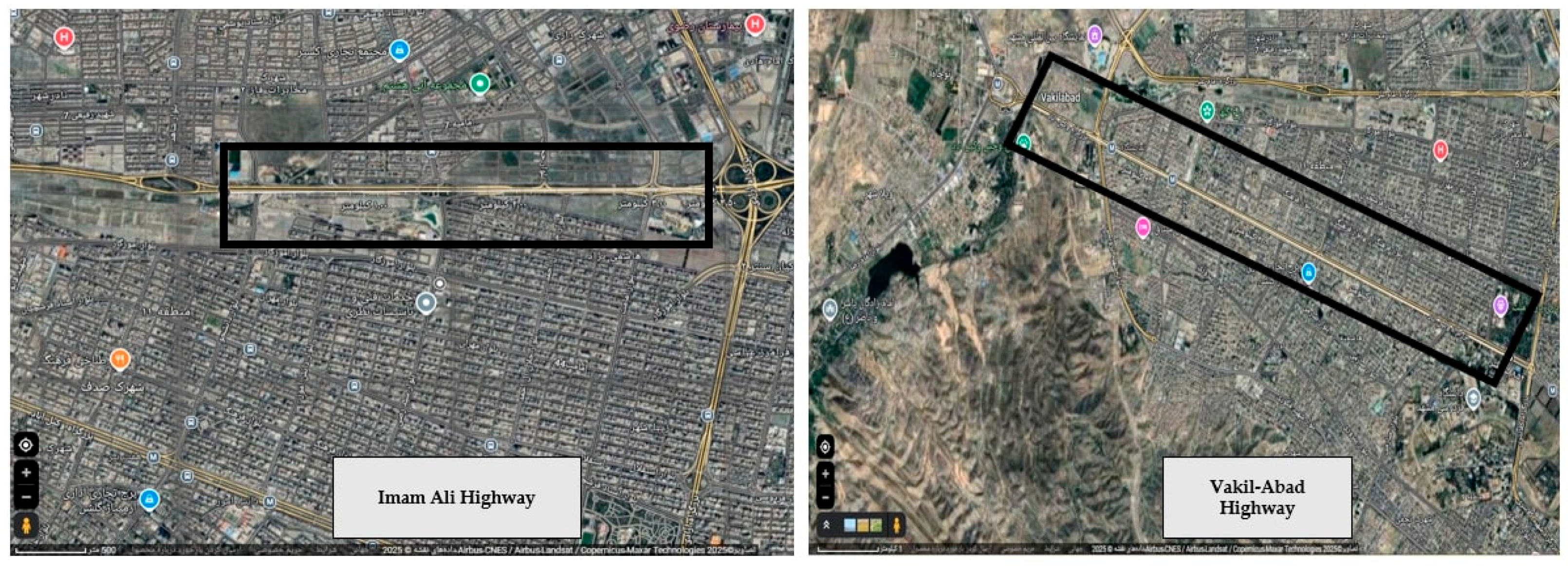
In the first step, speed and acceleration/deceleration (A/D) data were recorded at a 1 Hz frequency using a GPS device. Following the trips, drivers completed the Driver Behavior Questionnaire (DBQ) to self-report their aggressiveness scores. Four key parameters, aggressiveness score, maximum acceleration, number of maximum acceleration events, and number of traffic accidents over the past five years (June 2017–June 2022) were selected as primary behavioral indicators. The Hopkins statistic was employed to evaluate the clusterability of the dataset. Subsequently, the K-means clustering algorithm was applied, and the Silhouette score was used to assess clustering quality. To enhance computational efficiency and minimize redundancy, the data were standardized and reduced using Principal Component Analysis (PCA). Following clustering, a representative driving cycle was developed for each cluster to capture the distinct behavioral characteristics of drivers within each group. Finally, tailpipe emissions and emission factors for CO, CO₂, NO_X, and HC were obtained using the on-board measurement method with AVL DiTEST MDS 215 [45] gas analyzer for a sample of 10 drivers from each cluster. Figure 2 shows the selected study highways in Mashhad, Iran. A 12-km straight, longitudinal segment covering Imam Ali and Vakil-Abad highways, each featuring three lanes of 3.65 m width, was chosen to minimize the influence of longitudinal slope, intersections, and horizontal alignments on the experiments. All speed and A/D data were collected under clear daylight conditions during June 2022, specifically in the time intervals of 7:30–9:00 a.m. and 4:00–6:00 p.m. Test trips were conducted under both congested and uncongested traffic conditions, and the posted speed limit on the study highways was 90 km/h during daylight.

3.1. Selecting Driving Parameters for Cluster Analysis

In the present analysis, four key parameters were selected for the cluster analysis: aggressiveness score (calculated as the average score from the DBQ), maximum acceleration, number of maximum acceleration events, and number of traffic accidents recorded over the past five years. The DBQ consisted of 23 items designed to assess drivers’ tendencies toward aggressive driving behaviors (

Table A1. DBQ survey.

Number	Description	Never	Occasionally	Quite	Frequently	Always
1	Deliberately disregard the speed limits late at night or very early in the morning.
2	Get involved in unofficial ‘races’ with other drivers.
3	Overtake a slow-moving vehicle on the inside lane or hard shoulder of a motorway.
4	Become impatient with a slow driver in the outer lane and overtake on the inside.
5	Race oncoming vehicles for a one-car gap on a narrow or obstructed road.
6	Overtake a single line of stationary or slow-moving vehicles, only to discover that they were queuing to get through a one-lane gap or roadwork lights.
7	Deliberately drive the wrong way down a deserted one-way street.
8	Take a chance and cross on lights that have turned red.
9	Drive as fast along country roads at night on dipped lights as on full beam.
10	Drive especially close or ‘flash’ the car in front as a signal for that driver to go faster or get out of your way.
11	Stuck behind a slow-moving vehicle on a two-lane highway, you are driven by frustration to try to overtake in risky circumstances.
12	Fail to give way when a bus is signaling its intention to pull out.
13	Have an aversion to a particular class of road user, and indicate your hostility by whatever means you can.
14	Angered by another driver’s behavior, you give chase with the intention of giving him/her a piece of your mind.
15	Misjudge your crossing interval when turning right and narrowly miss collision.
16	Fail to notice pedestrians crossing when turning into a side street from a main road.
17	Misjudge speed of oncoming vehicle when overtaking.
18	Fail to notice someone stepping out from behind a bus or parked vehicle until it is nearly too late.
19	Hit something when reversing that you had not previously seen.
20	In a queue of vehicles turning left onto a main road, pay such close attention to the traffic approaching from the right that you nearly hit the car in front.
21	Attempt to overtake a vehicle that you hadn’t noticed was signaling its intention to turn right.
22	Lost in thought or distracted, you fail to notice someone waiting at a zebra crossing, or a pelican crossing light that has just turned red.
23	Misread signs and take the wrong exit from a roundabout.

in Appendix A). Each item was rated on a 5-point Likert scale ranging from 1 (“Never”) to 5 (“Always”) [46], with higher scores indicating stronger aggressive tendencies. To capture additional behavioral nuances, drivers were asked to complete the DBQ using a Likert-type scale, where 0 denotes no tendency toward a given behavior and 5 indicates the strongest tendency [47]. The questionnaire was administered to all 150 participating drivers. For each participant, an overall aggressiveness score was computed by averaging their responses across all 23 items. This average score was then included as one of the key input features in the K-means clustering algorithm to classify drivers based on their behavioral profiles.

To ensure the reliability of the survey instrument, the internal consistency (α) of the DBQ was evaluated. According to Cronbach [48], Cronbach’s alpha is a function of the number of items in the test, the average covariance between item pairs, and the variance of the total score. In this study, the calculated Cronbach’s alpha was 0.759 based on the responses of the 150 drivers, indicating an acceptable level of reliability for the DBQ.

3.2. Hopkins Statistic Analysis for Data Suitability

According to Banerjee and Dave [49], the Hopkins statistic is a robust indicator of cluster tendency: values near 0.5 suggest randomness, values approaching 1.0 indicate a strong tendency to form clusters, and values below 0.5 imply a uniform or anti-clustered distribution. In the present study, before performing the K-means clustering analysis, the Hopkins statistic was computed using 10 random iterations with a sampling ratio of 10% to evaluate the inherent cluster tendency of the dataset. The obtained value of 0.7663 ± 0.0423 demonstrates a substantial deviation from randomness, confirming a meaningful tendency for the data to form clusters. This result supports the validity of applying centroid-based clustering methods such as K-means. The statistic was calculated prior to dimensionality reduction with PCA, indicating that the dataset inherently exhibits a strong clustering structure, providing a suitable foundation for the K-means algorithm.

3.3. Selecting the Number of Clusters Using the Silhouette Coefficient

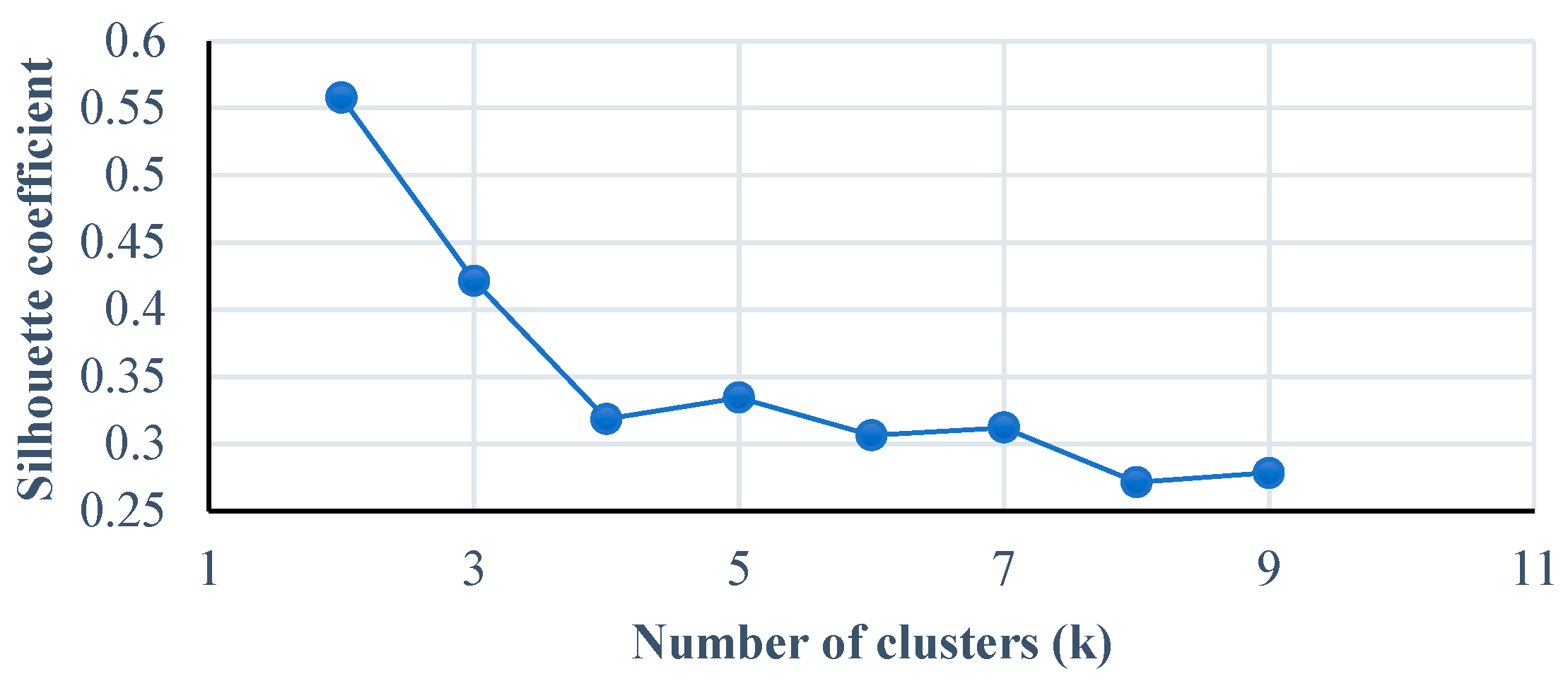
To identify the optimal number of clusters (k), the silhouette coefficient was calculated as a measure of cluster separation quality. Based on this metric (Figure 3), the optimal number of clusters was determined to be k = 2. Consistent with Zheng et al. [36], drivers with higher maximum acceleration, a greater number of accidents, and higher aggressiveness scores were identified as “aggressive” drivers, while those with lower values for these characteristics were categorized as “non-aggressive.” The classification results are summarized in

Table A2. Summary of key attributes per cluster (K-means results) for aggressive drivers.

Driver Id	Average Score	Maximum Acceleration	Number of Maximum Acceleration Events	Number of Accidents
2	2.05	1.71	6	14
47	2.12	1.79	7	11
66	1.97	1.56	7	14
93	2.02	1.62	6	13
96	1.97	1.70	7	12
105	2.03	1.65	7	14
131	2.00	1.60	7	12
133	2.09	1.82	6	11
145	2.02	1.70	7	12
148	2.01	1.87	5	11

and

Table A3. Summary of key attributes per cluster (K-means results) for non-aggressive drivers.

Driver Id	Average Score	Maximum Acceleration	Number of Maximum Acceleration Events	Number of Accidents
1	1.69	1.60	0	4
4	1.71	1.30	4	3
19	1.57	1.55	1	2
30	1.65	1.63	2	1
45	1.63	1.35	2	4
46	1.57	1.69	0	3
126	1.68	1.46	2	3
134	1.66	1.59	2	3
136	1.68	1.46	1	4
146	1.63	1.63	2	1

in Appendix A.

3.4. Applying PCA for Cluster Validation on the Dataset

Prior to applying PCA and K-means clustering, all input features were standardized using z-score normalization through the standard scaler method. This preprocessing step ensured that each feature contributed equally to the formation of principal components and clustering results, thereby preventing dominance by features with larger numeric ranges. Principal Component Analysis (PCA) was then applied to reduce the four-dimensional feature space into two principal components for both dimensionality reduction and cluster validation. The first two principal components together explained 85.06% of the total variance, ensuring that most of the original data characteristics were preserved and allowing for effective visualization of the clusters. The K-means clustering performed on the PCA-transformed dataset achieved a silhouette score of 0.6608, indicating well-defined and clearly separated clusters. A silhouette score above 0.5 is generally considered evidence of reliable and meaningful cluster detection [50].

3.5. Identification of Drivers from Clusters

In this study, the Cochran formula was employed to estimate the required sample size for field data collection. To apply the formula, preliminary fieldwork was conducted by manually counting vehicles with a 1503 cc engine passing through the target highways. Observations revealed that, on average, 35 vehicles passed each hour, of which approximately 18 were driven by male drivers. Using this observed proportion and a 5% margin of error, the required sample size for male drivers of 1503 cc vehicles was calculated to be approximately 20. A detailed summary of participant characteristics is presented in

Table 1. Detailed summary of participant characteristics.

Variables	Group	Number	Percentage
Gender	Male	20	100
Age (year)	18–26	3	15%
	27–30	4	20%
	31–36	6	30%
	37–45	2	10%
	>45	5	25%
Driving experience (year)	1–4	5	25%
	5–8	2	10%
	9–12	3	15%
	13–18	3	15%
	>18	7	35%
Employment type	Permanent	14	70%
	Temporary	6	30%
Number of accidents in the past five years (2017–2022)	0–3	3	15%
	3–6	7	35%
	6–9	0	0%
	9–12	3	15%
	12–15	7	35%

. As shown in Table 1, all participants were male drivers aged 18–52 years. Most participants were relatively young, had more than 18 years of driving experience, considered driving as their primary occupation. From the classified drivers, 10 representative samples from each cluster were selected based on the Euclidean distance of each driver to the cluster center in the K-means model. Drivers closest to the cluster center were chosen to best represent the characteristics of each group. These representative samples were then used for further analyses and evaluations of driving behaviors.

To examine whether age or driving experience influenced the driver classifications, statistical tests were performed for both variables, and the results are summarized in

Table A4. Statistical tests for age and driving experience.

Variable	Test	Statistic	p-Value	Sig. (2-Tailed)
Age	Shapiro–Wilk (Aggressive)	0.935	0.497	Not significant
	Shapiro–Wilk (Non-aggressive)	0.928	0.426	Not significant
	Independent t-test	−0.336	0.741	Not significant
Driving experience	Shapiro–Wilk (All)	0.9117	0.0687	Not significant
	Independent t-test	0.0177	0.9860	Not significant

. The Shapiro–Wilk test confirmed that both clusters were normally distributed, and the independent t-test revealed no significant differences in age or driving experience between the clusters. Consequently, these variables, along with gender and driving experience, were excluded from the clustering process due to their lack of significant influence on driver type. The analysis of the two clusters revealed distinct behavioral profiles. Drivers in Cluster 1 exhibited higher mean values across all key behavioral indicators compared to those in Cluster 0, with a maximum acceleration of 1.87 m/s² versus 1.69 m/s², an average of 6.50 versus 1.60 maximum acceleration events, and 12.40 versus 2.80 accidents over five years. These results indicate that Cluster 1 represents aggressive drivers, characterized by higher acceleration, more frequent extreme driving events, and a greater accident history, while Cluster 0 represents non-aggressive drivers, displaying consistently lower values across these parameters. This finding aligns with the observations of Zheng et al. [36], who reported that drivers with aggressive tendencies generally exhibit higher DBQ scores, more extreme acceleration patterns, and a greater number of accidents. A summary of these representative samples is presented in Table A2 and Table A3 in Appendix A.

3.6. Operational and Environmental Conditions for AVL DiTEST MDS 215 MDS Emission Testing

The conditions for using the AVL DiTEST MDS 215 device (Graz, Austria) [45] and the conditions under which the measurements were conducted are described as follows:

• Filter maintenance: The filters of the AVL DiTEST MDS 215 device were cleaned to ensure that the gas pathways were not blocked, in accordance with the AVL DiTEST MDS user manual [45].
• Stabilization time: The device was turned on 15 min prior to testing to allow the sensors to stabilize before measurements began [45].
• Environmental conditions: The device was operated in a stable environment with controlled room temperature and humidity throughout the measurement period.
• Sunlight protection: The device was kept away from direct sunlight to avoid sensor interference and ensure accurate readings [45].
• Fuel quality: All vehicles tested used Euro-4 petrol to eliminate variations in fuel quality and minimize its influence on emission levels.
• Testing environment: The tests were conducted under controlled temperature, humidity, and pressure to maintain consistent measurement conditions.
• Weather conditions: The average ambient temperature during the test period was approximately 26 °C, and the relative humidity was 37%. Testing was avoided on days with strong winds or rainfall to ensure stable conditions for measurements.
• Altitude of Mashhad: The altitude of Mashhad (950 m above sea level) was considered in the analysis because altitude can significantly influence vehicle emissions [51].
• Air-conditioning settings: To prevent the vehicle’s air-conditioning (AC) system from affecting emission levels, AC settings were kept constant in all vehicles during the tests [52].
• Vehicle start mode: Cold-start conditions were excluded from this study, as engines were warmed up before testing. Cold starts typically result in higher emission factors because more energy is required to heat the engine compared to a hot start. The off-time of the vehicle can also influence cold-start emissions; therefore, by starting measurements only after the engine warmed up, this effect was minimized [53].

3.7. Fuel Characteristics

The physical quality of fuel is a crucial factor influencing the emission factor of vehicles. Key fuel characteristics include its type (petroleum-based) and its chemical content, such as sulfur, lead, benzene, oxygen, and other additives. According to a report by the Mashhad Oil Products Distribution Company, the sulfur and benzene contents of the fuel used in this study were at the upper regulatory limits, 600 ppm and 3%, respectively, while the amounts of oxygen and lead were negligible (close to zero). The test vehicles were typical light passenger cars widely used by drivers in the Snapp Company, including Tiba, Saina, and Quik models, with model years ranging from 2015 to 2022. These vehicles weighed less than 5000 lbs (around 2268 kg) and had accumulated mileage in the range of 40,000–80,000 km. Additional vehicle characteristics, including emission control technologies, are provided in

Table 2. General emission control and emission characteristics of test vehicles.

Evaporative Control	Exhaust Control	Air/Fuel Control	Engine Size	Fuel	Cylinders	Valves per Cylinder	Engine Power (hp)	Torque (Nm)
Positive crankcase ventilation	Three-way	Multipoint fuel injection	Medium	Petroleum	4	2	87	128

and

Table A5. Detailed engine characteristics of test vehicles.

Driver ID	Mileage (km)	Engine Volume (cc)	Fuel Type	Emission Standard	Tire Age (Months)	Last Service Date
Driver_1	40,839	1503	Petroleum	Euro 4	12	12/2021
Driver_2	41,756	1503	Petroleum	Euro 4	6	02/2022
Driver_3	75,493	1503	Petroleum	Euro 4	28	11/2021
Driver_4	78,520	1503	Petroleum	Euro 4	32	01/2022
Driver_5	61,361	1503	Petroleum	Euro 4	15	12/2021
Driver_6	67,536	1503	Petroleum	Euro 4	10	01/2022
Driver_7	49,257	1503	Petroleum	Euro 4	8	02/2022
Driver_8	58,312	1503	Petroleum	Euro 4	16	11/2021
Driver_9	56,936	1503	Petroleum	Euro 4	14	12/2021
Driver_10	54,033	1503	Petroleum	Euro 4	12	01/2022
Driver_11	67,870	1503	Petroleum	Euro 4	30	11/2021
Driver_12	48,009	1503	Petroleum	Euro 4	5	02/2022
Driver_13	58,327	1503	Petroleum	Euro 4	18	12/2021
Driver_14	79,989	1503	Petroleum	Euro 4	34	11/2021
Driver_15	78,331	1503	Petroleum	Euro 4	36	01/2022
Driver_16	74,241	1503	Petroleum	Euro 4	24	12/2021
Driver_17	61,296	1503	Petroleum	Euro 4	6	02/2022
Driver_18	51,364	1503	Petroleum	Euro 4	10	01/2022
Driver_19	40,979	1503	Petroleum	Euro 4	8	12/2021
Driver_20	46,912	1503	Petroleum	Euro 4	9	11/2021

in Appendix A. All vehicles were equipped with positive crankcase ventilation (PCV), which connects the crankcase to the engine’s air intake to create negative pressure, drawing volatile organic compounds (VOCs) into the combustion chamber for incineration alongside the fuel.

To reduce harmful exhaust pollutants, each vehicle used a three-way catalytic converter that lowers CO, VOCs, and NO_X emissions. The engines also utilized a multipoint fuel injection system in which fuel is injected directly into the engine cylinders just ahead of the valves or injectors, enabling precise control of the air-fuel mixture. The vehicles had similar engine specifications, including a 1.5-L, 4-cylinder engine rated at 87 horsepower (hp) and were fueled with Euro 4-compliant petrol. According to Table 2 and Table A5 in Appendix A, all 20 vehicles belonged to Snapp’s operational fleet and were subject to strict company regulations mandating regular technical inspections and emission system checks to ensure proper maintenance. Drivers were prohibited from operating vehicles or providing passenger services unless all required inspections and maintenance were up to date. Therefore, Table 2 and Table A5 summarize each vehicle’s mileage, engine volume, fuel type, emission standard, and vehicle type (single fuel), offering a comprehensive overview of the fleet characteristics used in this study to evaluate the effect of driver behavior on vehicular emissions.

3.8. Estimation of Tailpipe Emissions via On-Board Measurement

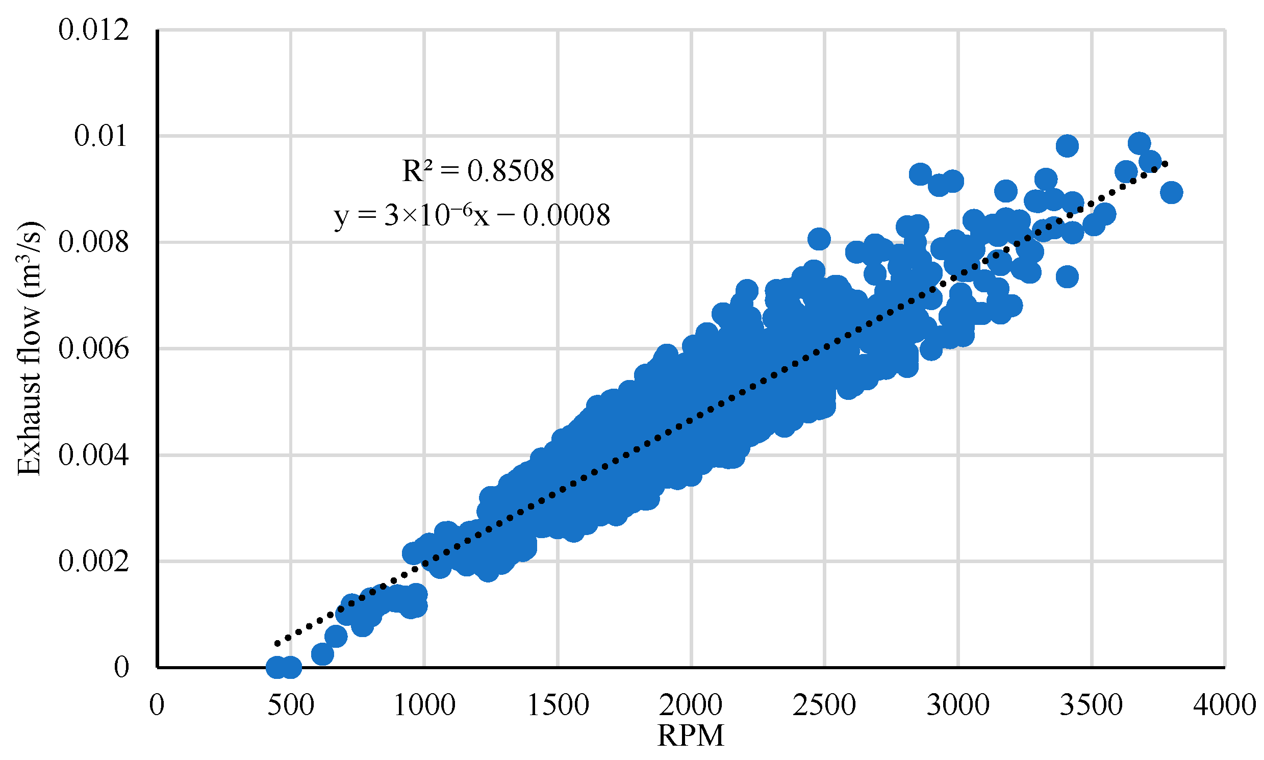
In this study, on-board emissions were measured for 10 drivers from each of the identified driver groups, aggressive and non-aggressive. To evaluate the impact of driving behavior on vehicle emissions, the calculations were performed using Equations (1)–(4), in which one of the key parameters is the exhaust flow rate (Q_exhaust, m³/s). Accurate estimation of Q_exhaust was therefore critical to determine the emission factors using on-board measurements. To establish the relationship between engine speed (RPM) and exhaust flow rate, data were collected from the Center of Purification of Mashhad for 30 min for a representative light vehicle that matched the specifications outlined in Table 1. It should be noted that this 30-min dataset (Figure 4) was selected from a larger dataset originally recorded over 300 min (5 h). The full dataset comprised measurements from 30 different vehicles (Tiba and Saina, 1503 cc), while the selected 30-min segment represents a single vehicle. The representative segment was chosen based on the relative error criterion, ensuring that the average value of Q_exhaust within this 30-min period deviated by no more than 3% from the overall mean of the entire 300-min dataset. As a result, the selected vehicle was deemed representative of the 30-vehicle fleet. A linear equation was then developed from these data to describe the relationship between RPM and Q_exhaust, demonstrating good prediction performance (Figure 4). Once the relationship was established, the real-world RPM data for both aggressive and non-aggressive drivers were substituted into the derived equation to obtain exhaust flow rates for each driver group. Tailpipe emissions were subsequently calculated for both groups using Equations (1)–(4), which convert the measured exhaust emissions of passenger vehicles into grams per second (g/s) [54].

To validate the exhaust flow rate estimates, the observed and predicted Q_exhaust values were compared as a function of engine speed (RPM), and the results were plotted in Figure A1 of Appendix A. As shown in Figure A1, the predicted and observed flow rates were in close agreement, with differences remaining within an acceptable range. The coefficient of determination (R² = 0.85) confirmed a strong correlation between observed and predicted values, demonstrating that the derived Q_exhaust relationship is reliable for the present study.

$$CO(g/s)=Q_{exhaust}\times {\displaystyle \frac{M_{CO}\times {CO}_{\%}\times {10}^{-2}}{0.0283}}.$$

(1)

$$HC(g/s)=Q_{exhaust}\times {\displaystyle \frac{M_{HC}\times H{C}_{PPM}\times {10}^{-6}}{0.0283}}.$$

(2)

$$N{O}_X(g/s)=Q_{exhaust}\times {\displaystyle \frac{M_{{NO}_X}\times {NO}_{XPPM}\times {10}^{-6}}{0.0283}}.$$

(3)

$$C{O}_2(g/s)=Q_{exhaust}\times {\displaystyle \frac{M_{C{O}_2}\times {CO}_{2\%}\times {10}^{-2}}{0.0283}}.$$

(4)

In Equations (1)–(4), M_CO (g/mol), M_CO2 (g/mol), M_NOx (g/mol), and M_HC (g/mol) denote the molar masses of CO, CO₂, NO_x, and HC, respectively. In the above equation, M_CO2, M_CO, M_NOx, and M_HC represent the molar masses of carbon dioxide (CO₂), carbon monoxide (CO), nitrogen oxide (NO_X), and hydrocarbon (HC). In addition, Q_exhaust (m³/s) represents the discharge of exhaust gas. After obtaining the amounts of CO, CO₂, NO_x, and HC in g/s, the average emission factor can be calculated using Equation (5):

$$Emission \mathrm{factor} (\mathrm{g}/\mathrm{km}) ={\displaystyle \frac{3600\times {\displaystyle \sum _t^n{e}_t}}{{\displaystyle \sum _t^n{V}_t}}} ,$$

(5)

where e_t is the tailpipe emission (g/s), and V_t is the corresponding vehicle speed at time t (km/h).

3.9. Determining the Driving Cycle for Driver Behavior

In the present study, K-means clustering was employed to classify drivers based on four key parameters: aggressiveness score, maximum acceleration, number of maximum acceleration events, and number of traffic accidents. From each cluster, 10 representative drivers, 10 aggressive and 10 non-aggressive, were selected based on their Euclidean distance to the cluster centers, ensuring that the chosen drivers best represented the behavioral profiles of each group. To compare the tailpipe emissions and emission factors between these two driver groups, emissions were calculated and analyzed according to the driving cycle developed for each group. To establish the driving cycles that reflect the behavior of each driver group, approximately 500 micro-trips were analyzed using speed-time data collected from the 10 aggressive and 10 non-aggressive drivers. Based on these micro-trips, two distinct driving cycles were developed, each representing the characteristic driving patterns of its respective group. The cycles were constructed by randomly combining micro-trips until the desired driving cycle length was achieved. The length of the driving cycle varies depending on the characteristics of the trips and typically ranges between 900 and 1400 s [55]. To assess the accuracy of the developed driving cycles for Mashhad’s urban highways, the relative error was calculated using Equation (6) for the following key parameters: mean speed, mean speed while moving, mean acceleration (a > 0), mean deceleration (a < 0), percentage of time with zero acceleration (cruise mode), percentage of time with acceleration, percentage of time with deceleration, percentage of time at zero speed, and the root mean square (RMS) of acceleration [55].

$$\left|{\displaystyle \frac{P_t-p_i}{p_t}}\right|<0.05.$$

(6)

In Equation (6), $P_t$ denotes the parameter value calculated from the entire dataset, while $P_i$ represents the corresponding parameter value derived from the developed driving cycle.

Table 3. The error rate for each parameter in the driving cycle.

Driver Type	Aggressive Driver			Non-Aggressive Driver
Parameter	Pt	Pi	Relative Error (%)	Pt	Pi	Relative Error (%)
Mean speed	40.54	41.15	1.50	34.27	35.77	4.38
Mean speed while moving	45.76	43.97	3.91	36.42	37.92	4.12
Mean acceleration	0.53	0.52	1.89	0.45	0.47	4.44
Mean deceleration	−0.54	−0.53	1.85	−0.56	−0.58	3.57
% Time cruise mode	11.05	10.68	3.35	10.06	10.34	2.78
% Time acceleration	43.75	44.44	1.58	48.21	49.95	3.61
% Time deceleration	43.92	44.88	2.19	38.98	39.72	1.90
% Time speed = 0	6.73	6.43	4.46	5.77	5.66	1.91
RMS acceleration	0.61	0.64	4.92	0.62	0.63	1.61

Note. RMS: Root mean square.

presents the error rates for each parameter by comparing $P_i$ and $P_t$. Since all error rates are less than 5%, the proposed driving cycles are deemed to accurately represent both aggressive and non-aggressive drivers operating on urban highways.

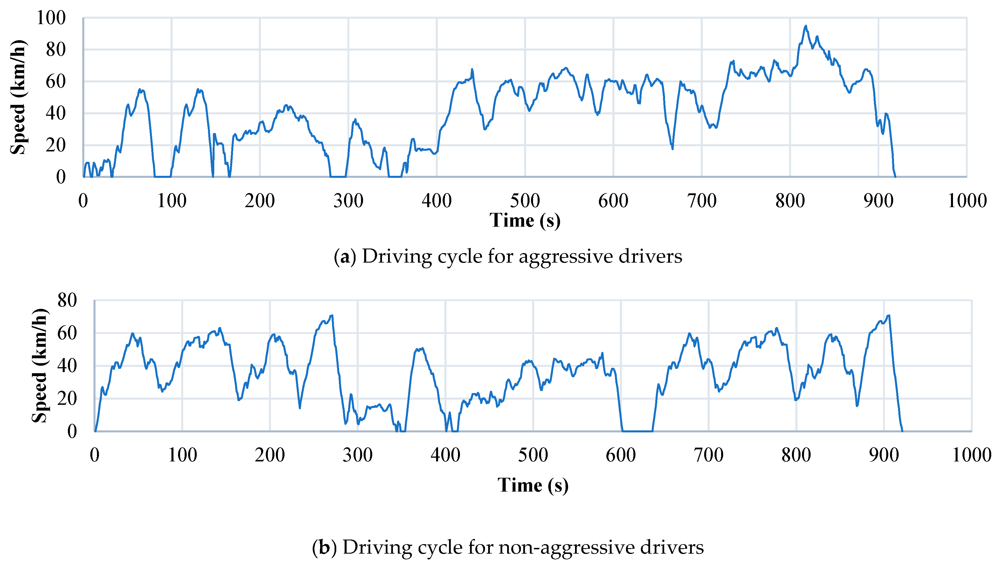
Figure 5 illustrates the driving cycles of aggressive and non-aggressive drivers, highlighting the behavioral distinctions between the two groups. As shown in Figure 5a,b, the maximum speed in the aggressive driving cycle reached 91 km/h, compared to 70 km/h in the non-aggressive cycle, indicating that aggressive drivers tend to drive at higher speeds. The higher speeds observed in aggressive drivers contribute to more pronounced stop-and-go traffic patterns and increased braking events. This is further reflected in the percentage of time spent decelerating, which is higher for aggressive drivers (43.92%) compared to non-aggressive drivers (38.98%). Similarly, Table 3 shows that the mean speed and mean acceleration are greater for aggressive drivers (mean speed: 40.54 km/h; mean acceleration (a > 0): 0.53 m/s²) than for non-aggressive drivers (mean speed: 34.27 km/h; mean acceleration (a > 0): 0.45 m/s²). These results underscore the more variable and dynamic driving patterns of aggressive drivers, which lead to greater traffic oscillations and more frequent braking events compared to non-aggressive drivers.

4. Results and Discussion

This section presents the results of tailpipe emissions in relation to driver behavior type using on-board measurements obtained from 10 aggressive and 10 non-aggressive drivers. Statistical comparisons between the two groups were carried out using the Mann–Whitney U test, while Spearman’s rank correlation was employed to examine the relationships between engine RPM and tailpipe emissions, as well as between acceleration/deceleration (A/D) behavior and tailpipe emissions. Finally, emission factors were calculated for both driver groups.

4.1. Pollutant Results Based on Driver Behavior

After classifying the drivers using the K-means clustering algorithm, tailpipe emissions were calculated for each driver group based on on-board measurement data collected over a 920-s driving cycle. The calculation followed Equations (1)–(4), and the results of the initial statistical analysis are provided in

Table 4. Statistical analysis of Q_exhaust (m/s³) and tailpipe emissions (g/s) for driver type.

Driver Type	Parameter	Minimum	Maximum	Mean	SD	Variance	Std Error of Mean	%CV
Aggressive	Qexhaust	0.0016	0.0128	0.0076	0.0027	0.0000	0.0000	35.53
	CO2	0.4403	3.7583	2.0795	0.7819	0.6113	0.0258	37.60
	CO	0.0290	0.2660	0.1398	0.0525	0.0028	0.0017	37.55
	NOX	0.0004	0.0037	0.0018	0.0007	0.0000	0.0000	38.89
	HC	0.0001	0.0011	0.0005	0.0002	0.0000	0.0000	40.00
Non-aggressive	Qexhaust	0.0014	0.0072	0.0046	0.0013	0.0000	0.0000	28.26
	CO2	0.4464	2.2249	1.4620	0.4094	0.1676	0.0135	28.00
	CO	0.0260	0.1289	0.0854	0.0237	0.0006	0.0008	27.75
	NOX	0.0003	0.0020	0.0014	0.0004	0.0000	0.0000	28.57
	HC	0.0001	0.0006	0.0003	0.0001	0.0000	0.0000	33.33

Note. SD: Standard deviation; CV: Coefficient of variation; Std. error of mean: Standard error of the mean; CO: Carbon monoxide; CO₂: Carbon dioxide; HC: Hydrocarbon; NO_X: Nitrogen oxide.

. According to Table 4, the mean levels of NO_X, CO₂, CO, and HC were found to be 28.57%, 42.24%, 63.70%, and 66.67% higher, respectively, in aggressive drivers compared to non-aggressive drivers. Among these pollutants, the coefficient of variation (CV) for HC was the highest, indicating greater variability and higher sensitivity to driving characteristics such as speed and A/D behavior. In contrast, CO exhibited the lowest CV, suggesting that it is less sensitive to changes in driving style. To statistically verify differences between the two driver groups, the Shapiro–Wilk test was first performed to assess the normality of the data. The results showed that the data were non-normally distributed (p < 0.05). Therefore, the Mann–Whitney U test, a non-parametric alternative, was applied to determine the significance of differences in tailpipe emissions between the two groups. The results of the Mann–Whitney U test are summarized in

Table A6. Shapiro–Wilk test results for normality assessment of tailpipe emissions distribution.

Pollutant	Group	Sample Size	Shapiro–Wilk Statistic (W)	Shapiro–Wilk p-Value	Normal
CO2	Non-aggressive	920	0.9458	<0.0001	No
CO2	Aggressive	920	0.9439	<0.0001	No
CO	Non-aggressive	920	0.9318	<0.0001	No
CO	Aggressive	920	0.9513	<0.0001	No
NOX	Non-aggressive	920	0.9635	<0.0001	No
NOX	Aggressive	920	0.9577	<0.0001	No
HC	Non-aggressive	920	0.9922	0.0099	No
HC	Aggressive	920	0.9685	<0.0001	No

Note. CO: Carbon monoxide; CO₂: Carbon dioxide; HC: Hydrocarbon; NO_X: Nitrogen oxide.

and

Table A7. Mann–Whitney U test results for comparing tailpipe emissions between aggressive and non-aggressive drivers.

Pollutant	Test	Statistic (U)	Z-Value	p-Value (2-Tailed)	Significant (α = 0.05)
CO2	Mann–Whitney	185,916.5000	−20.9630	<0.0001	Yes
CO	Mann–Whitney	140,741.0000	−24.9081	<0.0001	Yes
NOX	Mann–Whitney	158,280.5000	−23.3764	<0.0001	Yes
HC	Mann–Whitney	141,879.5000	−24.8087	<0.0001	Yes

Note. CO: Carbon monoxide; CO₂: Carbon dioxide; HC: Hydrocarbon; NO_X: Nitrogen oxide.

(Appendix B), which demonstrate that the two driver groups exhibited significantly different driving behaviors that had a substantial impact on tailpipe emissions. Specifically, the differences in NO_X, CO₂, CO, and HC levels were statistically significant (p < 0.05), with aggressive drivers consistently producing higher emission levels than their non-aggressive counterparts.

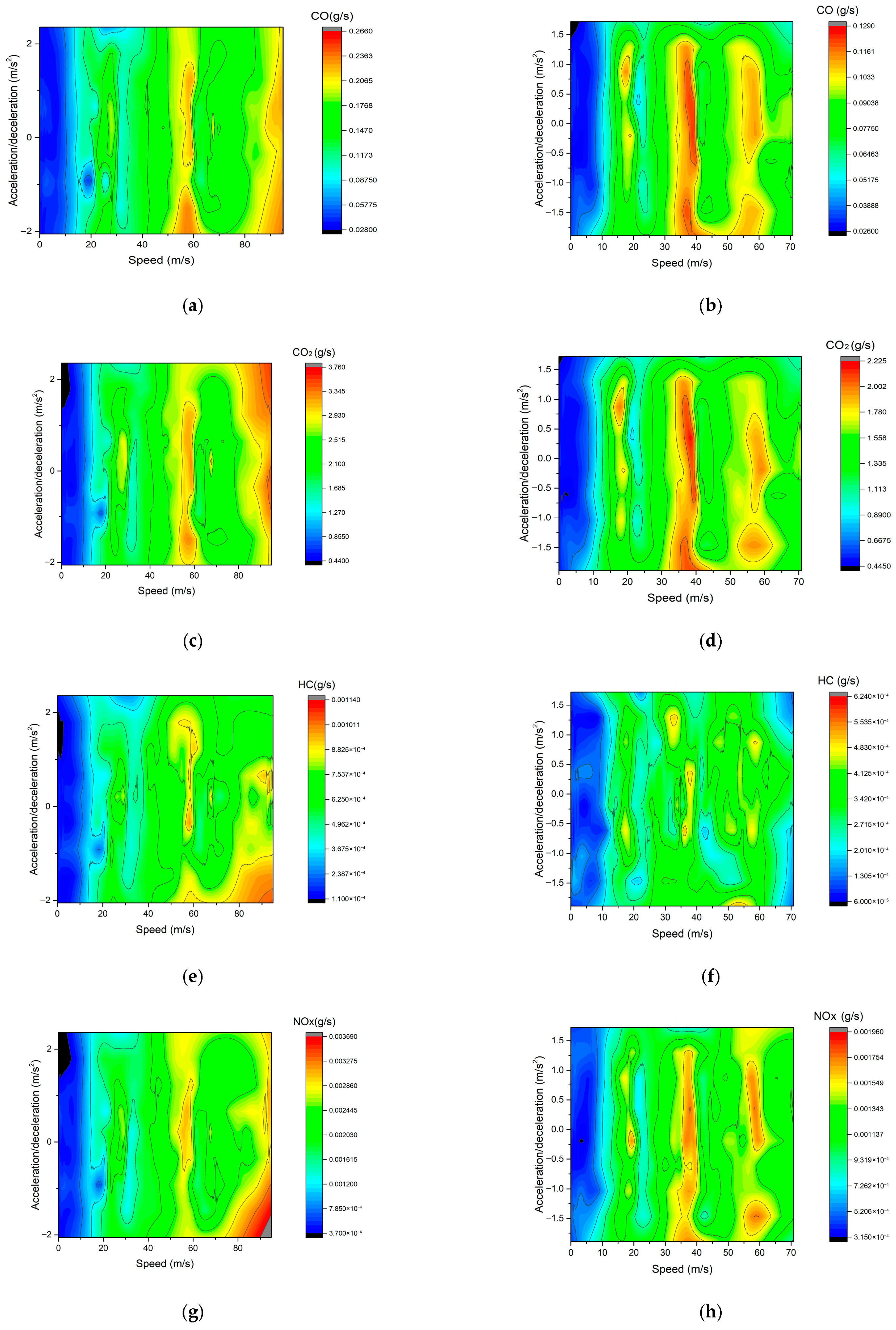
To compare the speed, acceleration/deceleration (A/D) behavior, and emission levels between the two driver types, contour plots were generated. Overall, CO and CO₂ exhaust emissions were consistently recorded at higher levels for aggressive drivers (Figure 6a,c) compared to non-aggressive drivers (Figure 6b,d). Moreover, the peak regions highlighted in Figure 6a–h correspond to conditions where exhaust emissions were markedly higher for aggressive drivers. This pattern can be attributed to their higher driving speeds, increased engine RPMs, and consequently greater exhaust flow rates Q_exhaust.

4.2. Comparison of RPM Considering A/D Behavior

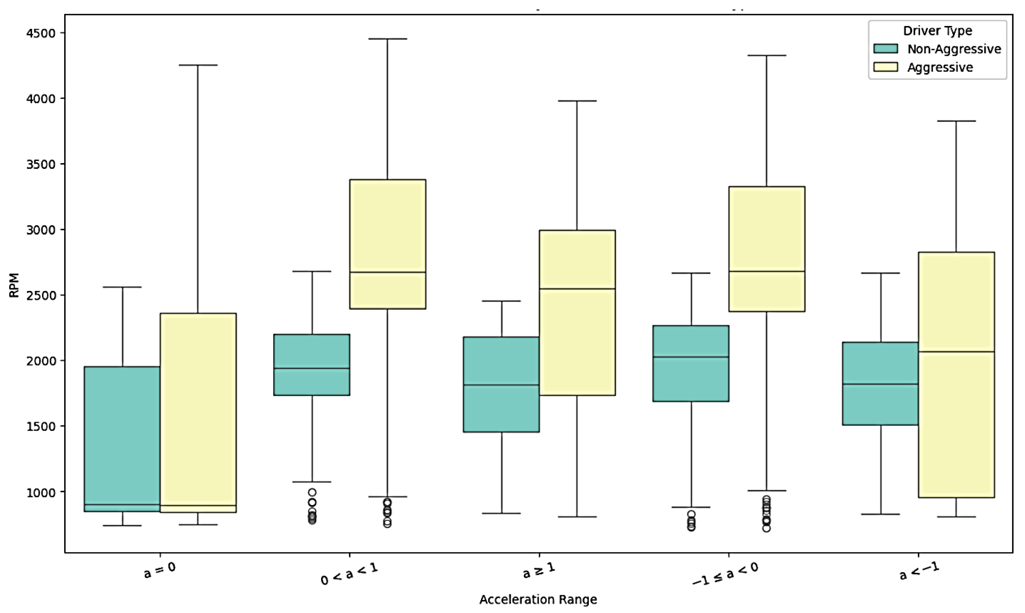
To compare engine RPM in relation to acceleration/deceleration (A/D) behavior between the two driver types, a box plot was used to illustrate the distribution of RPM across different A/D behaviors for both aggressive and non-aggressive drivers. As shown in Figure 7, aggressive drivers consistently exhibited higher RPM values compared to non-aggressive drivers across all A/D behavior categories. RPM analysis revealed that aggressive drivers consistently maintained higher engine RPMs across various acceleration and deceleration (A/D) phases, with an average RPM of 2302 compared to 1763 for non-aggressive drivers. To determine whether the differences in engine RPM between the two groups were statistically significant, a Mann–Whitney U test was conducted on the 920 RPM data points collected from each group’s 920-s driving cycle (

Table A8. Mann–Whitney U test results for comparing RPM between aggressive and non-aggressive drivers.

Test	Mann–Whitney U	Z	p-Value (2-Tailed)	Significant (α = 0.05)
Mann–Whitney U Test	665,992.5	21.4221	<0.001	Yes

in Appendix B). The results indicated that the RPM distributions for both aggressive and non-aggressive drivers significantly deviated from normality. The descriptive statistics further revealed that aggressive drivers had a higher sum of ranks than non-aggressive drivers. The Mann–Whitney U test confirmed that these differences were statistically significant (p < 0.05), demonstrating that aggressive drivers maintain significantly higher RPM levels compared to their non-aggressive counterparts.

4.3. Evaluation of the Effects of Driver Behavior on Emissions

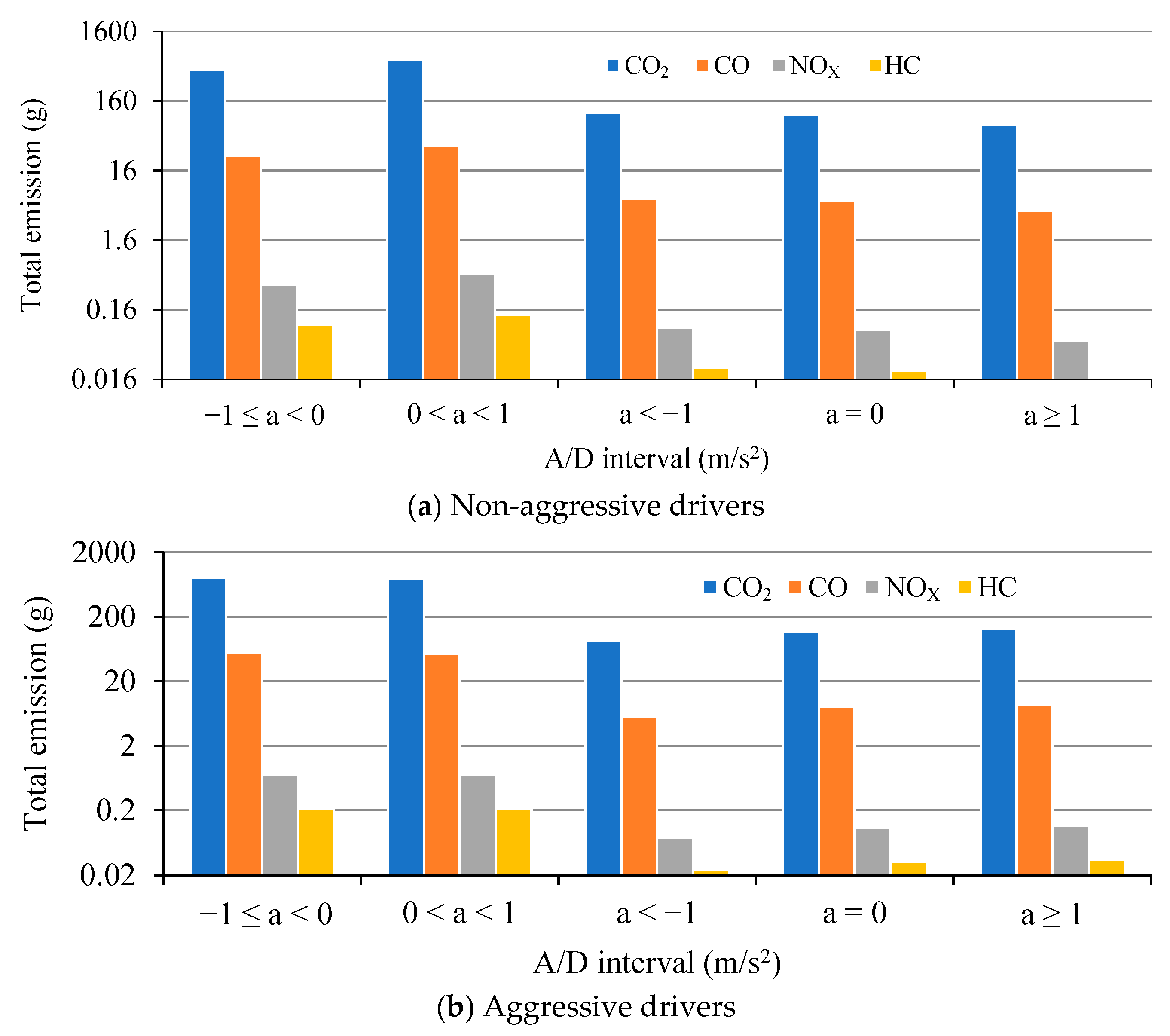
Tailpipe emissions of CO₂, CO, NO_X, and HC were measured continuously at one-second intervals throughout each group’s 920-s driving cycle. As illustrated in Figure 8, the instantaneous emission rates (g/s) were integrated over the full 920-s period to determine the total emissions (g) for each pollutant. The results in Figure 8 indicate that aggressive drivers consistently produced higher total tailpipe emissions of CO₂, CO, NO_X, and HC compared to non-aggressive drivers across all acceleration/deceleration (A/D) intervals. This pattern aligns with the higher engine RPMs and more abrupt driving behaviors typically observed among aggressive drivers. To identify the conditions under which most emissions occur, vehicle A/D behavior was divided into five intervals. The analysis revealed that the largest share of emissions was generated during mild acceleration and deceleration phases (−1 ≤ a < 0 and 0 < a < 1), as drivers spend the majority of their time operating within these intervals. In contrast, emissions were comparatively lower in other A/D intervals primarily because less time was spent in those ranges.

To evaluate uncertainty for vehicular emission predictions, two machine learning models, Random Forest (RF) and Gradient Boosting (GB), were employed, with their respective hyperparameters summarized in

Table 5. Hyperparameters for RF and GB algorithms.

Type of Driver	Parameter	Optimum Value
RF	n_estimators	500
	max_features	none
	min_samples_split	2
	min_samples_leaf	1
	Max_depth	10
GB	n_estimators	100
	min_samples_split	2
	Loss	Squared_error
	Learning rate	0.05
	Subsample	1
	Max_depth	3
	min_samples_split	2
	min_samples_leaf	1

Note. Random Forest (RF) and Gradient Boosting (GB).

. Both models were trained using 70% of the total dataset for training and validation, while the remaining 30% was reserved as the testing set. Model performance was assessed using Root Mean Squared Error (RMSE) and Mean Absolute Percentage Error (MAPE). As presented in

Table 6. RF and GB prediction performance.

Type of Driver	Emission	Model	RMSE	MAPE (%)
Aggressive driver	HC	Random Forest	0.0001	11.84
	HC	Gradient Boosting	0.0001	10.56
	NOX	Random Forest	0.0002	6.49
	NOX	Gradient Boosting	0.0001	6.46
	CO	Random Forest	0.0073	4.36
	CO	Gradient Boosting	0.0064	3.97
	CO2	Random Forest	0.1190	4.69
	CO2	Gradient Boosting	0.1067	4.47
Non-aggressive driver	HC	Random Forest	0.0001	23.47
	HC	Gradient Boosting	0.0001	23.13
	NOX	Random Forest	0.0001	8.88
	NOX	Gradient Boosting	0.0001	8.91
	CO	Random Forest	0.0037	3.34
	CO	Gradient Boosting	0.0033	3.12
	CO2	Random Forest	0.0749	4.30
	CO2	Gradient Boosting	0.0699	4.02

Note. Random Forest: RF; Gradient Boosting: Root Mean Squared Error: RMSE; Mean Absolute Percentage Error: MAPE; GB; CO: Carbon monoxide; CO₂: Carbon dioxide; HC: Hydrocarbon; NO_X: Nitrogen oxide.

, both metrics indicated low error values for aggressive and non-aggressive driver groups, reflecting high predictive accuracy of the models. Specifically, for aggressive drivers, the GB model achieved MAPE values as low as 3.97% for CO and 4.47% for CO₂, demonstrating excellent prediction performance. For HC and NO_X emissions, MAPE values for aggressive drivers ranged from 6.46% to 11.84%, indicating moderate yet acceptable error levels. Similarly, for non-aggressive drivers, both models maintained strong predictive accuracy; however, slightly higher errors were observed for HC predictions (MAPE ≈ 23%), while CO and CO₂ predictions remained highly accurate (MAPE ≈ 3–4%). Overall, the GB model slightly outperformed the RF model in most cases, particularly for CO and CO₂ emissions. These findings confirm that both RF and GB models provide reliable and accurate estimates of vehicular emissions with low uncertainty across the two driver behavior groups.

4.4. Correlation Analysis Between RPM and A/D Behavior on Tailpipe Emissions

The normality of RPM, A/D behavior, and the tailpipe emissions of the four main pollutants (CO₂, CO, NO_X, and HC) was assessed for datasets corresponding to non-aggressive and aggressive drivers using the Shapiro–Wilk test (

Table A9. Shapiro–Wilk test results for normality assessment of RPM distribution.

Driver Type	Shapiro–Wilk Statistic (W)	p-Value	Normal
Aggressive	0.9394	<0.001	No
Non-aggressive	0.934	<0.001	No

, Appendix B). These datasets were derived from the 920-s driving cycles for each driver group. According to the Shapiro–Wilk test results, all variables exhibited significant deviations from normality, indicating that the data were non-normally distributed. Due to this lack of normality, Spearman’s rank correlation analysis was employed to evaluate the relationships between RPM, A/D behavior, and the tailpipe emissions. The results are presented in

Table A10. Spearman correlation test results between RPM and tailpipe emissions.

Driver Type	Variable 1	Variable 2	Spearman	p-Value
Non-aggressive	RPM	CO2	0.788112	<0.0001
Non-aggressive	RPM	CO	0.741977	<0.0001
Non-aggressive	RPM	NOX	0.683403	<0.0001
Non-aggressive	RPM	HC	0.534305	<0.0001
Aggressive	RPM	CO2	0.702155	<0.0001
Aggressive	RPM	CO	0.736682	<0.0001
Aggressive	RPM	NOX	0.651359	<0.0001
Aggressive	RPM	HC	0.629091	<0.0001

Note. CO: Carbon monoxide; CO₂: Carbon dioxide; HC: Hydrocarbon; NO_X: Nitrogen oxide.

and

Table A11. Spearman correlation test results between A/D behavior and tailpipe emissions.

Driver Type	Variable 1	Variable 2	Spearman	p-Value
Non-aggressive	A/D	CO2	−0.00155	0.962676
Non-aggressive	A/D	CO	0.001542	0.962755
Non-aggressive	A/D	NOX	−0.00847	0.797634
Non-aggressive	A/D	HC	0.004454	0.576357
Aggressive	A/D	CO2	0.042715	0.196005
Aggressive	A/D	CO	0.038705	0.241383
Aggressive	A/D	NOX	0.059742	0.070413
Aggressive	A/D	HC	0.035003	0.068965

Note. Acceleration/deceleration (A/D); CO: Carbon monoxide; CO₂: Carbon dioxide; HC: Hydrocarbon; NO_X: Nitrogen oxide.

(Appendix B) for both driver groups. For non-aggressive drivers, the strongest positive correlation was observed between RPM and CO₂ tailpipe emissions (r = 0.788), while the weakest correlation was found between RPM and HC emissions (r = 0.534). In the aggressive driver group, the highest correlation occurred between RPM and CO emissions (r = 0.737), whereas the lowest correlation was again observed with HC emissions (r = 0.629). The relationship between A/D behavior and tailpipe emissions was also examined using Spearman’s rank correlation. Among non-aggressive drivers, the correlations between A/D behavior and all four pollutants were statistically insignificant. For example, the coefficients ranged from −0.008 (NO_X) to 0.004 (HC), with all p-values exceeding the significance threshold (p > 0.05). Similarly, in the aggressive driver group, the correlations between A/D behavior and emissions remained consistently weak. The highest observed correlation was between A/D variables and NO_X emissions (r = 0.059, p = 0.070), which was negligible. Other correlations were also non-significant. These findings indicate that, although A/D behavior is valuable for distinguishing driving styles, it does not demonstrate a meaningful relationship with tailpipe emission levels in either driver group. In contrast, RPM exhibits a strong and consistent correlation with emissions, highlighting its greater relevance as a predictor of vehicular pollutant output.

4.5. Estimation of Emission Factor Based on Driver Behavior

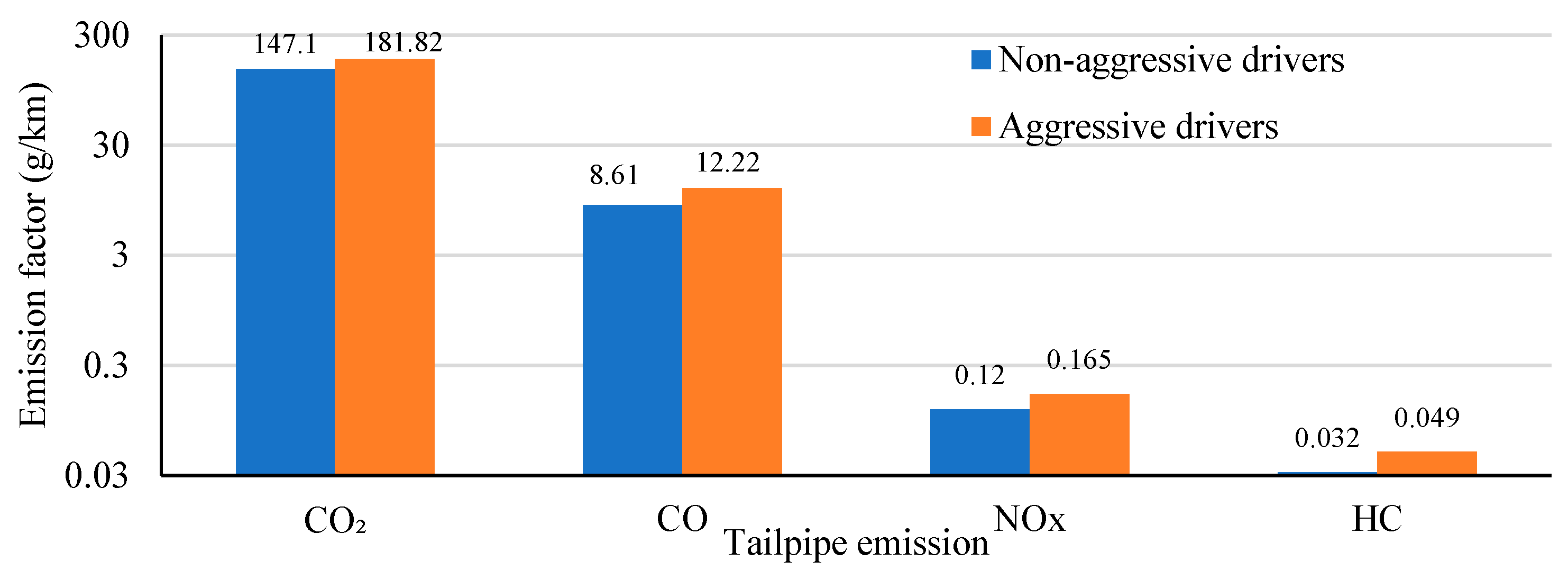
After calculating tailpipe emissions using Equations (1)–(4), the emission factors for each pollutant were determined using Equation (5) and are illustrated in Figure 9 for both aggressive and non-aggressive drivers. The results in Figure 9 reveal that the emission factor of CO₂ for aggressive drivers is approximately 23.6% higher than that of non-aggressive drivers. Similarly, the emission factor of CO is 41.9% higher in the aggressive driver group. For NO_X, the emission factor reached 0.165 g/km for aggressive drivers compared to 0.120 g/km for non-aggressive drivers, an increase of 37.5%. Moreover, the emission factor of HC was found to be 0.049 g/km in aggressive drivers, which is 53.13% higher than the value observed in the non-aggressive group (0.032 g/km). This comparative analysis clearly demonstrates that aggressive driving behavior is strongly associated with elevated emission factors across all major pollutants, underscoring the critical role of driver behavior in influencing vehicular emissions.

4.6. Comparison of the Results with Those of Other Studies

The results of the present study, obtained using on-board measurements, reveal that the emission factors of NO_X, CO₂, CO, and HC for aggressive drivers were 37.50%, 23.60%, 41.90%, and 53.13% higher, respectively, than those for non-aggressive drivers. These findings are consistent with Chandrashekar et al. [39], who reported that aggressive driving increased the emission factors of CO, HC, and CO₂ by 5–25% compared to normal driving on both urban and rural roads. Our results thus corroborate the conclusion that aggressive driving behavior elevates emission factors across all major pollutants. A comparison of the emission factors obtained in this study with those reported by Pouresmaeili et al. [55] underscores the significant influence of road type on vehicular emissions. In the present study, which focused on urban highways, the measured emission factors of aggressive drivers for CO₂, CO, NO_X, and HC were 181.82, 12.22, 0.165, and 0.049 g/km, respectively. In contrast, Pouresmaeili et al. [55], who examined urban roads with frequent stop-and-go traffic and signalized intersections, reported substantially higher values: 392, 945, 2.05, and 0.06 g/km, respectively. These discrepancies highlight that highways, characterized by more continuous driving and fewer acceleration/deceleration (A/D) events, tend to generate lower emissions than congested urban roads. The strong positive Spearman correlations observed in this study between engine speed (RPM) and emissions, ranging from 0.53–0.79 for non-aggressive drivers and 0.63–0.74 for aggressive drivers, further emphasize the role of engine dynamics in pollutant output. This result aligns with the findings of Zhai et al. [56], who also reported significant correlations between emissions (CO₂, CO, and NO_X) and engine parameters. Moreover, the observation that aggressive drivers consistently emitted higher levels of pollutants corroborates the conclusions of Zheng et al. [20], who demonstrated that aggressive driving leads to significantly elevated emission levels compared with non-aggressive driving.

To benchmark these results against international emission standards, the study compared the calculated emission factors with the Euro 4 standard [57] (

Table 7. Comparison of emission factor via Euro 4 standard.

Driving Style	CO (g/km)	NOX (g/km)	HC (g/km)	CO2 (g/km)
Non-aggressive driver	8.61	0.12	0.032	147.10
aggressive Driver	12.22	0.165	0.049	181.82
Euro 4 Standard	1.0	0.08	0.10	N/A

Note. CO: Carbon monoxide; CO₂: Carbon dioxide; HC: Hydrocarbon; NO_X: Nitrogen oxide; N/A: Not available.

). For non-aggressive drivers, the emission factors of CO, NO_X, and HC were 8.61, 0.12, and 0.032 g/km, respectively, whereas for aggressive drivers, these values increased to 12.22, 0.165, and 0.049 g/km. When compared with the Euro 4 limits of 1.0 g/km for CO, 0.08 g/km for NO_X, and 0.10 g/km for HC, it becomes evident that real-world CO and NO_X emissions particularly under aggressive driving conditions far exceed regulatory thresholds. Conversely, HC emissions remained below the Euro 4 limit. The Euro 4 standard does not specify a threshold for CO₂, limiting direct comparisons for this pollutant. These findings highlight that driving behavior has a profound impact on actual on-road emissions. Even vehicles that are compliant with Euro 4 regulations under laboratory conditions can produce several-fold higher emissions in real-world driving, especially for CO. This underscores the need to account for real-world driving conditions when assessing vehicular emissions and their impact on urban air quality, particularly within the Iranian driver population.

4.7. Limitations of the Study and Suggestions for Future Research

This study investigated the impact of driver behavior classified as aggressive and non-aggressive on tailpipe emissions and proposed emission factors specific to urban highways. However, several limitations should be acknowledged. First, the analysis focused exclusively on urban highways, while arterial roads with more complex traffic conditions, intersections, and stop-and-go patterns were not examined. Second, the influence of seasonal variation on tailpipe emissions and the effects of environmental factors such as diverse weather conditions (e.g., temperature extremes, humidity fluctuations, or precipitation) were not comprehensively addressed. Future research should aim to broaden the sample size and include multiple road types including arterial roads, rural roads, and urban streets to better capture the variability in driving conditions. Incorporating seasonal factors and a wider range of vehicle types and engine characteristics would also allow for a more holistic understanding of the relationship between driver behavior and emissions. In addition, employing advanced modeling approaches such as deep neural networks or reinforcement learning algorithms could enhance the ability to analyze complex driving behaviors and predict emissions under diverse road conditions, seasons, and vehicle types. Furthermore, integrating driving behavior data with traffic parameters and environmental variables could lead to the development of more accurate, robust, and practical emission prediction models that better reflect real-world scenarios.

5. Conclusions

On urban highways, driver behavior plays a crucial role in influencing tailpipe emissions. Given the adverse impacts of vehicular pollutants on air quality and public health, it is essential to monitor and control these emissions within air pollution models that account for driver behavior. This objective can be achieved by estimating the emission factors of key pollutants, namely CO, CO₂, NO_X, and HC, with respect to the behavioral characteristics of different driver types. To propose emission factors for air pollution models that incorporate driver behavior on urban highways, the present study focused on urban highways in Mashhad, Iran. Driver behavior was first assessed using the Driver Behavior Questionnaire (DBQ), and drivers were subsequently classified into aggressive and non-aggressive groups using the K-means clustering algorithm based on four key parameters: the average DBQ score, maximum acceleration, the number of maximum acceleration events, and the number of traffic accidents recorded over five years. Finally, the impact of driver behavior on emission factors was evaluated using an on-board measurement method to capture real-world emission data. The most significant findings of this research are summarized as follows:

• After clustering 150 drivers based on four key parameters and selecting 10 representative drivers from each group, driving cycles were developed for both aggressive and non-aggressive drivers. The results showed that the average speed for aggressive drivers (40.54 km/h) was higher than that of non-aggressive drivers (34.27 km/h), indicating that aggressive drivers tend to maintain higher driving speeds. The maximum speeds further emphasized this distinction, with aggressive drivers reaching 91 km/h, while non-aggressive drivers peaked at 70 km/h. Similarly, the mean positive acceleration was greater for aggressive drivers (0.53 m/s²) compared to non-aggressive drivers (0.45 m/s²), reflecting their tendency toward more rapid acceleration. These differences in speed and acceleration clearly highlight the distinctive driving characteristics of aggressive drivers.
• RPM analysis revealed that aggressive drivers consistently maintained higher engine RPMs across various acceleration and deceleration (A/D) phases, with an average RPM of 2302 compared to 1763 for non-aggressive drivers. To statistically evaluate these differences, the Mann–Whitney U test was conducted, which confirmed significant differences in tailpipe emissions between the two driver groups. This finding demonstrates that aggressive driving behavior contributes to substantially higher emissions.
• The study further revealed that engine RPM plays a significant role in increasing the concentrations of the four main pollutants (CO₂, CO, NO_X, and HC), whereas A/D behavior showed no meaningful direct impact on emission levels. Nevertheless, A/D behavior proved to be a useful parameter for distinguishing driving styles, despite its weak correlation with pollutant emissions. These findings suggest that strategies to reduce vehicular pollution should prioritize RPM control while still considering A/D patterns to identify high-emission driving behaviors.
• Results obtained using the on-board measurement method showed that the emission factors of NO_X, CO₂, CO, and HC for aggressive drivers were 37.50%, 23.60%, 41.90%, and 53.13% higher, respectively, than those of non-aggressive drivers. These findings highlight that driving behavior directly influences vehicular emissions, and the differences between the clusters were clearly reflected in their emission factors.

References

1. World Health Organization (WHO). Ambient Air Pollution: A Global Assessment of Exposure and Burden of Disease. 2016. Available online: https://www.who.int/publications/i/item/9789241511353 (accessed on 1 December 2022).
2. Aminzadegan, S.; Shahriari, M.; Mehranfar, F.; Abramović, B. Factors affecting the emission of pollutants in different types of transportation: A literature review. Energy Rep. 2022, 8, 2508–2529. [Google Scholar] [CrossRef]
3. Raparthi, N.; Barudgar, A.; Chu, M.; Ning, Z.; Phuleria, H.C. Estimating individual vehicle emission factors from near-road measurements in India. Atmos. Environ. 2023, 308, 119869. [Google Scholar] [CrossRef]
4. World Bank. Total Greenhouse Gas Emissions (kt of CO2 Equivalent)—Iran. Islamic Rep, World Bank. 2022. Available online: https://data.worldbank.org/indicator/EN.ATM.GHGT.KT.CE?locations=IR&most_recent_value_desc=true (accessed on 4 March 2023).
5. In-Service Conformity (ISC). The Contribution of the Transportation Sector in the Emission of Pollutants and Greenhouse Gases in Iran. 2020. Available online: https://amar.org.ir/statistical-information/statid/21923 (accessed on 7 June 2025).
6. Shahbazi, H.; Reyhanian, M.; Hosseini, V.; Afshin, H. The relative contributions of mobile sources to air pollutant emissions in Tehran, Iran: An emission inventory approach. Emiss. Control Sci. Technol. 2016, 2, 44–56. [Google Scholar] [CrossRef]
7. Iranian Labour News Agency (ILNA). 2022. Available online: https://www.ilna.ir/fa/tiny/news-1317914 (accessed on 21 July 2023).
8. Demir, A. Investigation of air quality in the underground and aboveground multi-storey car parks in terms of exhaust emissions. Procedia-Soc. Behav. Sci. 2015, 195, 2601–2611. [Google Scholar] [CrossRef]
9. Fontaras, G.; Zacharof, N.G.; Ciuffo, B. Fuel consumption and CO2 emissions from passenger cars in Europe–Laboratory versus real-world emissions. Prog. Energy Combust. Sci. 2017, 60, 97–131. [Google Scholar] [CrossRef]
10. Pirayre, A.; Michel, P.; Rodriguez, S.S.; Chasse, A. Driving behavior identification and real-world fuel consumption estimation with crowdsensing data. IEEE Trans. Intell. Transp. Syst. 2022, 23, 18378–18391. [Google Scholar] [CrossRef]
11. Singh, H.; Kathuria, A. Analyzing driver behavior under naturalistic driving conditions: A review. Accid. Anal. Prev. 2021, 150, 105908. [Google Scholar] [CrossRef]
12. Hadadi, F.; Tehrani, H.G.; Aghayan, I. An extended non-lane-discipline-based continuum model through driver behaviors for analyzing multi-traffic flows. Phys. A Stat. Mech. Its Appl. 2023, 625, 128965. [Google Scholar] [CrossRef]
13. Munigety, C.R.; Mathew, T.V. Towards behavioral modeling of drivers in mixed traffic conditions. Transp. Dev. Econ. 2016, 2, 1–20. [Google Scholar] [CrossRef]
14. Rezaei, D.; Aghayan, I.; Hadadi, F. Studying perturbations and wave propagations by lane closures on traffic characteristics based on a dynamic approach. Phys. A Stat. Mech. Its Appl. 2021, 566, 125654. [Google Scholar] [CrossRef]
15. Lu, M. Comparison of driver classification based on subjective evaluation and objective experiment. In Proceedings of the 90th TRB Annual Meeting, Washington, DC, USA, 23–27 January 2011. No. 11-3170. [Google Scholar]
16. Li, P.; Shi, J.; Liu, X. Driving style recognition based on driver behavior questionnaire. Open J. Appl. Sci. 2017, 7, 115–128. [Google Scholar] [CrossRef]
17. Gupta, L.; Goswami, S.; Kumar, R. Analysis of driver behaviours towards road safety measures using DBQ in the Indian context. Trans. Transp. Sci. 2021, 12, 12–18. [Google Scholar] [CrossRef]
18. Youssef, D.; Salameh, P.; Abou-Abbas, L.; Salmi, L.R. Examining self-reported aberrant behavior among Lebanese drivers using the Driver Behavior Questionnaire (DBQ). Discov. Soc. Sci. Health 2023, 3, 25. [Google Scholar]
19. Eboli, L.; Mazzulla, G.; Pungillo, G. Combining speed and acceleration to define car users’ safe or unsafe driving behaviour. Transp. Res. Part. C Emerg. Technol. 2016, 68, 113–125. [Google Scholar] [CrossRef]
20. Zheng, F.; Li, J.; Van Zuylen, H.; Lu, C. Influence of driver characteristics on emissions and fuel consumption. Transp. Res. Procedia 2017, 27, 624–631. [Google Scholar] [CrossRef]
21. Ma, Y.; Tang, K.; Chen, S.; Khattak, A.J.; Pan, Y. On-line aggressive driving identification based on in-vehicle kinematic parameters under naturalistic driving conditions. Transp. Res. Part C Emerg. Technol. 2020, 114, 554–571. [Google Scholar] [CrossRef]
22. Ameen, H.A.; Mahamad, A.K.; Saon, S.; Malik, R.Q.; Kareem, Z.H.; Bin Ahmadon, M.A.; Yamaguchi, S. Identification of driving safety profiles in vehicle-to-vehicle communication system based on vehicle OBD information. Information 2021, 12, 194. [Google Scholar] [CrossRef]
23. Liu, Z.; Chen, H.; Li, Y.; Zhang, Q. Taxi demand prediction based on a combination forecasting model in hotspots. J. Adv. Transp. 2020, 2020, 1302586. [Google Scholar] [CrossRef]
24. Liu, Z.; Chen, H. Short-term online taxi-hailing demand prediction based on the multimode traffic data in metro station areas. J. Transp. Eng. Part A Syst. 2022, 148, 05022003. [Google Scholar] [CrossRef]
25. Jung, H. A Comparison of Driving Characteristics and Environmental Characteristics Using Factor Analysis and K-Means Clustering Algorithm. Ph.D. Thesis, Virginia Polytechnic Institute and State University, Blacksburg, VA, USA, 2012. [Google Scholar]
26. Serttaş, T.N.; Gerek, Ö.N.; Hocaoğlu, F.O. Driver classification using K-means clustering of within-car accelerometer data. In Proceedings of the 2019 27th Signal Processing and Communications Applications Conference (SIU), Sivas, Turkey, 24–26 April 2019; IEEE: New York, NY, USA, 2019; pp. 1–4. [Google Scholar]
27. Adamidis, F.K.; Mantouka, E.G.; Vlahogianni, E.I. Effects of controlling aggressive driving behavior on network-wide traffic flow and emissions. Int. J. Transp. Sci. Technol. 2020, 9, 263–276. [Google Scholar] [CrossRef]
28. Mohammadnazar, A.; Khattak, Z.H.; Khattak, A.J. Assessing driving behavior influence on fuel efficiency using machine-learning and drive-cycle simulations. Transp. Res. Part D Transp. Environ. 2024, 126, 104025. [Google Scholar] [CrossRef]
29. Du, X.; Kang, X.; Gao, Y.; Wang, X. Driving behavior characterization and traffic emission analysis considering the vehicle trajectory. Front. Psychol. 2024, 14, 1341611. [Google Scholar] [CrossRef]
30. Almachi, J.C.; Saguay, J.; Anrango, E.; Cando, E.; Reina, S. Clustering-Based Urban Driving Cycle Generation: A Data-Driven Approach for Traffic Analysis and Sustainable Mobility Applications in Ecuador. Sustainability 2025, 17, 3353. [Google Scholar] [CrossRef]
31. Nam, E.K.; Gierczak, C.A.; Butler, J.W. A comparison of real-world and modeled emissions under conditions of variable driver aggressiveness. In Proceedings of the 82nd Annual Meeting of the Transportation Research Board, Washington, DC, USA, 12–16 January 2003. [Google Scholar]
32. Nesamani, K.S. Estimation of automobile emissions and control strategies in India. Sci. Total Environ. 2010, 408, 1800–1811. [Google Scholar] [CrossRef]
33. McGordon, A.; Poxon, J.E.; Cheng, C.; Jones, R.P.; Jennings, P.A. Development of a driver model to study the effects of real-world driver behaviour on the fuel consumption. Proc. Inst. Mech. Eng. Part D J. Automob. Eng. 2011, 225, 1518–1530. [Google Scholar] [CrossRef]
34. Yao, Y.; Zhao, X.; Liu, C.; Rong, J.; Zhang, Y.; Dong, Z.; Su, Y. Vehicle fuel consumption prediction method based on driving behavior data collected from smartphones. J. Adv. Transp. 2020, 2020, 9263605. [Google Scholar] [CrossRef]
35. Carrese, S.; Gemma, A.; La Spada, S. Impacts of driving behaviours, slope and vehicle load factor on bus fuel consumption and emissions: A real case study in the city of Rome. Procedia-Soc. Behav. Sci. 2013, 87, 211–221. [Google Scholar] [CrossRef]
36. Zheng, F.; Li, J.; Van Zuylen, H.J.; Lu, C. Influence of driver characteristics on emissions and fuel consumption. IET Intell. Transp. Syst. 2019, 13, 1770–1779. [Google Scholar] [CrossRef]
37. Huang, Y.; Ng, E.C.; Zhou, J.L.; Surawski, N.C.; Lu, X.; Du, B.; Forehead, H.; Perez, P.; Chan, E.F. Impact of drivers on real-driving fuel consumption and emissions performance. Sci. Total Environ. 2021, 798, 149297. [Google Scholar] [CrossRef]
38. Suarez, J.; Makridis, M.; Anesiadou, A.; Komnos, D.; Ciuffo, B.; Fontaras, G. Benchmarking the driver acceleration impact on vehicle energy consumption and CO2 emissions. Transp. Res. Part D Transp. Environ. 2022, 107, 103282. [Google Scholar] [CrossRef]
39. Chandrashekar, C.; Rawat, R.S.; Chatterjee, P.; Pawar, D.S. Evaluating the real-world emissions of diesel passenger Car in Indian heterogeneous traffic. Environ. Monit. Assess. 2023, 195, 1248. [Google Scholar] [CrossRef]
40. Jia, Z.; Yin, J.; Cao, Z.; Wei, N.; Jiang, Z.; Zhang, Y.; Wu, L.; Zhang, Q.; Mao, H. Sustainable transportation emission reduction through intelligent transportation systems: Mitigation drivers, and temporal trends. Environ. Impact Assess. Rev. 2025, 112, 107767. [Google Scholar] [CrossRef]
41. Planning and Development Department of the Municipality of Mashhad. Statistical Yearbook of Mashhad; Planning and Development Department of the Municipality of Mashhad: Mashhad, Iran, 2025. Available online: https://planning.mashhad.ir/s/mfaPNuZ (accessed on 7 May 2025).
42. Sadeghi, M. Transport Sustainability Study: Mashhad, Islamic Republic of Iran; ESCAP Publications: Bangkok, Thailand, 2021. [Google Scholar]
43. Vakili, V.; Zarifian, A.R.; Khadem-Rezaiyan, M. Predictors of public transportation in Mashhad: A population-based study. J. Educ. Health Promot. 2018, 7, 5. [Google Scholar]
44. CTPM. Authority Report of Public Transportation System in Transportation Plan of Mashhad; Urban Traffic Organization in Mashhad Municipality: Mashhad, Iran, 2015. (In Persian) [Google Scholar]
45. AVL Di TEST MDS User Manual. Available online: https://www.avlditest.com/en/downloads-en.html (accessed on 15 June 2022).
46. Likert, R. A technique for the measurement of attitudes. Arch. Psychol. 1932, 22, 1–55. [Google Scholar]
47. Parishad, N.; Aghabayk, K.; Rezaie, R.; Samerei, A.; Mohammadi, A. Validation of the driver behavior questionnaire in a representative sample of Iranian drivers. Civ. Eng. Infrastruct. J. 2020, 53, 161–171. [Google Scholar]
48. Cronbach, L.J. Coefficient alpha and the internal structure of tests. Psychometrika 1951, 16, 297–334. [Google Scholar] [CrossRef]
49. Banerjee, A.; Dave, R.N. Validating clusters using the Hopkins statistic. In Proceedings of the 2004 IEEE International Conference on Fuzzy Systems (IEEE Cat. No. 04CH37542), Budapest, Hungary, 25–29 July 2004; IEEE: New York, NY, USA, 2004; Volume 1, pp. 149–153. [Google Scholar]
50. Dalmaijer, E.S.; Nord, C.L.; Astle, D.E. Statistical power for cluster analysis. BMC Bioinform. 2022, 23, 205. [Google Scholar] [CrossRef]
51. Yan, G.; Wang, M.; Qin, P.; Yan, T.; Li, K.; Wang, X.; Han, C. Field measurements of vehicle pollutant emissions in road tunnels at different altitudes. Tunn. Undergr. Space Technol. 2021, 118, 104187. [Google Scholar] [CrossRef]
52. Welstand, J.S.; Haskew, H.H.; Gunst, R.F.; Bevilacqua, O.M. Evaluation of the effects of air conditioning operation and associated environmental conditions on vehicle emissions and fuel economy. SAE Trans. 2003, 112, 1993–2006. [Google Scholar]
53. De Vlieger, I. On board emission and fuel consumption measurement campaign on petrol-driven passenger cars. Atmos. Environ. 1997, 31, 3753–3761. [Google Scholar] [CrossRef]
54. Lents, J.; Davis, N. International Vehicle Emission (IVE) Model Users Manual; Technical Report; International Sustainable Systems Research Center: La Habra, CA, USA, 2004. [Google Scholar]
55. Pouresmaeili, M.A.; Aghayan, I.; Taghizadeh, S.A. Development of Mashhad driving cycle for passenger car to model vehicle exhaust emissions calibrated using on-board measurements. Sustain. Cities Soc. 2018, 36, 12–20. [Google Scholar] [CrossRef]
56. Zhai, Z.; Tu, R.; Xu, J.; Wang, A.; Hatzopoulou, M. Capturing the variability in instantaneous vehicle emissions based on field test data. Atmosphere 2020, 11, 765. [Google Scholar] [CrossRef]
57. Emission Standards. Euro 4 Standard. Available online: https://dieselnet.com/standards/eu/ld.php?utm_source=chatgpt.com#stds/standards/eu/ld.php?utm_source=chatgpt.com#stds (accessed on 3 October 2025).
Figure 1. Flow chart of the present study.
Eng 06 00294 g001
Figure 2. Geographical location of the studied highways (maps from Google Earth®). Note. Rectangular shapes over the map show the studied sections.
Eng 06 00294 g002
Figure 3. Determination of the number of clusters using the silhouette coefficient.
Eng 06 00294 g003
Figure 4. Exhaust flow rate based on RPM. Note. RPM: Revolutions per minute.
Eng 06 00294 g004
Figure 5. Driving cycle of aggressive and non-aggressive drivers on urban highways.
Eng 06 00294 g005
Figure 6. The relationship between the effects of speed and A/D behavior on CO, CO2, HC, and NOX tailpipe emission for aggressive and non-aggressive drivers. (a) The relationship between the effect of speed and A/D on CO for aggressive drivers. (b) The relationship between the effect of speed and A/D on CO for non-aggressive drivers. (c) The relationship between the effect of speed and A/D on CO2 for aggressive drivers. (d) The relationship between the effect of speed and A/D on CO2 for non-aggressive drivers. (e) The relationship between the effect of speed and A/D on HC for aggressive drivers. (f) The relationship between the effect of speed and A/D on HC for non-aggressive drivers. (g) The relationship between the effect of speed and A/D on NOX for aggressive driver. (h) The relationship between the effect of speed and A/D on NOX for non-aggressive driver. Note. Acceleration/deceleration (A/D); CO: Carbon monoxide; CO2: Carbon dioxide; HC: Hydrocarbon; NOX: Nitrogen oxide.
Eng 06 00294 g006
Figure 7. Box plot of RPM during different A/D behaviors for aggressive and non-aggressive drivers.
Eng 06 00294 g007
Figure 8. Tailpipe emissions across different A/D ranges. Note. Acceleration/deceleration (A/D); CO: Carbon monoxide; CO2: Carbon dioxide; HC: Hydrocarbon; NOX: Nitrogen oxide.
Eng 06 00294 g008
Figure 9. Comparison of emission factors of four main pollutants. Note. CO: Carbon monoxide; CO2: Carbon dioxide; HC: Hydrocarbon; NOX: Nitrogen oxide.
Eng 06 00294 g009