Article

Probabilistic Estimation of Parameters for Lubrication Application with Neural Networks

by
Stefan Paschek
1,*,
Frederic Förster
2,
Martin Kipfmüller
3,* and
Michael Heizmann
4
1
Department Electronic Engineering, UAS Fachhochschule Technikum Wien, 1200 Vienna, Austria
2
Walther Systemtechnik GmbH, 76726 Germersheim, Germany
3
Institute of Materials and Processes, UAS Hochschule Karlsruhe, 76012 Karlsruhe, Germany
4
Institute of Industrial Information Technologies, KIT Karlsruher Institut für Technologie, 76131 Karlsruhe, Germany
*
Authors to whom correspondence should be addressed.
Eng 2024, 5(4), 2428-2440; https://doi.org/10.3390/eng5040127
Submission received: 5 July 2024 / Revised: 18 September 2024 / Accepted: 20 September 2024 / Published: 30 September 2024

Abstract

:
This paper investigates the use of neural networks to predict characteristic parameters of the grease application process pressure curve. A combination of two feed-forward neural networks was used to estimate both the value and the standard deviation of selected features. Several neuron configurations were tested and evaluated in their capability to make a probabilistic estimation of the lubricant’s parameters. The value network was trained with a dataset containing the full set of features and with a dataset containing its average values. As expected, the full network was able to predict noisy features well, while the average network made smoother predictions. This is also represented by the networks’ R2 values which are 0.781 for the full network and 0.737 for the mean network. Several further neuron configurations were tested to find the smallest possible configuration. The analysis showed that three or more neurons deliver the best fit over all features, while one or two neurons are not sufficient for prediction. The results showed that the grease application process pressure curve via pressure valves can be estimated by using neural networks.

1. Introduction

In modern products, grease has many different areas of application, ranging from the traditional prevention of wear and tear to modifying the haptic properties of the product by changing the frictions and therefore varying the force required to press buttons or the torque required to turn rotary knobs. Recent advances in the field of tribology focus on green concepts such as polyvinyl alcohol (PVA) instead of traditional petroleum-based solutions. Here, in particular, [1] and a previous study [2] show promising results.
The focus of this paper is on the application process of grease as lubricant. To be specific, the pulsing ejaculation of grease using pressure valves. Grease application processes are highly dependent on parameters such as temperature and material pressure. As grease is compressible, its behavior also changes depending on how long it is exposed to pressure. Furthermore, the very rough classification based on NLGI classes (see [3]) introduces additional uncertainty into the process. Based on the rough classification, grease producers can change their recipes without leaving the boundaries of their respective NLGI class but with strong influences on the behavior of the grease. In addition, even parameters such as storage time and the grease’s mass might influence it, as its own weight can lead to a separation of fat and binder, which can affect the grease’s viscosity. All of these issues create uncertainty in predicting the results and behavior of the grease during the application processes. The pressure curve of the grease might vary, which in turn will affect the weight and shape of the ejected grease pulse. During the application process, the grease pressure curve within the valve is one of the main influences on the applied grease mass and shape. The pressure curve includes all application parameters, such as grease state, temperature, valve parameters, and so on. When the valve opens and allows grease to be ejaculated outwards during a pulsing action, the pressure within the valve drops rapidly. This pressure curve is measured and used for analysis. As the pressure curve can also vary greatly depending on the lubricant parameters, it is difficult to decide whether the curve varies due to external disturbances or whether the whole grease has changed its characteristics due to separation of fat and binder. Therefore, this paper describes a probabilistic neural network approach to create a pressure prediction that includes a confidence interval. This confidence interval is used to predict the parameter behavior of the pressure curve and to estimate whether the grease has changed its internal parameters. The focus of this paper will be whether a neural network can be used to predict such features both in their expected value and their standard deviation.
One way of predicting features and their statistical properties is to use probabilistic neural networks, which were introduced in 1988 [4] as an additional solution for pattern classification problems. Since their introduction, feed-forward networks have been successfully used for regression of features in medical fields such as in [5]. Here, the advantages of fast training, the ability to deal with changing data, and a possible confidence statement that provides an estimate of correctness come into play. One of the most important advantages is that training is easy and instantaneous (see [6]). For this reason, probabilistic neural networks are used, for example, in tumor detection, since the network provides fast and accurate classification (see [7]).

Problem Description

The aim of the research projects is to develop a methodology to create a predictive model for the grease application process. The main parameters of interest are grease mass and shape after application. In future work, an adaptive intelligent control algorithm will be developed to compensate for internal and external disturbances. During the grease application process, its pressure follows a characteristic curve. The shape of this curve is one of the most important influences on the quality of the process. Even if external influences such as temperature are measured, the pressure curve itself is additionally influenced by the compressibility and varying viscosity of the grease. In practice grease application experts often set the necessary process parameters based on their experience. The prediction of pressure curve parameters can give these experts additional information to improve the setup process and save time for calibrating the valve parameters. This paper focuses on the first step in achieving the project objectives, the creation of a neural network to predict the main parameters of the pressure curve and their variances.

2. Materials and Methods

2.1. Test Stand and Methodology

In order to generate sufficient samples for statistical analysis of the pressure curves and all influencing parameters, an automated test rig had to be set up. Figure 1 shows the basic setup with the main components. The test stand contains a buffer storage for plastic plates, which are used as specimens. An industrial robotic arm with vacuum gripping technology is used to move the specimen. An MPP03Pro pulse valve is used to ejaculate grease in pulsing mode onto the specimen. A pressure sensor is used to measure the pressure flow during the application process. A high-precision scale is used to measure the grease mass after application. A camera is used to analyze the shape of the grease.
Every application consists of the following steps:
  • Robot picks up specimen from buffer storage.
  • Robot places specimen on scale to measure empty weight.
  • Robot moves specimen to pulsing valve position.
    a.
    Pulsing valve shoots 15 single grease points onto the specimen.
    b.
    Robot moves after every shot to prevent overlapping.
  • Robot places specimen on scale to measure full weight.
  • Robot moves specimen to camera station.
    a.
    Picture from front view is taken.
    b.
    Picture from side view is taken.
  • Robot places specimen on exit station.
  • Back to nr. 1.
A total of 8760 measurements were taken using this semi-automated test stand setup. These measurements were used to model pressure curve parameters.

2.2. Grease Application Process

The grease application process consists of three components. The first component is a pneumatic pump. This pump presses down on a grease-filled container at a pressure of 50 bar. The pressure causes the grease to turn into a non-Newtonian liquid. The liquefied grease is then passed through the second component, a grease pressure regulator. This pressure controller is used to regulate the pressure of the liquid to a set point. At the outlet of the pressure controller’s output, the grease flows into the third component, a pulsing valve. The pulsing valve contains a heater and a pressure sensor. The pulsing valve releases the grease after a pneumatically controlled pin is moved by a pressure of 8 bar. The pin can be tensioned by a tension spring using a knob. When the pin is released, grease can flow out of the valve opening. When the pin is closed, the material stops flowing. Typical opening times vary from 4 ms to 20 ms. The result of a grease application is shown in Figure 2.
The pressure valve has four main control parameters that influence the application behavior of the grease:
  • Pressure set point on the pressure controller.
  • Temperature set point on the temperature controller.
  • Pin tension.
  • Valve pin release time (opening time of valve).
These parameters are normalized and used as inputs to the probabilistic neural pressure prediction model. As the initial pressure of the grease application process within the valve is highly dependent on the compression time, the initial pressure will also be used as an input parameter. The main output parameters for this model will be the pressure curve features described in the next section.

2.3. Pressure Curve

The pressure curves of grease application processes follow a characteristic shape as shown in Figure 3. In addition to the four valve control variables mentioned in Section 2.2, there are other variables that influence the pressure curve behavior. For example, even when using the same type of grease from the same manufacturer, the viscosity can vary greatly within an NLGI class. Temperature can also have a significant effect on grease viscosity. Unfortunately, grease can also change its system behavior depending on storage time and storage weight. The so called “oil bleeding” effect can cause a separation of grease and oil based on high and continuous pressure, which in turn can cause areas of varying viscosity in stored grease (see [8,9] for a deeper explanation). Therefore, these factors can also influence the curve but were not considered in this paper.
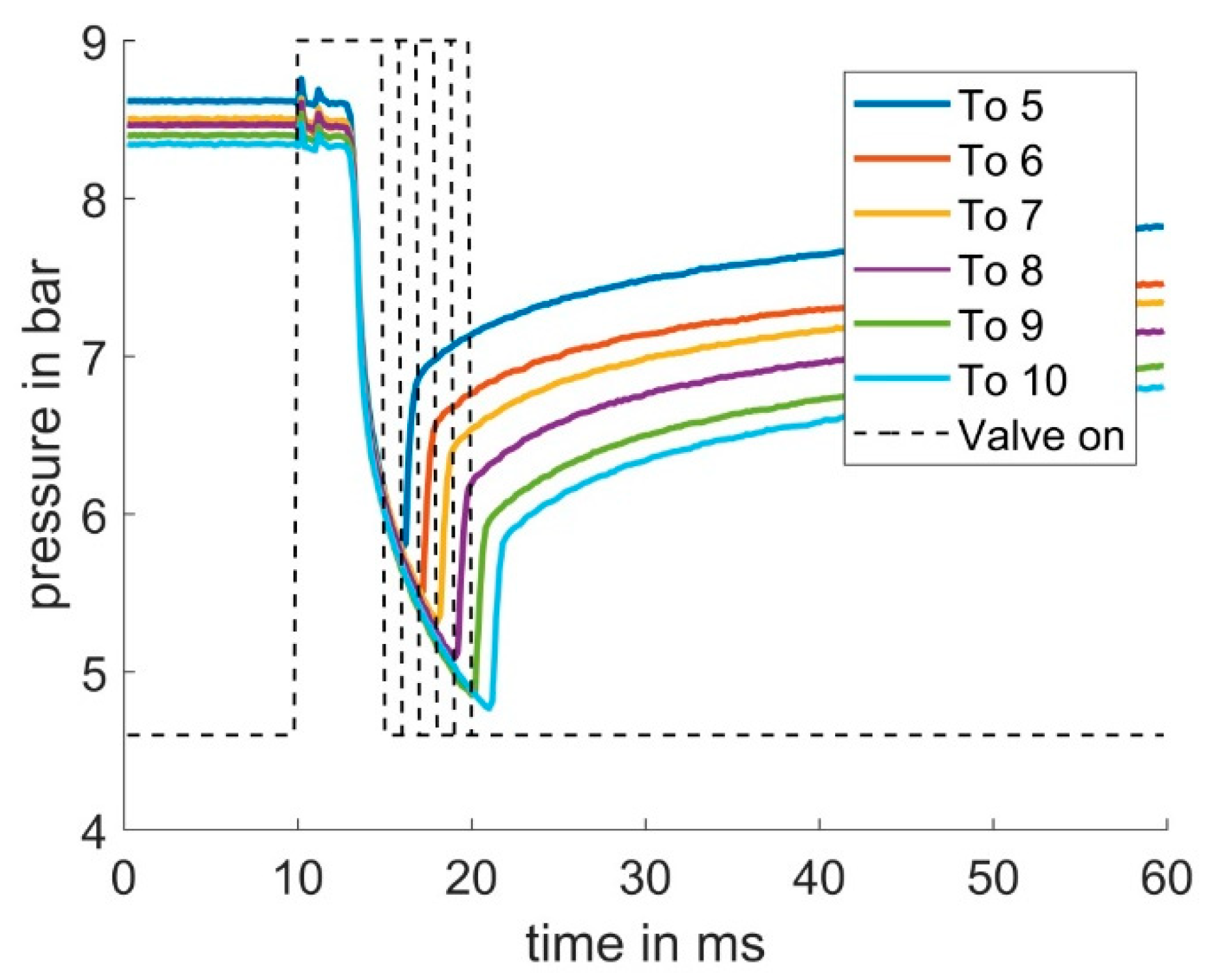
As shown in Figure 3, the grease pressure curve shows a delay of approximately 3 ms after the valve receives its “open” signal. This delay is due to the mechanical upward movement of the pin required to open the valve outlet. When the valve reaches its fully open position, a rapid pressure drop occurs as the compressed material is expelled. This rapid pressure drop is followed by a slower, time-delayed pressure drop. After receiving the closing signal, the pin experiences an additional mechanical delay of approximately 1 ms before closing. As a result, the pressure continues to fall even after the closing signal has been sent. Once the pin has completely closed the valve’s outlet, there is a rapid pressure rise which then transitions into a slower pressure increase.

2.4. Feature Selection

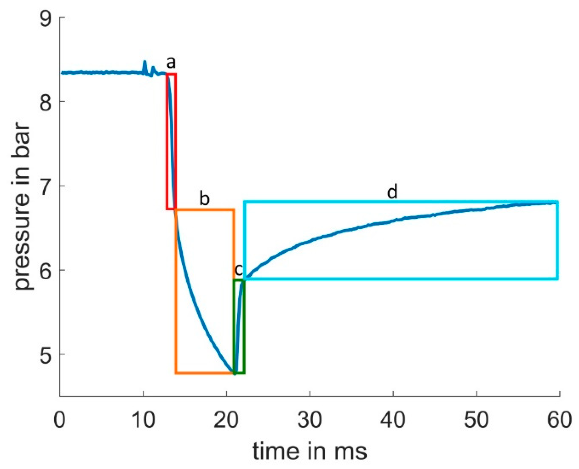
Based on the shape of the pressure curve, nine key features were extracted: the lowest pressure reached, the slope of the fast pressure drop, the approximated T1 time constant for the slow pressure slope, the slope of the fast pressure inclination, and finally the approximated T1 time constant for the slow pressure regeneration phase. The selected areas are shown in Figure 4. The pressure curve was used to extract 16 features in total. These areas of interest correspond to the locations a, b, c, and d from Figure 4. If the feature was during the “on” time of the pulsing valve (when the valve was opened and ejected grease) the name of the feature includes “On”, which corresponds to all features extracted from areas a and b of Figure 4. Features extracted during the “off” time of the valve (when the valve is closed, no grease is ejected, and pressure builds up) include “Off” in their name. Features that are extracted during the phase of rapid decline and increase in pressure (Figure 4a,c) include “K” in their name. Features that are extracted during the slow decline or increase phase (Figure 4b,c) include “T1” in their name. This understanding is mandatory to understand the origin of the features in Table 1.
Based on these areas of interest, three types of feature categories exist. Firstly, constants such as the aforementioned slopes and time constants; secondly, areas such as the area under the pressure curve shown in Figure 5 and the pressure difference curve; and thirdly, the pressure differences.
The pressure curve and the pressure difference–time area curve allow the extraction of features used for prediction. Table 1 lists all available features from the observation. The features are divided into system input, scale, optical and pressure-curve-based features.
The optical column describes the optical features of the pulsed lubricant application process. This involves shooting a small amount of lubricant onto a specimen and then taking a picture of it. The lubricant sticks to the specimen and a camera image is taken to analyze the shape (width and length).
The column scale describes the mass of the feature. The mass of lubricant ejected is measured using a precision scale. Typically, 15 points of lubricant are ejected and then the average mass is calculated.
The column pressure curve is divided into three sub-columns. Pressure difference describes the pressure difference of certain parts of the curve (see Figure 4). Pressure area describes the area under certain points of the curve (see Figure 5) and constants describe the time constants and gains of a hypothetical PT1 element that roughly approximates the curve. A more detailed description of each characteristic can be found in Abbreviations.
Even though all parameters are measured for the analysis of the pressure curve only the columns system input and pressure curve are relevant and therefore used in this paper.

2.5. Predictive Neural Networks and Probability

A specific set of neural networks was created for each predicted feature. As all the networks follow the same architecture, this section describes the general architecture and delves into the details of training one feature as a representation for all the others.
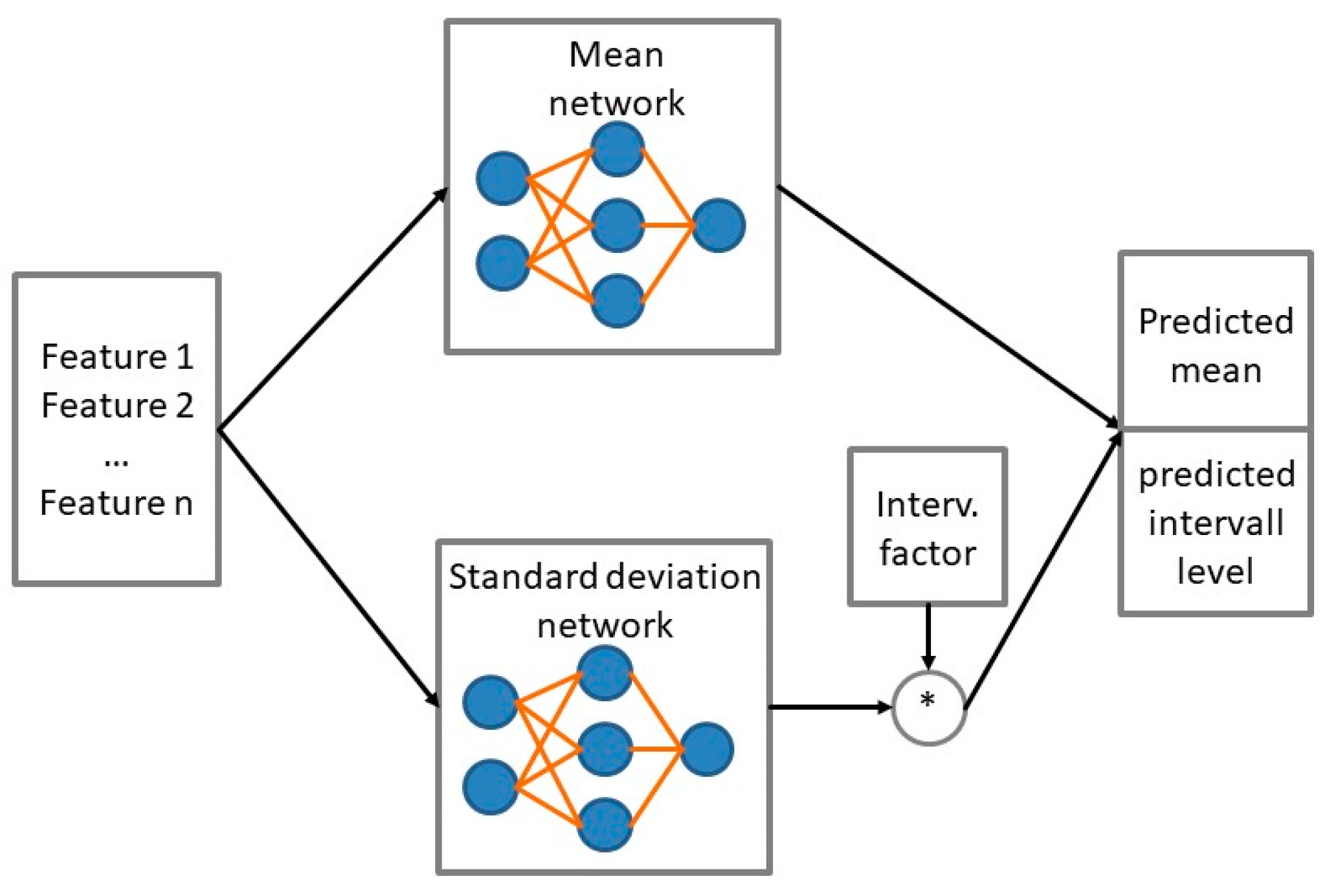
Classical feed-forward neural networks are good at fitting both smooth and noisy data. Ref. [10] shows and analyses the inherent noise tolerance of feed-forward networks. In our case no additional noise reduction methods were used. Typically, the hyper-parameters of the neural network are set to fit the noisy data with the least amount of approximation error. However, a problem arises when the noise is also to be learned. In this case, increasing the number of neurons or layers would cause the network to overfit and produce less generalized solutions. This problem is often referred to as the bias variance dilemma and is discussed in more detail in [11]. In order to learn the bias of the parameter and still be able to predict the standard deviation of the measured features, two neural networks were created. Figure 6 shows the system architecture of the neural network. In our case we decided to use a multilayer feed-forward perceptron network with one hidden layer. Ref. [12] gives a introduction to multilayer feed forward networks and their limitations. Since we predict only parameters and have no need to memorize the timely order of inputs a recurrent network was not necessary.
One neural network is trained with the mean of the measured feature as the target. The second neural network will be trained with the standard deviation of the feature. Therefore, the architecture of both neural networks will be rather lean.
The mean network output is used to track the general trend of the feature, and the standard deviation network output can be used to predict the upper and lower limits of the feature. If a specific interval for the feature is desired, the output of the network can simply be multiplied by a. The result of this architecture will be both the predicted mean and the predicted standard deviation. As input to the neural networks, the valve process parameters already described in Section 2.2, including the pressure curve, are used.

2.6. Training Process

The training data first went through a two-stage standardization and normalization process. Ref. [13] describes and compares both methods for feed-forward network architectures. The test bench is used to generate raw features. These features are then pre-processed in a two-step process. First, the raw data are standardized with a mean of 0 and a standard deviation of 1. The pre-processed data are divided into 70% training, 15% test and 15% validation data. Levenberg–Marquardt backpropagation (see [14] for a deeper explanation) was chosen as the training algorithm since it is a typical training algorithm for neural networks and similar estimation problems (for example [15]). These data will then be used in the training process of the neural networks. Finally, the result will be evaluated and, if necessary, the architecture of the network will be updated by adding or removing neurons or layers.
Experiments have shown that for most features in the mean network, three to ten hidden neurons produce a satisfactory result. If the number of neurons is below two, the network was not able to generalize the feature values accurately enough. The standard deviation network was defined with ten neurons and one hidden layer.
For the mean network, there are two ways of using data to train it. The first possibility is to calculate the average values of all corresponding measurements and then use the average values to train the network. To do this, the average of all measurements with the same system input parameters was calculated, which helped to reduce the amount of data from 8670 to 196 measurements. This reduction speeds up the training process. As the network is only trained with the average values, the entire measured dataset can be used as a test set. This network will be referred to as a “mean network”. A disadvantage of this method is that the use of mean values averages out certain physical effects. Using only the mean values for training results in a smoothing of the pressure values. This can be a disadvantage as peaks and valleys can be averaged out.
To be able to learn these types of effects, it is also possible to train the neural network directly on the measured data. This network will be referred to as a “full network”. The advantage of this method is a higher accuracy in the learned data, since peaks and valleys in the curves are not smoothed. The disadvantage is a longer training time and a smaller test set compared to the first method. Thus, the first method can be seen as more stable in a steady-state calculation. It calculates the average feature that results when multiple grease shots are made. The second method can be seen as a more dynamic solution when each shot needs to be analyzed. Depending on the requirements, a combination of both methods can be used.
The standard deviation network was trained using the calculated standard deviations based on the measurements. Measurements with the same input parameters such as pressure setpoint, temperature setpoint, valve opening time, and valve pin tension were grouped and used to calculate the deviation.

3. Results

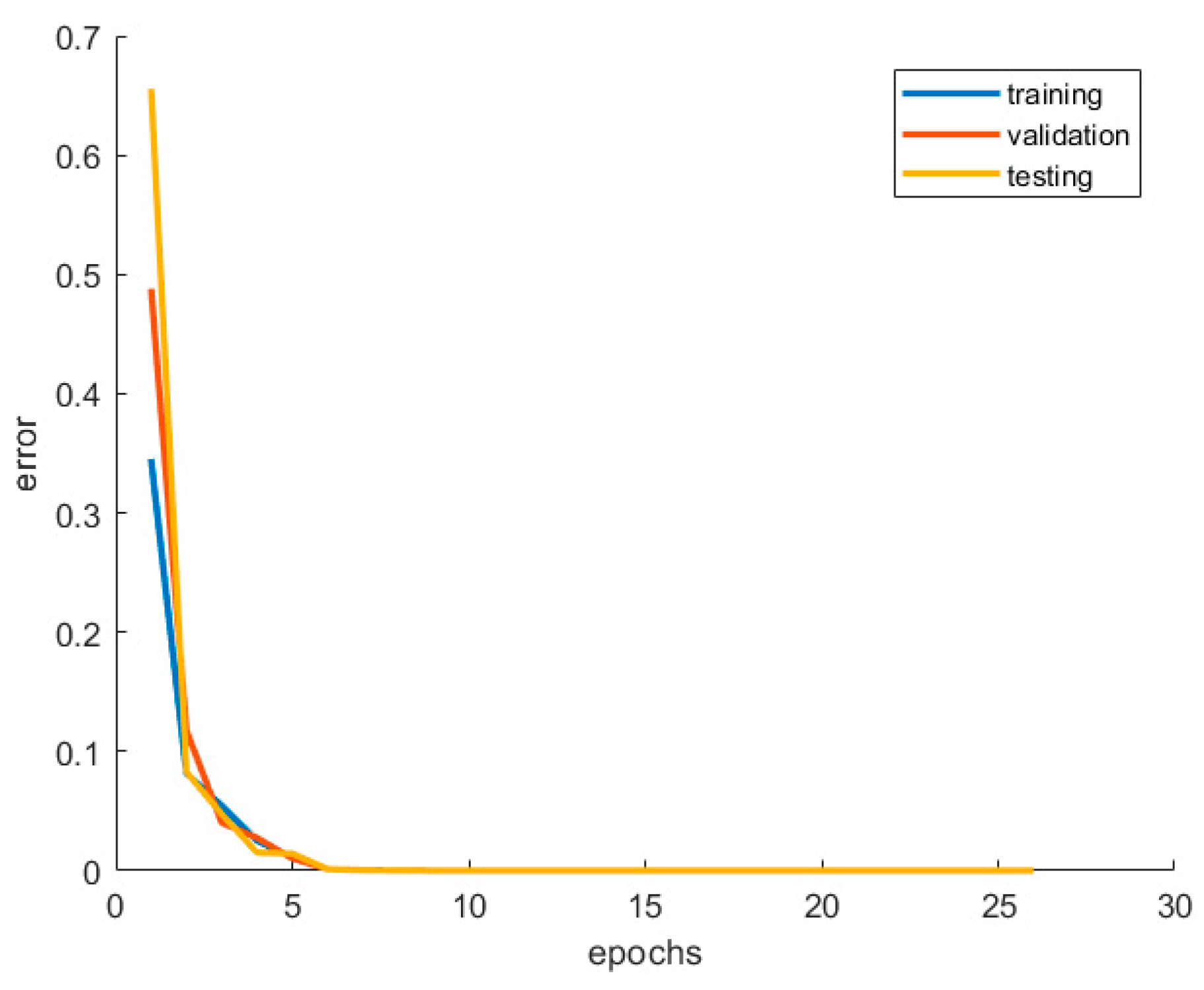
Finding the right number of neurons for the neural network training process was achieved by testing different network configurations. Figure 7 shows an example of the training progress for an exemplary feature called “areaT1OffFull”. The training finishes after 26 epochs without any increase in the error of the test set. Therefore, it can be concluded that the network has managed to generalize the dataset in a satisfactory way.
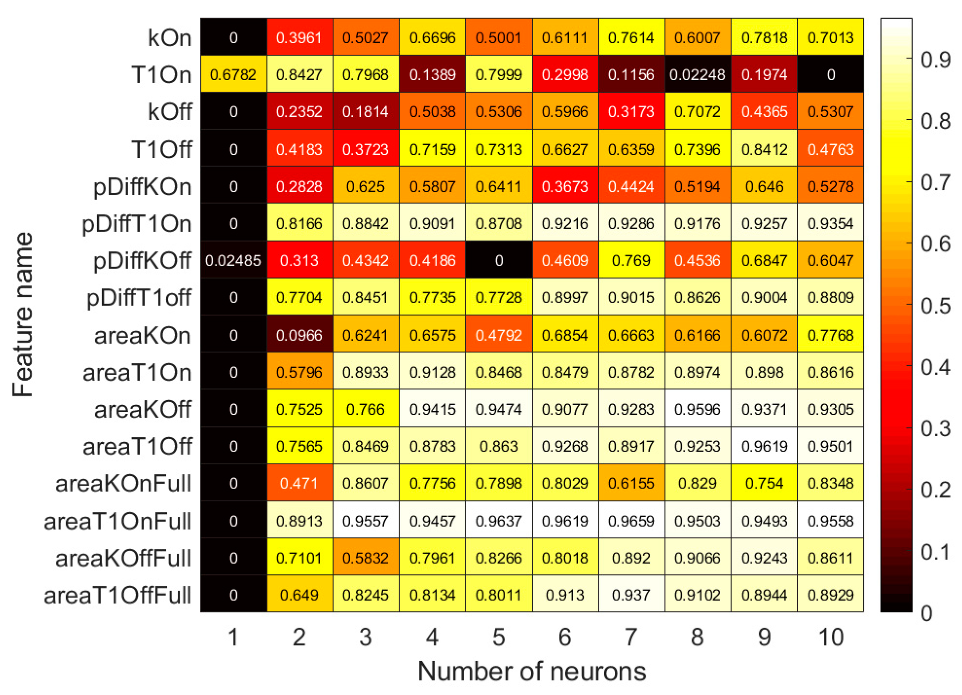
Figure 8 shows the results of the training process for each feature used by the mean network. Each column shows the best network out of 100 trained networks per feature. The features were evaluated with 1 to 10 neurons. In total, 16,000 networks were trained and compared. The result of the test set was normalized between 0 and 1, where 0 means high error and 1 means low error. Smooth features, such as most area features, usually show a rapid increase in performance as the number of neurons increases. Noisy features, such as pressure curve time constants and slopes, have a noisier performance as the number of neurons trained increases. For all features, a single neuron could not approximate the data accurately enough. Feature T1On was the only one that had the best approximation with only two neurons.
Figure 9 displays the training process result of the full network. Because the network was trained with a greater dataset (8670 data points) and without any averaging to smoothen the noise, up to 20 neurons were compared. The general outcome is similar to the mean network, most of the area features again show a smooth increase in performance. Noisy features such as KOn show a higher fluctuating performance measure. In general, the full network performs better by having more neurons than the mean networks.
Figure 10 shows the comparison of two features, F1 and F10. In both cases it appears that the resulting fit is closer to an average value of the curve. The full network fit of F1 is 6.7% better than the mean networks. In the case of F10, the full network fit is approximately 1.1% better than the mean networks.
After both mean and full networks are trained, they will be combined with the standard deviation network to calculate the upper and lower boundaries of the regression value. Figure 11 shows a 1-sigma interval for F1 for both networks. The result using the full network appears to have a higher variance than the mean network. This can be seen in Figure 11c,d where 1500–1600 samples are shown. The reason for the lower variance of the mean network is the smoothing effect of the mean network, as both networks use the same standard deviation network. The mean absolute error (MAE) also supports this assumption. The mean network has an MAE of 0.0398 for the feature KOn, while the full network has a lower MAE of 0.0381 over all samples.

4. Discussion

Both the mean network and the full network are compared in terms of their performance. To create a valid comparison, 30% of the total dataset was randomly extracted as a new test set. The mean network was trained with its original mean values, the other network was trained with the remaining 70% of the dataset. Both types of networks were trained with their calculated best number of neurons. The coefficient of determination (R2) is used to assess the fit of the networks and to compare them. R2 measures how much of the variance in the dependent variables can be explained by the independent variables. An R2 value close to 1 indicates that the independent variables of the model can explain the variance of the measured values well, while an R2 value close to 0 means the opposite. The closer R2 is to 1, the better the model fits the data. Table 2 shows the training result: the R2 value of each feature and each net is shown. Smooth features like F3, F4, F7, F8, and F10–F16 can be trained very well with both neural networks. The remaining features show both a greater variance in the measured data and a lower R2 value and therefore a poorer fit. The average R2 value over all features of the full network is 0.781 while the mean network’s average R2 value is 0.737.
Finally, the performance of both networks needs to be evaluated. Therefore, for both the mean and the full network, it was calculated how many data points in each feature are within the 1-sigma, 2-sigma, and 3-sigma intervals. The results of this performance evaluation can be seen in Table 3, where features with low noise seem to cover the majority of points inside the boundary even at 1 sigma. Features with higher noise, on the other hand, come closer to the 68% mark. Therefore, it can be concluded that the standard deviation network manages to capture the boundaries of noisy features well. Furthermore, it can be seen that boundaries with the mean network give a lower percentage of included points than the full network. This is understandable as the mean network was trained to approximate the mean, whereas the full network was trained directly on the data.

5. Conclusions

Two pressure curve feature prediction networks have been successfully trained and evaluated on a test set. Both mean and full networks can be used for smooth features. Noisy features can be estimated by adding the standard deviation network to obtain a confidence limit.
One of the limitations of this observation was that temperature was not considered as a control parameter. All measurements were made at room temperature. However, in some production applications heating elements are used to bring the lubricant to specific temperatures and change its viscosity. Another limitation of this work is that the pressure curve is highly dependent on the geometry of the valves and especially the nozzles. The trained networks are therefore only able to predict for the equipment used. However, they can be retrained for other types. Another limitation of this research is the focus on grease as a lubricant. In the current change in mindset and efforts to find more sustainable and less polluting materials for production, the application process of green lubricants such as the PVA/UG composite proposed in [1] should be considered.
The next steps will be to collect more data with different types of valve nozzles and lubricants. A study will be completed to determine if the network architecture is able to learn to identify different types of lubricants and correctly estimate their characteristics. A prediction of the shape and weight of the lubricant will also be concluded. The already trained networks will be used to generate additional training features for regression. In addition, the test stand will be equipped with a valve heating system and a temperature sensor to accurately control and measure the lubricant temperature. This will help to quantify temperature-dependent influences.
This document is the result of the research project “AdaptValve” funded by the German Federal Ministry for Economic Affairs and Climate Action.

Author Contributions

Conceptualization, S.P.; methodology, S.P.; software, S.P.; validation, S.P.; formal analysis, S.P.; investigation, S.P.; resources, S.P.; data curation, S.P.; writing—original draft preparation, S.P.; writing—review and editing, F.F., M.K. and M.H.; visualization, S.P.; supervision, M.K. and M.H.; project administration, S.P. and M.K.; funding acquisition, M.K. All authors have read and agreed to the published version of the manuscript.

Funding

This research was funded by German Federal Ministry for Economic Affairs and Climate Action, Zentrales Innovationsprogramm Mittelstand (ZIM). Open Access Funding by the University of Applied Sciences Technikum Wien.

Institutional Review Board Statement

Not applicable.

Informed Consent Statement

Not applicable.

Data Availability Statement

The original contributions presented in the study are included in the article, further inquiries can be directed to the corresponding author.

Conflicts of Interest

Author Frederic Förster was employed by the Walther Systemtechnik GmbH. The remaining authors declare that the research was conducted in the absence of any commercial or financial relationships that could be construed as a potential conflict of interest.

Abbreviations

Opening timeTo
Temperature set pointTemp
Pressure set pointPreg
Pressure in valveVu
Starting pressuremaxP
Lowest pressure reachedminP
Initial slope during fast pressure dropKOn
Time constant during pressure dropT1On
Initial slope during fast pressure regenerationKOff
Time constant during pressure regenerationT1Off
Pressure–time area during KOnareaKOn
Pressure–time area during T1OnareaT1On
Pressure–time area during KOffareaKOff
Pressure–time area during T1OffareaT1Off
Pressure difference–time area during KOnareaKOnFull
Pressure difference–time area during T1OnareaT1OnFull
Pressure difference–time area during KOffareaKOffFull
Pressure difference–time area during T1OffareaT1OffFull
Pressure difference for KOnpDiffKOn
Pressure difference for T1OnpDiffT1On
Pressure difference for KOffpDiffKOff
Pressure difference for T1OffpDiffT1Off

References

  1. Rahmadiawan, D.; Abral, H.; Shi, S.-C.; Huang, T.-T.; Zainul, R.; Ambiyar, A.; Nurdin, H. Tribological Properties of Polyvinyl Alcohol/Uncaria Gambir Extract Composite as Potential Green Protective Film. Tribol. Ind. 2023, 45, 367–374. [Google Scholar] [CrossRef]
  2. Abral, H.; Ikhsan, M.; Rahmadiawan, D.; Handayani, D.; Sandrawati, N.; Sugiarti, E.; Muslimin, A.N. Anti-UV, antibacterial, strong, and high thermal resistant polyvinyl alcohol/Uncaria gambir extract biocomposite film. J. Mater. Res. Technol. 2022, 17, 2193–2202. [Google Scholar] [CrossRef]
  3. Rudnick, L.R. Synthetics, Mineral Oils, and Bio-Based Lubricants: Chemistry and Technology (Chemical Industries); CRC Press: Boca Raton, FL, USA, 2005. [Google Scholar]
  4. Specht, D.F. Probabilistic Neural Networks for Classification, mapping, or associative memory. In Proceedings of the IEEE International Conference on Neural Networks, San Diego, CA, USA, 24–27 July 1988; IEEE Press: New York, NY, USA, 1988; Volume 1, pp. 525–532. [Google Scholar]
  5. Malone, C.; Fennell, L.; Folliard, T.; Kelly, C. Using a neural network to predict deviations in mean heart dose during the treatment of left-sided deep inspiration breath hold patients. Phys. Med. 2019, 65, 137–142. [Google Scholar] [CrossRef]
  6. Specht, D.F. Probabilistic Neural Networks. Neural Netw. 1990, 3, 109–118. [Google Scholar] [CrossRef]
  7. Othman, M.F.; Basri, M.A.M. Probabilistic Neural Network for Brain Tumor Classification. In Proceedings of the 2011 Second International Conference on Intelligent Systems, Modelling and Simulation, Kuala Lumpur, Malaysia, 25–27 January 2011; pp. 136–138. [Google Scholar]
  8. Camousseigt, L.; Galfré, A.; Couenne, F.; Oumahi, C.; Muller, S.; Tayakout-Fayolle, M. Oil-bleeding dynamic model to predict permeability characteristics of lubricating grease. Tribol. Int. 2023, 183, 108418. [Google Scholar] [CrossRef]
  9. Akchurin, A.; Van den Ende, D.; Lugt, P.M. Modeling impact of grease mechanical ageing on bleed and permeability in rolling bearings. Tribol. Int. 2022, 170, 107507. [Google Scholar] [CrossRef]
  10. Lu, W.; Zhang, Z.; Qin, F.; Zhang, W.; Lu, Y.; Liu, Y.; Zheng, Y. Analysis on the inherent noise tolerance of feedforward network and one noise-resilient structure. Neural Netw. 2023, 165, 786–798. [Google Scholar] [CrossRef] [PubMed]
  11. Geman, S.; Bienenstock, E.; Doursat, R. Neural networks and the bias/variance dilemma. Neural Comput. 1992, 4, 1–58. [Google Scholar] [CrossRef]
  12. Popescu, M.C.; Balas, V.E.; Perescu-Popescu, L.; Mastorakis, N. Multilayer perceptron and neural networks. WSEAS Trans. Circuits Syst. 2009, 8, 579–588. [Google Scholar]
  13. Shanker, M.; Hu, M.Y.; Hung, M.S. Effect of data standardization on neural network training. Omega 1996, 24, 385–397. [Google Scholar] [CrossRef]
  14. Hagan, M.T.; Menhaj, M.B. Training Feedforward Networks with the Marquardt Algorithm. IEEE Trans. Neural Netw. 1994, 5, 989–993. [Google Scholar] [CrossRef] [PubMed]
  15. Lv, C.; Xing, Y. Levenberg-Marquardt Backpropagation Training of Multilayer Neural Networks for State Estimation of A Safety Critical Cyber-Physical System. IEEE Trans. Ind. Inform. 2018, 14, 3436–3446. [Google Scholar] [CrossRef]
Figure 1. Schematic setup of automated test stand.
Eng 05 00127 g001
Figure 2. Grease application process sample in pulsing mode, 15 grease test points where taken, grease type Berulub Fr16, grease pressure controller 20 Bar setting, 7 ms opening time of valve, 30 clicks on pin tension setting.
Eng 05 00127 g002
Figure 3. Average pressure curves with varying valve opening time To. Every curve was averaged by 15 curves which were produced during the application process. The general curve’s shape tends to stay constant, the varying starting pressure results from the grease’s time-dependent system behavior.
Eng 05 00127 g003
Figure 4. Pressure curve areas of interest for feature selection. (a) Rapid decline of pressure after valve is opened. (b) Slowing decline of pressure after valve is opened. If the valve continues to be open then a steady state pressure would be reached. (c) Rapid increase in pressure after valve is closed. (d) Slower increase in pressure after valve is closed. A steady state is reached if the valve continues to be closed.
Eng 05 00127 g004
Figure 5. Pressure curve area features extracted according the defined areas of interest. The picture above shows the pressure–time area, while the picture below shows the pressure difference–time curve. Both cases are shown for a pulsing and regeneration process.
Eng 05 00127 g005
Figure 6. Neural network system architecture.
Eng 05 00127 g006
Figure 7. Error of training, validation, and test sets for feature areaT1OffFull using 6 neurons.
Eng 05 00127 g007
Figure 8. Comparison of training result depending on number of neurons for all features of the mean network. Light-colored values indicate a good score, dark-colored features indicate a worse score.
Eng 05 00127 g008
Figure 9. Comparison of training result depending on number of neurons for all features of the full network. Light-colored values indicate a good score, dark-colored features indicate a worse score.
Eng 05 00127 g009
Figure 10. Comparison of feature KOn (F1) and areaT1On (F10) fit.
Eng 05 00127 g010
Figure 11. Calculated network regression with added boundary from the standard deviation network for the same feature KOn. (a) Full network over all samples. (b) Mean network over all samples. (c) Full network zoomed in. (d) Mean network zoomed in.
Eng 05 00127 g011
Table 1. Table of all features.
Feature Table
OpticalScaleSystem InputPressure Curve
Pressure DifferenceAreasConstants
widthmassTopDiffKOnareaKOnkOn
height TemppDiffKOffareaT1OnkOff
VuPDiffT1OnareakOffT1On
PregPDiffT1OffareaT1OffT1Off
maxP Area-KOnFull
minPArea-KT1OnFull
Area-KOffFull
Area-KOnFull
Table 2. Coefficient of determination for all features.
Coefficient of Determination
FeatureF1F2F3F4F5F6F7F8
Full net0.4020.1310.8950.7600.4810.6430.8880.983
Mean net0.3350.1790.8830.7160.4200.6310.8730.918
FeatureF9F10F11F12F13F14F15F16
Full net0.3710.9980.9600.9860.9951.0000.9961.000
Mean net0.3050.9870.9190.6340.9950.9970.9940.998
Table 3. Percentage of test points in boundary.
Percentage of Test Points in Boundary
Feature F1 F2 F3 F4 F5 F6 F7 F8
Full Isig 72% 51% 76% 76% 69% 74% 75% 68%
Full 2sig 96% 74% 94% 94% 96% 96% 93% 93%
Full 3sig 98% 85% 96% 97% 99% 98% 96% 98%
Mean lsig 70% 44% 75% 71% 68% 72% 74% 51%
Mean 2sig 95% 64% 93% 92% 95% 95% 93% 79%
Mean 3sig 98% 77% 97% 96% 98% 99% 96% 91%
Feature F9 F10 F11 F12 F13 F14 F15 F16
Full Isig 74% 84% 72% 87% 90% 89% 86% 92%
Full 2sig 96% 97% 97% 97% 98% 97% 97% 98%
Full 3sig 99% 99% 99% 98% 99% 99% 98% 98%
Mean Isig 73% 62% 62% 75% 88% 73% 81% 81%
Mean 2sig 95% 84% 90% 91% 98% 92% 96% 93%
Mean 3sig 98% 92% 95% 94% 99% 95% 97% 96%
Disclaimer/Publisher’s Note: The statements, opinions and data contained in all publications are solely those of the individual author(s) and contributor(s) and not of MDPI and/or the editor(s). MDPI and/or the editor(s) disclaim responsibility for any injury to people or property resulting from any ideas, methods, instructions or products referred to in the content.