Abstract
Navigation poses a significant challenge for autonomous vehicles, prompting the exploration of various bio-inspired artificial intelligence techniques to address issues related to path generation, obstacle avoidance, and optimal path planning. Numerous studies have delved into bio-inspired approaches to navigate and overcome obstacles. In this paper, we introduce the dragonfly algorithm (DA), a novel bio-inspired meta-heuristic optimization technique to autonomously set goals, detect obstacles, and minimize human intervention. To enhance efficacy in unstructured environments, we propose and analyze the dragonfly–fuzzy hybrid algorithm, leveraging the strengths of both approaches. This hybrid controller amalgamates diverse features from different methods into a unified framework, offering a multifaceted solution. Through a comparative analysis of simulation and experimental results under varied environmental conditions, the hybrid dragonfly–fuzzy controller demonstrates superior performance in terms of time and path optimization compared to individual algorithms and traditional controllers. This research aims to contribute to the advancement of autonomous vehicle navigation through the innovative integration of bio-inspired meta-heuristic optimization techniques.
1. Introduction
The rapid evolution of the logistics industry has spurred the demand for intelligent autonomous vehicles to enhance efficiency and streamline processes [1]. The substitution of human labor in labor-intensive, repetitive, and hazardous tasks with autonomous vehicles has garnered significant attention and proven vital for optimizing operational efficiency and resource utilization in modern factories and warehouses [2]. An autonomous vehicle is characterized as an intelligent entity capable of perceiving its surroundings, collecting and analyzing pertinent information from sensors, and determining its current position. Additionally, such a vehicle can generate a viable path from its initial location to the target destination by employing decision control mechanisms to navigate along a planned trajectory [3]. Path-planning methods play a pivotal role in realizing the intelligence of autonomous vehicles and entail the determination of an optimal path from the starting point to the destination in intricate spatial environments. This involves considering the initial and target positions provided during vehicle operation [4]. Path-planning problems are categorized into static and dynamic environments and address challenges related to both static and dynamic obstacle avoidance [5,6].
Path-planning algorithms play a prevalent role in both outdoor and indoor navigation scenarios. Various navigation and motion-planning techniques, including classical approaches, heuristic methods, and bioinspired algorithms, have been employed in the realm of autonomous vehicle technologies, specifically within the context of pathfinding algorithms. Classical path-planning methods such as A*, RRT, and PRM, characterized as traditional approaches, have been extensively utilized and studied to address path-planning challenges across diverse domains. These methods have demonstrated their efficacy in discovering viable paths within known environments and established themselves as foundational elements in the field of path-planning research over an extended period. A* [7] is a popular heuristic search algorithm that guarantees an optimal path in a discretized state space, making it efficient for small and structured environments. RRT [8,9] (rapidly-exploring random trees) is a sampling-based algorithm that efficiently explores high-dimensional spaces and has shown promise in handling complex and dynamic environments. PRM (probabilistic roadmap) [10] is another sampling-based technique that constructs a roadmap of the configuration space and enables quick path-planning by connecting waypoints. Although traditional methods have their merits, bioinspired algorithms offer distinct advantages that make them superior for certain path-planning scenarios. Bioinspired algorithms, inspired by natural systems, emulate collective behaviors to solve optimization problems. These algorithms possess several strengths that set them apart from traditional methods: robustness in complex environments, a balance of exploration–exploitation, handling of dynamic environments, scalability, and flexibility in parameter tuning. In dynamic environments where obstacles or target locations change over time, bioinspired algorithms can dynamically adapt their search strategies, making them more suitable for real-time applications. Additionally, their stochastic nature enables a good balance between exploration and exploitation, which allows them to escape local optima and find better global solutions in uncertain environments.
Bio-inspired algorithms, or biologically inspired algorithms, constitute a specialized category of stochastic and metaheuristic search algorithms within the realm of computational sciences. Recognized for their effectiveness in addressing distributed and multimodal optimization problems [11], these algorithms employ robust search procedures that facilitate diversity maintenance, steering clear of local optimal convergence and increasing the likelihood of achieving globally optimal solutions [12,13]. The concern over the lack of control in exploration noises is inherent in bio-inspired methods, which prompts strategies to incorporate exploratory behavior through noise injection into the action space or agent parameters and fosters more reliable exploration and a wider range of behaviors. Bio-inspired algorithms, which foster agent interactions and leverage feedback mechanisms for cooperative dynamics, find applications in various scientific and engineering domains such as data mining and neural networks. Specifically applied to path optimization for autonomous vehicles, a range of swarm intelligence algorithms, including ant colony optimization (ACO) [14], particle swarm optimization (PSO) [15], the firefly algorithm (FA) [16], the fruit fly algorithm (FFA) [17], the bat algorithm [18], grey wolf optimization [19], and the grasshopper optimization algorithm (GOA) [20], contribute collectively to addressing diverse navigational challenges encountered by autonomous vehicles.
However, the existing path-planning algorithms have certain limitations, especially when dealing with multi-objective optimization and navigating in unstructured environments. In real-world scenarios, it is essential to consider multiple elements simultaneously, such as travel distance, collision safety, and path flexibility, rather than focusing on just one component. Hybrid approaches that combine bioinspired algorithms with heuristic techniques, such as A* [21] and fuzzy logic [22], have shown promise in improving the efficiency of autonomous vehicles. For instance, the A*–fuzzy hybrid approach optimizes the shortest path while avoiding obstacles [23], and quarter orbits particle swarm optimization (QOPSO) ensures an optimal path free of collisions [24]. However, these hybrid approaches still face challenges, such as high power consumption and unsmooth paths, when considered independently.
Fuzzy logic control and inferencing systems have been applied in various path-planning methods, as demonstrated in prior research [25]. This soft-computing approach allows for the utilization of knowledge represented in linguistic rules [26], which enables the incorporation of expert human knowledge and experience, particularly in obstacle avoidance scenarios [27]. Fuzzy logic is well suited for handling imprecise variables and uncertainties, making it capable of addressing unknown conditions and dynamically reacting to changing environments [28]. As a result, it serves as an ideal tool to tackle obstacle avoidance problems effectively. The dragonfly algorithm (DA) [29] has been extended to and applied in various optimization tasks. A binary version of the algorithm (BDA) was proposed for solving the 0–1 knapsack problem [30] and showcased strong convergence and stability. In the context of feature selection, modified versions of BDA were introduced that incorporated penalty functions [31] and other methods to enhance performance. The integration of time-varying transfer functions into BDA demonstrated its effectiveness in feature selection tasks, outperforming other algorithms on benchmark datasets [32]. Additionally, DA has been utilized for swarm mobile robots with obstacle avoidance and showed efficiency in rescue scenarios [33]. Chaotic dragonfly algorithm (CDA) variations incorporated chaos to accelerate convergence in feature selection tasks [34], and the adaptive dragonfly [35] algorithm (ADF) was presented as a self-adaptive approach for multilevel segmentation by achieving superior solutions compared to standard DA and other optimization techniques. These diverse variants and applications highlight the versatility and performance of DA in solving different optimization challenges.
The task of autonomous vehicle path planning holds significant importance, as it aims to determine the optimal trajectory under diverse circumstances. This involves generating real-time high-quality paths while considering factors such as path quality, efficiency, and computational resource consumption. Ji et al. [36] introduced an innovative method employing a 3-D virtual dangerous potential field to navigate potential collisions, relying on complex calculations of collision-free trajectories. Simultaneously, obstacle avoidance, which is crucial for vehicle safety, requires careful consideration of dynamic and static obstacles, vehicle-maneuvering capabilities, comfort, and handling stability. To address conflicts arising from various objectives, inventive control structures such as Fernando et al.’s MIMO method for autonomous vehicle path tracking address network-induced delays and incorporate roll dynamics to enhance safety and passenger comfort [37]. Path-tracking control is essential for guiding actuators along the planned route by utilizing various algorithms such as PID-based, feedforward and feedback, model predictive control (MPC), robust control, and optimal preview methods for automated ground vehicles [38]. The interaction between path-tracking control and vehicle dynamics control presents a central challenge. Hu et al. [39] and Chen et al. [40] introduced output constraint controllers and simultaneous path-following and lateral stability control methods, respectively. However, there remains a need for real-time simulation evaluations and practical experimentation to validate the efficacy of these approaches.
To address the challenges and improve path-planning efficiency for autonomous vehicles operating in static and dynamic environments, this study introduces a novel strategy termed the dragonfly–fuzzy hybrid approach. This method harnesses the collective intelligence of the dragonfly algorithm and the adaptability of fuzzy logic to identify the most direct collision-free path. The proposed dragonfly–fuzzy algorithm provides an innovative solution that takes into account both obstacle avoidance and the optimization of path length. Through the integration of bioinspired, traditional, and hybrid techniques, our approach aims to deliver a path-planning solution that is both efficient and effective. Comparative analysis against standalone algorithms illustrates the superior performance of the dragonfly–fuzzy hybrid strategy in terms of optimizing path length and computational time. This research represents a promising advancement in autonomous vehicle path planning, particularly in unstructured environments, contributing to ongoing efforts to enhance navigation and motion planning in the field of autonomous vehicles.
2. Path-Planning Algorithms
The key issue with moving an autonomous vehicle from one position to another is identifying the best or close to the best desired path by avoiding obstacles in order to reach the target with desirable accuracy. Hence, the most crucial function of any navigational technique is safe path planning along with obstacle avoidance from the initial place to the target position. As a result, when working in a simple or complex environment, the proper selection of the navigational strategy is the most critical phase in the planning of an autonomous vehicle’s course. This study used fuzzy logic and the dragonfly algorithm for path planning and autonomous mobile robot obstacle detection.
2.1. Dragonfly Algorithm
In 2015, Seyedali Mirjalili introduced the dragonfly algorithm [29] as a solution to address multi-objective optimization challenges. The inspiration for the dragonfly algorithm (DA) was drawn from swarming behaviors related to static and dynamic scenarios, mirroring the exploration and exploitation phases inherent in metaheuristic optimization. Static swarming behavior, referred to as hunting, involves a small group of dragonflies swiftly adjusting their movements in search of food. On the other hand, dynamic swarming, known as migratory swarming, involves a large group of dragonflies covering extensive distances for migration. These swarming behaviors, in line with Reynolds’ concepts from 1987, encompass separation, alignment, cohesion, attraction to food, and distraction from opponents. The dragonfly algorithm is designed to emulate these social interactions, incorporating two primary optimization phases: exploration and exploitation. Various versions of the algorithm, such as the binary dragonfly algorithm (BDA), multi-objective dragonfly algorithm (MODA), and single-objective dragonfly algorithm (SODA), cater to dynamic navigation, food hunting, and engaging enemies in a compiled manner.
The fundamental principles governing the dragonfly algorithm encompass five core rules: separation, alignment, cohesion, attraction, and distraction. The population size, denoted as M, serves as an indicator of the total number of individual dragonflies. The position of the dragonfly is defined as
In the given context of , denotes the dragonfly’s position within the dimension of the search space, and M corresponds to the total number of search agents. The symbol signifies the position of the current individual fly.
- The dragonfly algorithm’s segregation principle pertains to the internal avoidance of collisions with other individuals within the algorithm’s proximity. This concept is expressed mathematically in Equation (2).
- 2.
- The concept of alignment () in the given context signifies the synchronization of velocities among neighboring individuals within the same group. This mathematical representation is given in Equation (3).
In this context, as the term “alignment motion” denotes the motion of the current individual “i” at the iteration. Similarly, is the velocity of the neighboring individual “j” at the iteration.
- 3.
- Cohesion in this context signifies the inclination of individuals to move towards the center of the mass within their neighborhood. This tendency is expressed mathematically, as illustrated in Equation (4).
In this scenario, is the term “cohesion motion”, referring to the movement of the present individual “i” during the iteration.
- 4.
- Attraction in this context signifies the food source, which is mathematically represented in Equation (5).
In the above scenario, the term represents the food source at the iteration and represents the food attraction motion of the current individual “i”.
- 5.
- Distraction represents the distraction from the enemy as shown in the Equation (6).
In this context, represents the enemy position at iteration. The distraction of the enemy is represented by for the current individual “i” at the iteration.
Regarding the dragonfly’s position, its entities share similarities with the step vector update characteristic observed in the particle swarm optimization method [41]. In this context, the step vector () and the position vector () assume crucial roles in adapting the dragonflies’ positions within the exploration domain, effectively directing their movements. The step vector delineates the direction of the dragonflies’ motion, whereas the position vector defines the specific locations of individual dragonflies in the exploration space. The computation of the step vector follows the subsequent formula.
In this context, the symbol represents the current step vectors denoting separation, indicates alignment, represents cohesion, signifies the influence of the food source, and represents a distraction. Additionally, is the inertia weight. Initially, each operator is assigned initial weights through a random process, and subsequently, these weights are dynamically adjusted to facilitate the convergence of dragonflies towards an optimal solution. Following the computation of the step vector, the position vector can be determined using the following procedure.
In the above equation, represents the current iteration, the next position is represented by , and represents the current position.
As the optimization process advances, the dragonfly’s neighborhood radius undergoes expansion. When the dragonfly has at least one neighboring entity, the procedures involving () and () come into play to update its velocity and position. Nevertheless, in instances where the dragonfly algorithm encounters situations without any neighbors, it resorts to a random movement strategy. During such occurrences, the Levy flight technique is applied to adjust both the position and the velocity of the dragonflies. The incorporation of the Levy flight technique introduces heightened levels of randomness and chaotic behavior, thereby augmenting the algorithm’s global search capabilities. In this particular circumstance, the position undergoes an update using Levy flight, as outlined in Equation (9).
In the above context, the number of decision variables is represented by “d”, whereas the Levy flight function is denoted by “Levy(d).”
The main objective of using the dragonfly algorithm (DA) is to navigate an autonomous vehicle in an unstructured environment consisting of different obstacles. This objective is transformed into a minimization problem with two functions. The first is to avoid obstacles, and the second is to find the shortest possible path. Figure 1 depicts the environment of the autonomous vehicle’s target and goal positions.
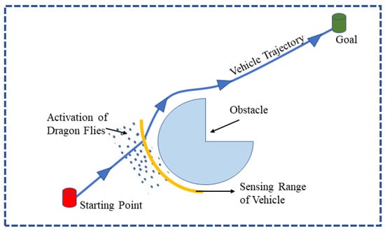
Figure 1.
Autonomous vehicle positioning in the presence of an obstacle.
Figure 2 depicts the architecture of the proposed DA controller, and Algorithm 1 illustrates the pseudo-code for the DA to describe its execution.
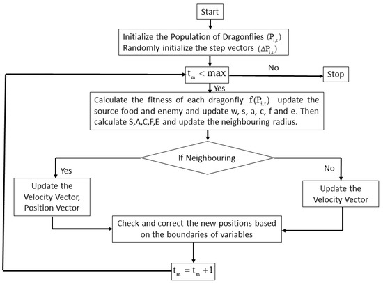
Figure 2.
Dragonfly algorithm architecture.
The dragonfly algorithm is a metaheuristic approach that stands as an optimization technique inspired by the collective behavior of dragonflies. Its initiation involves the setup of a dragonfly population along with their corresponding step vectors. The algorithm iteratively computes the objective values of dragonflies while dynamically adjusting parameters such as food source, enemy, separation, alignment, cohesion, attraction, and distraction. Adjustments to the neighborhood radius are applied, and if a dragonfly has at least one neighboring counterpart, updates are made to both the velocity vector and the position vector. To enhance adaptability, the algorithm integrates Levy flight for position adjustments and conducts boundary checks for corrections. Exhibiting efficiency and scalability, the dragonfly algorithm boasts a time complexity of O(N), where N denotes the number of iterations. The standard algorithm steps are outlined as follows.
| Algorithm 1 Dragonfly Algorithm |
| # Dragonfly algorithm # Complexity analysis: O(N), where N is the number of iterations def dragonfly_algorithm(): # Initialization population = initialize_population() step_vectors = initialize_step_vectors() # Iterative optimization loop while not end_condition_satisfied(): # Objective value calculation calculate_objective_values(population) # Update food source and enemy update_food_source_and_enemy() # Update factors: separation, alignment, cohesion, food, and enemy update_factors() # Calculate and update vectors using equations calculate_and_update_vectors() # Update neighboring radius update_neighboring_radius() # Update position and velocity vectors based on neighbors for dragonfly in population: if dragonfly_has_neighboring_dragonflies(dragonfly): update_velocity_and_position(dragonfly) else: update_position_levy_flight(dragonfly) # Check and correct new positions based on variable boundaries check_and_correct_positions(dragonfly) # End of the algorithm # Time complexity: O(N), where N is the number of iterations |
2.2. Fuzzy Logic Concept
The inception of fuzzy logic methodologies was introduced by Lotfi Zadeh in 1965 [42]. This approach draws inspiration from human decision-making, encompassing nuanced responses beyond binary choices like yes or no. Fuzzy logic addresses multifaceted scenarios by employing if–else rules, which capture the essence of complex decision processes. It operates by processing imperfect and non-uniform data across various concerns. Unlike conventional linear logic, fuzzy logic adeptly handles intricate data challenges characterized by substantial uncertainty. The fundamental framework of fuzzy logic is depicted in Figure 3.
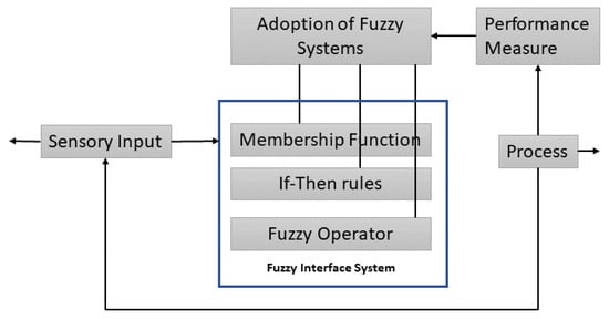
Figure 3.
Schematic diagram of fuzzy logic.
The fundamental elements of fuzzy logic encompass several crucial facets:
- •
- Fuzzification: This involves employing membership functions to delineate input variables.
- •
- Inference and aggregation: This factor determines the final output resulting from fuzzy rules, accomplished through a process of inference and aggregation.
- •
- Defuzzification: The transformation of fuzzy-based output into a precise value is achieved through the process of defuzzification.
The core principle of fuzzy inference revolves around elementary mapping strategies that use input data to produce output variables. Within fuzzy inference, the crucial utilization of if–then rules plays a central role and forms the basis for the decision-making process. Let the various objects denoted by “x” be represented by and “x”, forming a known pair for the fuzzy set “A”.
As depicted in Equation (10), the fuzzy membership function is defined by for set A. The membership function maps for membership space M, i.e., .
In the interval [0, 1] lies the membership values, which indicate the range of the membership function with a subset of non-negative real numbers. The fundamental problem in fuzzy logic is addressed through two types of functions, namely, trapezoidal and triangular. Equation (11) delineates the triangular membership function.
By using the principle of maxima and minima above Equation (11) can be represented by Equation (12), respectively..
Similarly, the given trapezoidal function can be explained by using the four parameters , as represented Equation (13) below.
In the above equation, the value denoting x-coordinates is , which states that . This is in the corners of the defuzzification–trapezoidal membership function.
Defuzzification is mathematically explained in the subsequent equation, which employs the center of sums. The center of sums is faster in comparison to other defuzzification techniques. It is given by the algebraic expression in Equation (14).
where is defined as the distance of the centroid of each relevant membership function, and and reflect the area under the membership function.
3. Dragonfly–Fuzzy Hybrid Controller
The hybrid control system proposed in this study was designed by taking into account various parameters, including the distance between the vehicle and obstacles, the distance between the vehicle and the goal, and the relative distance between the vehicle and its motion. This controller effectively processes navigation parameters to determine the appropriate angle for autonomous vehicle movement. In the hybrid controller, the dragonfly algorithm (DA) controller takes precedence, receiving inputs such as front obstacle distance (FOD), left obstacle distance (LOD), and right obstacle distance (ROD) and producing the steep heading angle (SHA) as an output. The output of the DA controller and the current position of the vehicle (FOD, LOD, ROD) serve as inputs for the fuzzy logic controller. The overall architecture of the hybrid controller is illustrated in Figure 4.
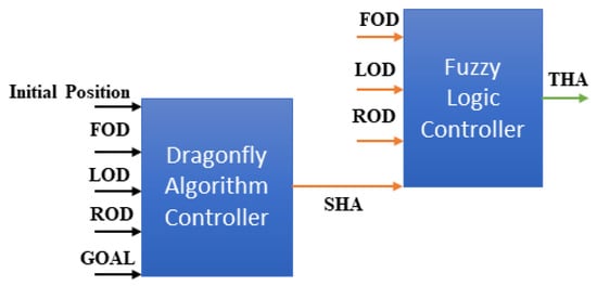
Figure 4.
Dragonfly–fuzzy hybrid controller architecture.
In this study, the autonomous vehicle employs eight sensors distributed around its periphery to detect obstacles and determine the goal’s position, enabling the calculation of key pointers such as front obstacle distance (FOD), left obstacle distance (LOD), and right obstacle distance (ROD). The hybrid controller integrates inputs from the DA controller and obstacle distances to generate the steep heading angle (SHA). The output from the DA controller is utilized to train the fuzzy logic controller, which, in turn, determines the total heading angle (THA), which is applicable to various environmental conditions.
The design incorporates an obstacle avoidance feature to prevent collisions with obstacles in the vehicle’s environment. Emphasis is placed on positioning the food source in the global best position, ensuring it is kept as far away as possible from the nearest obstacle. This strategy aims to optimize the vehicle’s trajectory and enhance obstacle avoidance capabilities. The Euclidean distance between the global best position (food source) and the most immediate environmental obstacle is used to calculate the objective function, given by the Equation (15).
where and are the best position, and and is the position of the closest obstacle. The Euclidean distance between the most relative obstacle and the vehicle is calculated using Equation (16).
The best position for the dragonfly’s food source should be as close to the goal as possible. The target-seeking objective function is defined as the Euclidean distance between the best position and the goal in the environment, given by Equation (17).
where and are the goal position, and is the minimum Euclidean distance from the vehicle to the position of the food source.
The equation defines the objective function of path optimization, which combines obstacle-seeking and target-seeking behavior.
When the vehicle moves in an unstructured environment, it encounter different obstacles, known as . In this objective function, it is clearly specified that when Fi comes closer to the goal, the value will decrease, and when Fi moves far away from the obstacles, the objective function value will be larger. The objective function incorporates parameters denoted as C1 and C2, which are recognized as fitting and controlling parameters, respectively, and it is evident that these parameters significantly impact the trajectory of the vehicle. When C1 is excessively large, the robot tends to maintain a considerable distance from obstacles, whereas overly small values of C1 may lead to collisions with objects in the surroundings. Similarly, a large value of C2 inclines the robot towards a shorter and more optimal path to the target, whereas smaller values result in longer pathways. These control settings play a crucial role in expediting the convergence of the objective function and eliminating local minima. The determination of these control settings in this study involved a trial-and-error approach.
The dragonfly algorithm (DA) controller produces an output that serves as input for the fuzzy logic (FL) controller in the hybrid system. Following this, the FL controller refines the parameters from the DA controller, leading to the determination of the optimal values for the hybrid controller. Fuzzy logic, acknowledged for its universal approximation properties, demonstrates the ability to perform any nonlinear mapping between input sensor data and the central variable output. Linguistic expressions assigned to front obstacle distance (FOD), left obstacle distance (LOD), and right obstacle distance (ROD) encompass terms such as “too close”, “very close”, “close”, “far”, “very far”, and “too far.” Correspondingly, the heading angle utilizes linguistic terms such as “too wide”, “moderately wide”, “wide”, “short”, “moderately short”, and “too short” as outputs. The membership functions employed for these linguistic terms are visually represented in Figure 5. Detailed illustrations of all fuzzy if–then rule mechanisms can be found in Table 1 and Table 2.
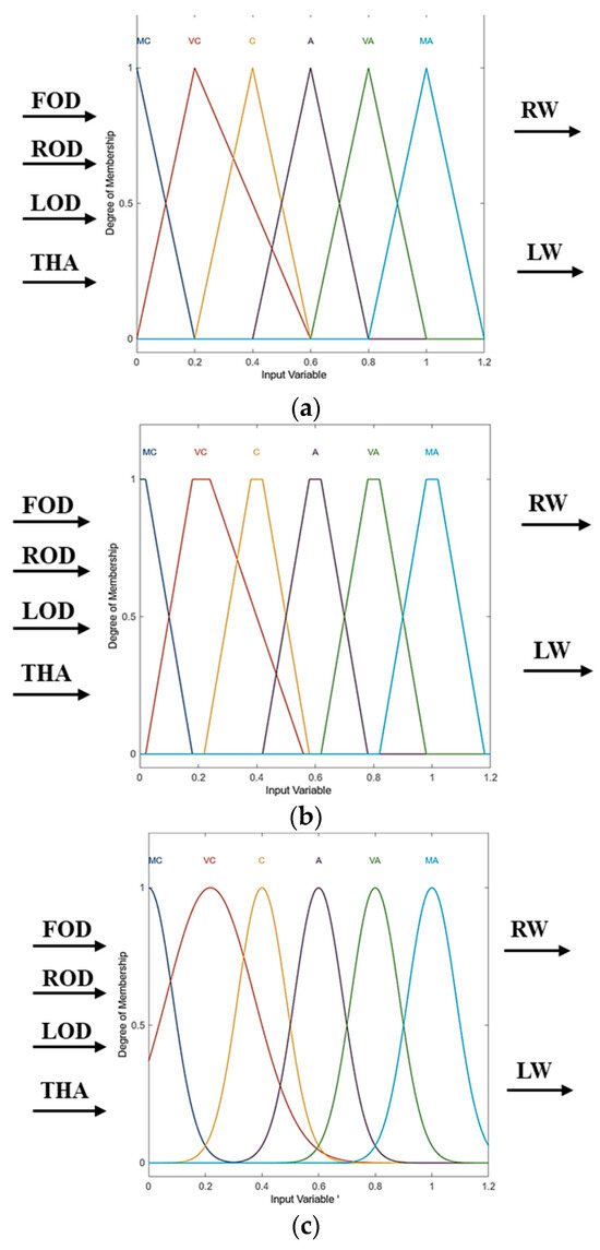
Figure 5.
Fuzzy logic membership functions: (a) triangular; (b) trapezoidal; (c) Gaussian.

Table 1.
FL parameters for obstacles.
Table 2.
FL parameters for heading angle.
Selected fuzzy logic rules for robot navigation:
- If the front obstacle distance (FOD) is negative (N), the left obstacle distance (LOD) is negative (N), and the right obstacle distance (ROD) is positive (F), then the heading angle (HA) is positive, the left velocity (LV) is slow, and the right velocity (RV) is fast.
- If the FOD is medium (M), the LOD is negative (N), and the ROD is positive (F), then the HA is zero, the LV is medium, and the RV is medium.
- If the FOD is positive (F), the LOD is negative (N), and the ROD is positive (F), then the HA is negative, the LV is fast, and the RV is slow.
- If the FOD is negative (N), the LOD is medium (M), and the ROD is positive (F), then the HA is positive, the LV is slow, and the RV is fast.
- If the FOD is medium (M), the LOD is medium (M), and the ROD is positive (F), then the HA is zero, the LV is medium, and the RV is medium.
- If the FOD is positive (F), the LOD is medium (M), and the ROD is positive (F), then the HA is negative, the LV is fast, and the RV is slow.
- If the FOD is negative (N), the LOD is negative (N), and the ROD is negative (N), then the HA is positive, the LV is slow, and the RV is fast.
- If the FOD is medium (M), the LOD is negative (N), and the ROD is negative (N), then the HA is zero, the LV is medium, and the RV is medium.
- If the FOD is positive (F), the LOD is negative (N), and the ROD is negative (N), then the HA is negative, the LV is Fast, and the RV is slow.
- If the FOD is negative (N), the LOD is medium (M), and the ROD is negative (N), then the HA is positive, the LV is slow, and the RV is fast.
4. Experimental and Simulation Results
The presentation of both simulation and experimental outcomes is included herein to authenticate the suggested experimental controller. Utilizing the Fire Bird V robot in this trial, as depicted in Figure 6, enhanced the versatility of the experiment. The Fire Bird V is equipped with an ATMEGA2560 (AVR) microcontroller adaptor board, contributing to its adaptability.
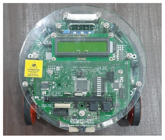
Figure 6.
Fire Bird V robot.
A simulation environment featuring obstacles was employed using the MATLAB R2021a simulation software to assess the efficiency of the suggested controller based on the dragonfly algorithm (DA). The evaluation focused on determining the optimality with respect to both the path length and the time needed for navigation. In order to identify the optimal parameters for the previously described objective function, systematic experiments were carried out involving the variation of multiple controlled parameters, as outlined in Table 3.
Table 3.
Optimal tuning parameters for the DA-based controller.
The computational time was analyzed across different population sizes for the dragonfly algorithm, providing insights into how the algorithm’s performance scaled with the number of individuals in the population. Figure 7 illustrates that the computational time was particularly efficient with a population size of N = 30.
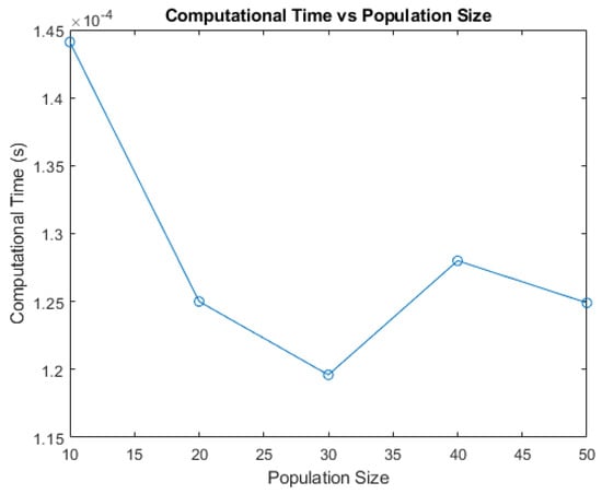
Figure 7.
Population size analysis.
This study showcases the efficacy of our newly devised methodology under a range of environmental circumstances. We performed numerous experiments in settings characterized by static conditions and incorporated diverse obstacles. Utilizing the MATLAB R2021a software for simulation analysis provided us with the capability to tailor the environment by manipulating obstacle locations, robot placements, and objectives. In static scenarios, obstacles were stationary, which permitted modifications solely in the initial positions of the robot and the goal. Our software was configured to adapt to a varying number of robots and goals, thereby ensuring versatility in the experimental setups. The simulation results confirm that the three controllers (DA, FL, DA-FL) were used for navigation in the presence of obstacles represented by green blocks, and the outcome as a navigated path from a red circle representing the start position, while red square representing goal position are depicted in Figure 8, Figure 9 and Figure 10. The path length and the time of the three controllers are shown in Table 4.
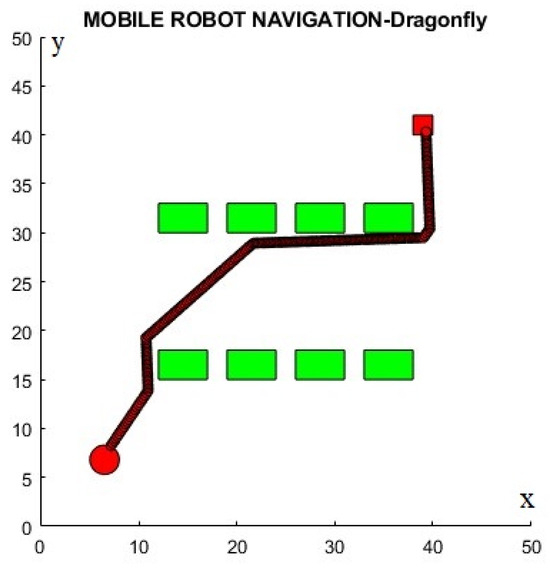
Figure 8.
Navigation using standalone DA.
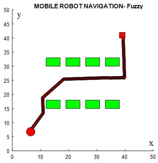
Figure 9.
Navigation using standalone FL.
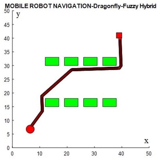
Figure 10.
Navigation using the DA–FL hybrid.
Table 4.
Simulation path length and time of DA, FL, and DA–FL.
All three controllers (DA, FL, DA–FL) were experimentally run in a similar environment to validate the simulation results, as shown in Figure 11, where the movement is shown in four phases from 1–4 and the red dotted line is the path followed by the mobile robot. These experimental results are presented for the path length and navigation time, as shown in Table 5.
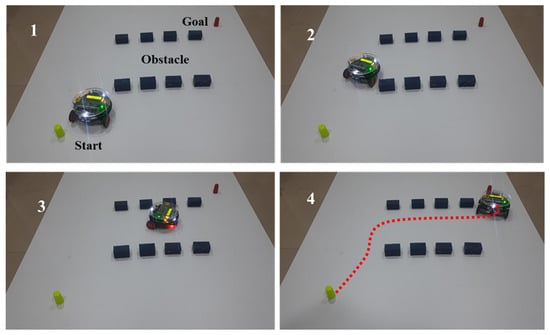
Figure 11.
Experimental setup for mobile robot navigation of all controllers.
Table 5.
Experimental path length and time of DA, FL, and DA–FL.
The proposed dragonfly–fuzzy hybrid controller was compared to existing standalone navigational controllers in the same environmental configuration configuration showcasing phase 4 (reached goal), as shown in Figure 12, to determine its success. Table 6 and Table 7 compare the simulation and experimental results for all three controllers in terms of time and path length.
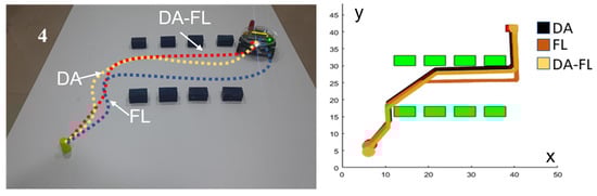
Figure 12.
DA–FL hybrid controller versus another controller.
Table 6.
Path length comparison of DA, FL, and DA–FL.
Table 7.
Navigational time comparison of DA, FL, and DA–FL.
The performance evaluation of the proposed dragonfly–fuzzy controller was meticulously conducted through simulation analysis, enhancing the clarity and transparency in the comparison with two existing controllers under two distinct environmental setups. Figure 13a showcases Joshi and Zaveri’s [43] neuro–fuzzy controller, whereas Figure 14a depicts Patle et al.’s [44] firefly–fuzzy algorithm leveraged for mobile robot navigation in a simulated environment. Correspondingly, Figure 13b and Figure 14b demonstrate that consistent environmental conditions were maintained and detail the number, dimensions, and positions of the obstacles, as well as the initial and final positions of the unmanned vehicle. These enhancements aim to provide comprehensive insight into the scenarios tested.
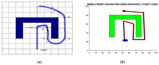
Figure 13.
Comparison of dragonfly–fuzzy algorithm with neuro–fuzzy algorithm: (a) neuro–fuzzy algorithm [43]; (b) dragonfly–fuzzy algorithm.
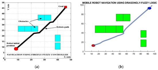
Figure 14.
Comparison of dragonfly–fuzzy algorithm with firefly–fuzzy algorithm: (a) firefly–fuzzy algorithm [44]; (b) dragonfly–fuzzy algorithm.
Upon comparing the performance, the dragonfly–fuzzy controller consistently outperformed both alternatives, achieving path savings of approximately 8.62% against the neuro–fuzzy controller and of around 4.2% against the firefly–fuzzy controller, as detailed in Table 8. This underscores the dragonfly–fuzzy controller’s superior path efficiency in simulated environments, ensuring optimized and effective navigation for unmanned vehicles. The results affirm its proficiency in discovering shorter and more efficient paths while adeptly avoiding unnecessary detours around obstacles. Notably, the controller’s adaptive trajectory optimization for unmanned vehicles positions it as a promising and effective choice for path planning in mobile robot navigation scenarios. The provided systematic contrast analysis, incorporating environmental setups and detailed performance metrics, strengthens the validity and comprehensibility of the evaluation.
Table 8.
Simulation results with other hybrid controllers.
In a comparative study conducted by Xiang et al. [45], the effectiveness of the dragonfly–fuzzy algorithm for mobile robot navigation was assessed against traditional A* and A*–greedy algorithms, as illustrated through the simulation depicted in Figure 15. The results of the comparison detailed in Table 8 reveal notable advantages of the dragonfly–fuzzy algorithm over the conventional A* algorithm. Specifically, it was observed that the dragonfly–fuzzy algorithm achieved a 3.6% reduction in path length compared to the traditional A* algorithm. Additionally, the computational time was significantly reduced, showcasing an 11% improvement. When compared to the A*–greedy algorithm, the dragonfly–fuzzy algorithm demonstrated a similar path length with only minor variations, yet it exhibited significant savings in computational time. These findings underscore the efficiency and effectiveness of the dragonfly fuzzy algorithm in mobile robot navigation, making it a promising alternative for optimizing path planning and reducing computational overhead when compared to traditional A* and A*–greedy approaches.
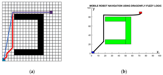
Figure 15.
Comparison of A*–greedy algorithm with dragonfly–fuzzy algorithm: (a) A*–greedy algorithm [45]; (b) dragonfly–fuzzy algorithm.
5. Conclusions
Different standalone metaheuristic algorithms were investigated in this work to solve the navigational problem of an autonomous vehicle, and a new hybrid method was introduced. The proposed DA–FL controller was tested successfully against the standalone DA and FL controllers in a static obstacle environment. A set of experiments was performed to adjust the autonomous vehicle’s parameters, which are directly connected to the smoothness of the generated path. The suggested technique allowed the autonomous vehicle to reach its destination while avoiding obstacles and following a significantly optimized path. Experimental and simulation findings demonstrate that the variation percentage was around 4% to 5% with the optimum path and time. When comparing the proposed hybrid controller and the standalone controller, it was found that the DA–FL hybrid controller took the shortest path and time. Also, the simulation was compared with other results by creating the same environment, and it was found that the dragonfly–fuzzy controller outperformed in terms of saving path length and time. In the future, the dragonfly–fuzzy controller can be implemented in a dynamic environment. It can be tested for navigation for underwater robots and aerial vehicles.
Author Contributions
Conceptualization and supervision, B.P. and S.B.; methodology and validation, B.P. and N.S.; software and investigation, V.D.; writing—original draft preparation, B.P. and V.D. All authors have read and agreed to the published version of the manuscript.
Funding
This research received no external funding.
Institutional Review Board Statement
Not applicable.
Informed Consent Statement
Not applicable.
Data Availability Statement
The data presented in this study are available on request from the corresponding author. The data are not publicly available due to privacy.
Acknowledgments
The support from the UAV and the Robotics Laboratory of the School of Engineering and IT, MATS University, is appreciated.
Conflicts of Interest
The authors declare no conflicts of interest.
References
- Oleari, F.; Magnani, M.; Ronzoni, D.; Sabattini, L. Industrial AGVs: Toward a pervasive diffusion in modern factory warehouses. In Proceedings of the 2014 IEEE 10th International Conference on Intelligent Computer Communication and Processing (ICCP), Cluj-Napoca, Romania, 4–6 September 2014; pp. 233–238. [Google Scholar]
- Monios, J.; Bergqvist, R. Logistics and the networked society: A conceptual framework for smart network business models using electric autonomous vehicles (EAVs). Technol. Forecast. Soc. Chang. 2020, 151, 119824. [Google Scholar] [CrossRef]
- Nakhaeinia, D.; Tang, S.H.; Noor, S.M.; Motlagh, O. A review of control architectures for autonomous navigation of mobile robots. Int. J. Phys. Sci. 2011, 6, 169–174. [Google Scholar]
- Sudhakara, P.; Ganapathy, V.; Priyadharshini, B.; Sundaran, K. Obstacle avoidance and navigation planning of a wheeled mobile robot using amended artificial potential field method. Procedia Comput. Sci. 2018, 133, 998–1004. [Google Scholar] [CrossRef]
- Yazici, A.; Kirlik, G.; Parlaktuna, O.; Sipahioglu, A. A dynamic path planning approach for multirobot sensor-based coverage considering energy constraints. IEEE Trans. Cybern. 2013, 44, 305–314. [Google Scholar] [CrossRef]
- Patle, B.; Patel, B.; Jha, A. Rule-Based Fuzzy Decision Path Planning Approach for Mobile Robot. In Proceedings of the 2018 Fourth International Conference on Computing Communication Control and Automation (ICCUBEA), Pune, India, 16–18 August 2018; pp. 1–7. [Google Scholar]
- Hart, P.E.; Nilsson, N.J.; Raphael, B. A formal basis for the heuristic determination of minimum cost paths. IEEE Trans. Syst. Sci. Cybern. 1968, 4, 100–107. [Google Scholar] [CrossRef]
- Karaman, S.; Walter, M.R.; Perez, A.; Frazzoli, E.; Teller, S. Anytime motion planning using the RRT. In Proceedings of the 2011 IEEE International Conference on Robotics and Automation, Shanghai, China, 9–13 May 2011; pp. 1478–1483. [Google Scholar]
- Hauer, F.; Tsiotras, P. Deformable Rapidly-Exploring Random Trees. In Proceedings of the Robotics: Science and Systems, Cambridge, MA, USA, 12–16 July 2017. [Google Scholar]
- Kavraki, L.; Latombe, J. Probabilistic roadmaps for robot path planning. In Pratical Motion Planning in Robotics: Current Aproaches and Future Challenges; Wiley: Hoboken, NJ, USA, 1998; pp. 33–53. [Google Scholar]
- Sun, Z.; Wu, J.; Yang, J.; Huang, Y.; Li, C.; Li, D. Path planning for GEO-UAV bistatic SAR using constrained adaptive multiobjective differential evolution. IEEE Trans. Geosci. Remote Sens. 2016, 54, 6444–6457. [Google Scholar] [CrossRef]
- Dujari, R.; Patel, B.; Patle, B. Adaptive Mayfly Algorithm for UAV Path Planning and Obstacle Avoidance in Indoor Environment. In Proceedings of the 2023 International Conference on Network, Multimedia and Information Technology (NMITCON), Bengaluru, India, 1–2 September 2023; pp. 1–7. [Google Scholar]
- Yi, X.; Zhu, A.; Yang, S. MPPTM: A Bio-Inspired Approach for Online Path Planning and High-Accuracy Tracking of UAVs. Front. Neurorobot. 2022, 15, 798428. [Google Scholar] [CrossRef] [PubMed]
- Ganapathy, V.; Sudhakara, P.; Jie, T.J.; Parasuraman, S. Mobile robot navigation using amended ant colony optimization algorithm. Indian J. Sci. Technol. 2016, 9, 1–10. [Google Scholar] [CrossRef]
- Xin, J.; Li, S.; Sheng, J.; Zhang, Y.; Cui, Y. Application of improved particle swarm optimization for navigation of unmanned surface vehicles. Sensors 2019, 19, 3096. [Google Scholar] [CrossRef] [PubMed]
- Patel, B.; Patle, B. Analysis of firefly–fuzzy hybrid algorithm for navigation of quad-rotor unmanned aerial vehicle. Inventions 2020, 5, 48. [Google Scholar] [CrossRef]
- Xing, B.; Gao, W.-J.; Xing, B.; Gao, W.-J. Fruit fly optimization algorithm. In Innovative Computational Intelligence: A Rough Guide to 134 Clever Algorithms; Springer: Cham, Switzerland, 2014; pp. 167–170. [Google Scholar]
- Wang, G.-G.; Chu, H.E.; Mirjalili, S. Three-dimensional path planning for UCAV using an improved bat algorithm. Aerosp. Sci. Technol. 2016, 49, 231–238. [Google Scholar] [CrossRef]
- Liu, J.; Wei, X.; Huang, H. An improved grey wolf optimization algorithm and its application in path planning. IEEE Access 2021, 9, 121944–121956. [Google Scholar] [CrossRef]
- Meraihi, Y.; Gabis, A.B.; Mirjalili, S.; Ramdane-Cherif, A. Grasshopper optimization algorithm: Theory, variants, and applications. IEEE Access 2021, 9, 50001–50024. [Google Scholar] [CrossRef]
- Guruji, A.K.; Agarwal, H.; Parsediya, D. Time-efficient A* algorithm for robot path planning. Procedia Technol. 2016, 23, 144–149. [Google Scholar] [CrossRef]
- Antonelli, G.; Chiaverini, S.; Fusco, G. A fuzzy-logic-based approach for mobile robot path tracking. IEEE Trans. Fuzzy Syst. 2007, 15, 211–221. [Google Scholar] [CrossRef]
- Dubey, V.; Barde, S.; Patel, B. Obstacle Finding and Path Planning of Unmanned Vehicle by Hybrid Techniques. In Information Systems and Management Science, Proceedings of the 4th International Conference on Information Systems and Management Science (ISMS) 2021, Msida, Malta, 14–15 December 2021; Springer: Cham, Switzerland, 2022; pp. 28–36. [Google Scholar]
- Kanoon, Z.E.; Araji, A.; Abdullah, M.N. Enhancement of Cell Decomposition Path-Planning Algorithm for Autonomous Mobile Robot Based on an Intelligent Hybrid Optimization Method. Int. J. Intell. Eng. Syst. 2022, 15, 161–175. [Google Scholar]
- Murofushi, T.; Sugeno, M. Fuzzy control of model car. J. Robot. Soc. Jpn. 1988, 6, 536–541. [Google Scholar] [CrossRef][Green Version]
- Langari, R. Past, present and future of fuzzy control: A case for application of fuzzy logic in hierarchical control. In Proceedings of the 18th International Conference of the North American Fuzzy Information Processing Society-NAFIPS (Cat. No. 99TH8397), New York, NY, USA, 10–12 June 1999; pp. 760–765. [Google Scholar]
- Berisha, J.; Bajrami, X.; Shala, A.; Likaj, R. Application of Fuzzy Logic Controller for obstacle detection and avoidance on real autonomous mobile robot. In Proceedings of the 2016 5th Mediterranean Conference on Embedded Computing (MECO), Bar, Montenegro, 12–16 June 2016; pp. 200–205. [Google Scholar]
- Fernando, T.; Gammulle, H.; Walgampaya, C. Fuzzy logic based mobile robot target tracking in dynamic hostile environment. In Proceedings of the 2015 IEEE International Conference on Computational Intelligence and Virtual Environments for Measurement Systems and Applications (CIVEMSA), Shenzhen, China, 12–14 June 2015; pp. 1–6. [Google Scholar]
- Mirjalili, S. Dragonfly algorithm: A new meta-heuristic optimization technique for solving single-objective, discrete, and multi-objective problems. Neural Comput. Appl. 2016, 27, 1053–1073. [Google Scholar] [CrossRef]
- Abdel-Basset, M.; Luo, Q.; Miao, F.; Zhou, Y. Solving 0–1 knapsack problems by binary dragonfly algorithm. In Intelligent Computing Methodologies, Proceedings of the 13th International Conference, ICIC 2017, Liverpool, UK, 7–10 August 2017; Proceedings, Part III 13; Springer: Cham, Switzerland, 2017; pp. 491–502. [Google Scholar]
- Sawhney, R.; Jain, R. Modified binary dragonfly algorithm for feature selection in human papillomavirus-mediated disease treatment. In Proceedings of the 2018 International Conference on Communication, Computing and Internet of Things (IC3IoT), Chennai, India, 15–17 February 2018; pp. 91–95. [Google Scholar]
- Mafarja, M.; Aljarah, I.; Heidari, A.A.; Faris, H.; Fournier-Viger, P.; Li, X.; Mirjalili, S. Binary dragonfly optimization for feature selection using time-varying transfer functions. Knowl.-Based Syst. 2018, 161, 185–204. [Google Scholar] [CrossRef]
- Abuomar, L.; Al-Aubidy, K. Cooperative search and rescue with swarm of robots using binary dragonfly algoritlnn. In Proceedings of the 2018 15th International Multi-Conference on Systems, Signals & Devices (SSD), Yassmine Hammamet, Tunisia, 19–22 March 2018; pp. 653–659. [Google Scholar]
- Sayed, G.I.; Tharwat, A.; Hassanien, A.E. Chaotic dragonfly algorithm: An improved metaheuristic algorithm for feature selection. Appl. Intell. 2019, 49, 188–205. [Google Scholar] [CrossRef]
- Sambandam, R.K.; Jayaraman, S. Self-adaptive dragonfly based optimal thresholding for multilevel segmentation of digital images. J. King Saud Univ.-Comput. Inf. Sci. 2018, 30, 449–461. [Google Scholar] [CrossRef]
- Ji, J.; Khajepour, A.; Melek, W.W.; Huang, Y. Path planning and tracking for vehicle collision avoidance based on model predictive control with multiconstraints. IEEE Trans. Veh. Technol. 2016, 66, 952–964. [Google Scholar] [CrossRef]
- Viadero-Monasterio, F.; Nguyen, A.-T.; Lauber, J.; Boada, M.J.L.; Boada, B.L. Event-triggered robust path tracking control considering roll stability under network-induced delays for autonomous vehicles. IEEE Trans. Intell. Transp. Syst. 2023. [Google Scholar] [CrossRef]
- Xu, S.; Peng, H. Design, analysis, and experiments of preview path tracking control for autonomous vehicles. IEEE Trans. Intell. Transp. Syst. 2019, 21, 48–58. [Google Scholar] [CrossRef]
- Hu, C.; Wang, R.; Yan, F.; Chen, N. Output constraint control on path following of four-wheel independently actuated autonomous ground vehicles. IEEE Trans. Veh. Technol. 2015, 65, 4033–4043. [Google Scholar] [CrossRef]
- Chen, T.; Chen, L.; Xu, X.; Cai, Y.; Sun, X. Simultaneous path following and lateral stability control of 4WD-4WS autonomous electric vehicles with actuator saturation. Adv. Eng. Softw. 2019, 128, 46–54. [Google Scholar] [CrossRef]
- Kennedy, J.; Eberhart, R. Particle swarm optimization. In Proceedings of the ICNN’95—International Conference on Neural Networks, Perth, WA, Australia, 27 November–1 December 1995; pp. 1942–1948. [Google Scholar]
- Zadeh, L.A. Fuzzy sets. Inf. Control 1965, 8, 338–353. [Google Scholar] [CrossRef]
- Joshi, M.M.; Zaveri, M.A. Reactive navigation of autonomous mobile robot using neuro-fuzzy system. Int. J. Robot. Autom. (IJRA) 2011, 2, 128. [Google Scholar]
- Patle, B.; Patel, B.; Pandey, A.; Sahu, O.; Parhi, D. Analysis of Firefly-Fuzzy Hybrid Controller for Wheeled Mobile Robot. In Proceedings of the 2019 3rd International Conference on Computing and Communications Technologies (ICCCT), Chennai, India, 21–22 February 2019; pp. 187–194. [Google Scholar]
- Xiang, D.; Lin, H.; Ouyang, J.; Huang, D. Combined improved A* and greedy algorithm for path planning of multi-objective mobile robot. Sci. Rep. 2022, 12, 13273. [Google Scholar] [CrossRef] [PubMed]
Disclaimer/Publisher’s Note: The statements, opinions and data contained in all publications are solely those of the individual author(s) and contributor(s) and not of MDPI and/or the editor(s). MDPI and/or the editor(s) disclaim responsibility for any injury to people or property resulting from any ideas, methods, instructions or products referred to in the content. |
© 2024 by the authors. Licensee MDPI, Basel, Switzerland. This article is an open access article distributed under the terms and conditions of the Creative Commons Attribution (CC BY) license (https://creativecommons.org/licenses/by/4.0/).