Article

Sliding Mode Control for Single-Phase Grid-Connected Voltage Source Inverter with L and LCL Filters

by
Moacyr A. G. de Brito
1,*,
Egon H. B. Dourado
1,
Leonardo P. Sampaio
2,
Sergio A. O. da Silva
2 and
Raymundo C. Garcia
1
1
Electrical Engineering Department, Faculty of Engineering, Architecture and Urbanism and Geography, Federal University of Mato Grosso do Sul—UFMS, Campo Grande 79070-900, MS, Brazil
2
Electrical Engineering Department, Federal Technological University of Paraná—UTFPR, Cornélio Procópio 86300-000, PR, Brazil
*
Author to whom correspondence should be addressed.
Eng 2023, 4(1), 301-316; https://doi.org/10.3390/eng4010018
Submission received: 18 December 2022 / Revised: 11 January 2023 / Accepted: 18 January 2023 / Published: 20 January 2023
(This article belongs to the Section Electrical and Electronic Engineering)

Abstract

:
This paper presents an analysis of the sliding mode control (SMC) method applied to a single-phase grid-connected voltage source inverter (VSI) with L and LCL filters. First, simulation results were presented for the L filter, and then, after some adjustments, the same theory was applied to the LCL VSI with active damping. To improve the obtained results for the SMC control, we adopted the hyperbolic tangent function and the explicit establishment of the modulation index m in the mathematical procedure to help reduce the chattering phenomena; later on, the same function was replaced by the usage of a proportional plus resonant controller to continuously improve the control system responses.

1. Introduction

Because of the continuous search for improvements in energy systems (generation, management, and consumption) focused on alternative and renewable energy sources, growth in the distributed generation market has been noted worldwide. The perspective is changing rapidly due to three of humanity’s great concerns, which are increasingly present today: the environment, energy, and the global economy [1].
The annual global energy market, more specifically for the photovoltaic panels (PVs), showed a small increase in 2018, but this was enough to exceed 100 GW (including the on-grid and off-grid installed capacity) for the first time [2]. Despite its low growth rate in 2018, photovoltaic energy has become one of the fastest-growing energy sources in the world, with gigawatt-scale markets in an increasing number of countries, especially in the year 2022, exceeding 300 GW [3]. Some important characteristics of PV systems are the inherent scalability property; regarding solar energy, they are also pollution-free and abundant, and they participate as a primary factor of all other processes of energy production on Earth [4].
Considering the growing interest in renewable sources, the system connection, which comprises the integration of an inverter to the grid, must be safely executed. Such need encouraged the emergence of several areas of research; among these, it is relevant to highlight the schemes of stabilization control since the control of these systems must achieve high performance, characterized by a fast dynamic response, robustness to disturbances, null tracking error, and low total harmonic distortion (THD) [5].
Many power inverters, through semiconductor device realization, utilize pulse width modulation (PWM) schemes to synthesize the waveforms of interest. However, due to the switching nature, a portion of harmonic content is generated. Considering the typical switching values found in inverters, these can produce harmonics of higher orders that interfere with other loads or sensitive equipment on the grid and can produce losses when circulating in the distribution grid. To deal with this harmonic content, it is common to find filters (such as L or LCL) at the inverter output before actually connecting them to the grid [6,7]. To reduce harmonics and improve the quality of the grid current, filters that consist of an inductive output, such as L or LCL, show favorable characteristics to achieve these objectives. Compared with the L filter, the LCL filter offers greater harmonic attenuation at the same switching frequency with a reduced total filter volume. Although these improvements are attractive, a third-order transfer function for the control of the output current of the LCL filter is created, and due to the interaction between the reactive elements, a peak resonance problem is inserted in the system, which can be reduced by passive or active damping techniques. For low-power inverters, the L filter tends to produce a cost-effective solution [8,9].
In addition to converting energy in the form of direct current (DC) to alternating current (AC), inverters also seek to control power flow and power factor optimization. This is accomplished by several control schemes, such as hysteresis-based strategies, PI (proportional–integral) controller, P + R (proportional–resonant) controller, sliding mode control (SMC), predictive control, deadbeat control, and adaptive control, among others [10].
Since the 1950s, with the work started by Emelyanov and several other researchers, SMC and variable structure control have been widely used and discussed. In variable structure systems, the control law is allowed to alternate at any time among possible continuous functions of a given set, thereby changing the system structure [11,12,13]. The concept of the equivalent control law u s m c , attributed to Utkin, can be written as (1):
u s m c = u e q + δ u
where u e q is the equivalent control law and δ u is the discontinuous portion.
The design of the equivalent control law is obtained after choosing a sliding surface, namely s t , where the dynamics of the states that rule the behavior of a given system must be limited to that surface. For the sliding mode to occur, it is necessary that s t = s ˙ t = 0 . To ensure that the sliding surface is achieved in a finite time, a more restrictive condition must be satisfied. Therefore, a new concept known as the reaching mode is identified, which describes how the controlled states will reach the sliding surface under certain conditions called reach conditions [14].
One of the most used strategies to reach those conditions is known as the reaching law approach, which describes the dynamics for a given switching function f s t [14], as described by (2):
s ˙ t = ε · s i g n s t q · f s t
in which ε and q are restrictively positive constants. Different values for such constants can achieve different behaviors for the reaching law. Increasing q reduces the reaching time, while decreasing ε also decreases the chattering effect.
From the point of view of switching systems, the chattering phenomenon is undesirable in real systems because, in practice, high-speed switching causes reduced equipment life and increased electromagnetic interference; in addition, it is able to excite fast modes of the system that were neglected during the modeling stage, making the system unstable [12,13,14].
For a constant plus proportional reaching rate, (2) is rewritten as (3), and this permits the sliding surface to be used directly to control the power converter, i.e., through its own function and its sign.
s ˙ t = ε · s i g n s t q · s t
In this context, this paper’s proposal was to evaluate the predominant characteristics of the sliding mode control and apply a modified version on a voltage source inverter (VSI) with L and LCL filters. The presented results ensure reference tracking capability with minimal error and low total harmonic distortion (THD) with changes in the traditional SMC method by explicitly finding the inverter modulation index m and, consequently, improving its response with complementary control strategies.

2. System Description

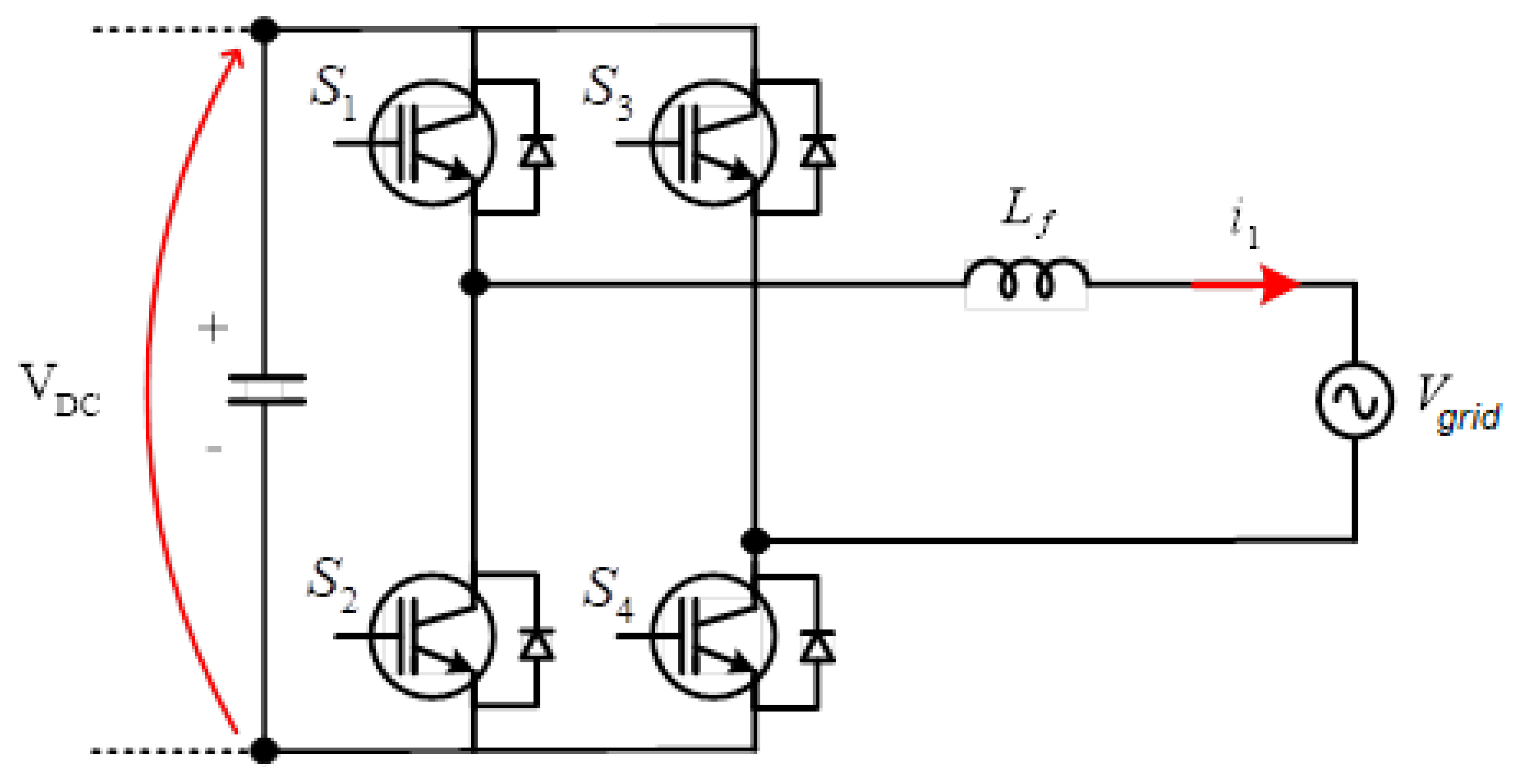
2.1. VSI Plus L Filter

Starting with the VSI with the L filter, represented in Figure 1, some hypotheses should be considered to help simplify the analysis [8]. Thus, at the point of common coupling, the synchronism between the inverter and the grid is already guaranteed by a phase-locked loop algorithm—p-PLL [15]. The switches used by the inverter are considered ideal; despite the predominantly inductive characteristic of the electrical grid, which is disregarded, the grid is modeled as a sinusoidal voltage source V g r i d . The L filter is high enough to attenuate high-order switching effects.
In this paper, the synthesized voltage after the switching bridge is considered to be of m V D C value, where m represents the modulation index, which is the peak value of the sinusoid that controls the switching. In such an approach, the mathematical model can be carried out by explicating this variable to reduce the chattering phenomena. Among the modulation techniques [16], unipolar modulation was chosen, in which three different voltage levels were created by the inverter switching scheme, including + V D C , V D C and 0 .
Kirchhoff’s voltage law was used to describe the dynamics of the system, as seen in (4).
m V D C L f d i 1 d t V g r i d = 0
In order to design the L f filter inductance, it was possible to make use of the current ripple, that is, a maximum current ripple was considered at the grid voltage peak [9]. Thus, (5) describes the obtainment of the L filter. Equation (5) was obtained with some algebraic modifications using Δ v = L f Δ I Δ T ; Δ v represents the voltage in the L f filter, and Δ T is m / f s :
L f = V D C V g r i d P   m f s I 1 Δ I 1
in which f s is the switching frequency, I 1 is the grid current peak, Δ I 1 is the grid current ripple in %, V g r i d P is the grid voltage peak, and m = V g r i d P / V D C .
The main parameters for the design of the L filter are displayed in Table 1. Replacing those values in (5), the value of the filter inductance L f can be found to be approximately 5 mH.
There are different ways to define a sliding surface. One option is to define it as the tracking error, in other words, the difference between the measured variable, grid current, i 1 ( t ), and its reference i 1 * ( t ). In this instance, a zero-order sliding surface is used, as described by (6):
s t = i 1 t i 1 * t = 0
As we are using the concept of the equivalent control law, the time derivative of (6) is written as (7):
s ˙ t = i 1 ˙ t i 1 * ˙ t = 0
From (4), it is found that:
d i 1 d t = m V D C V g r i d L f
Assuming that the reference i 1 * t is of the sinusoidal form and is in phase with the grid voltage employing a PLL, we can write (9):
i 1 * t = I 1 sin ω t
where I 1 is the peak of the reference current.
The time derivative of (9) results in (10).
d i 1 * d t = i 1 * ˙ t = I 1   ω   cos ω t
Substituting (8) into (7) yields:
m V D C V g r i d L f i 1 * ˙ t = 0
After that, (11) is organized to highlight the modulation index m in order to reduce the chattering effect, as described by (12):
m = i 1 * ˙ t + V g r i d V D C
Since the modulation index m is the control variable of the system, i.e., the equivalent control law in steady-state, it is possible to make u e q = m . Thus, (12) represents the equivalent control law. To find the discontinuous portion δ u , the constant plus proportional rate reaching law (3) was used. The ending control law is written as (13):
u s m c = i 1 * ˙ t + V g r i d V D C + δ u
where δ u = ε · s i g n s t q · s t .

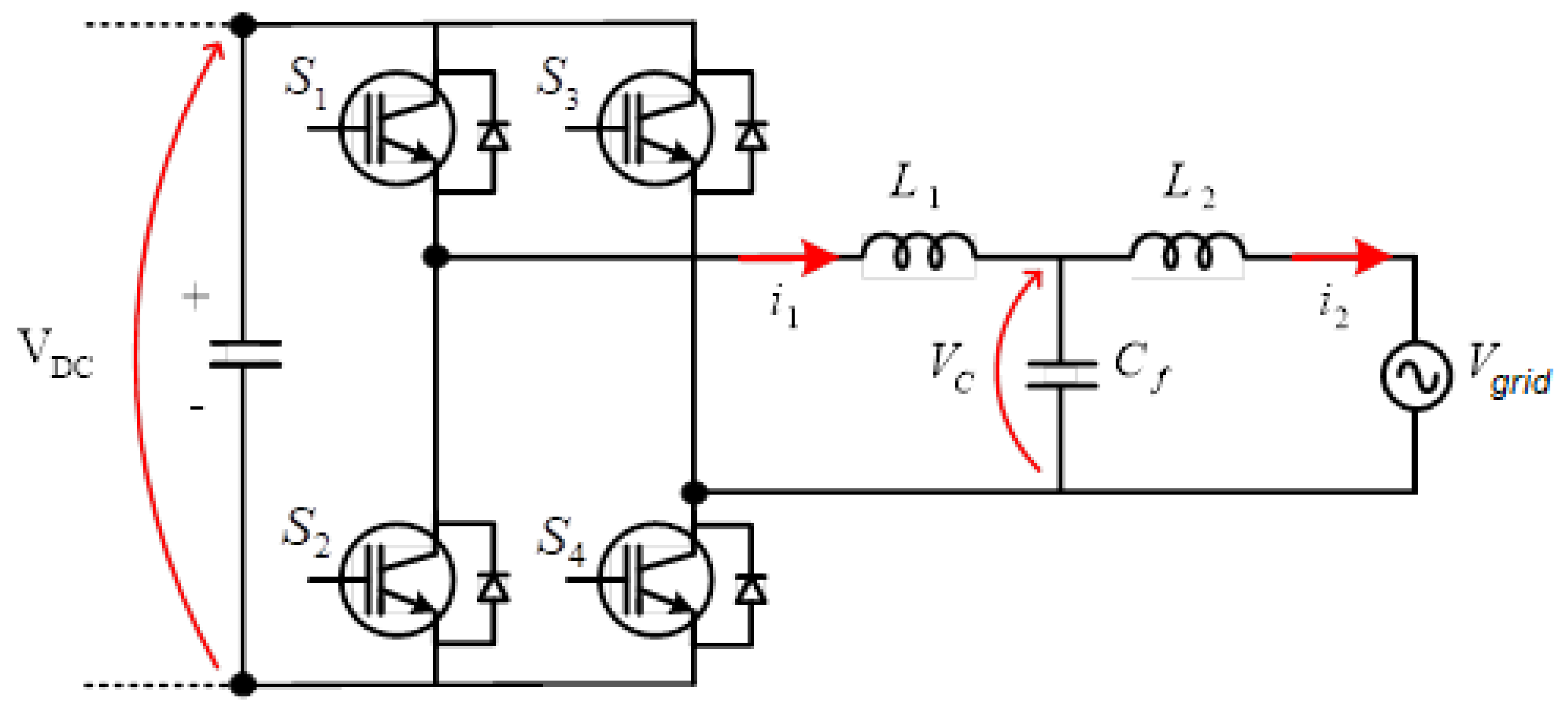
2.2. VSI Plus LCL Filter

Similar to the previous procedures, the sliding mode control method was designed for the LCL filter, but before that, the specifications of the components of the filter were calculated. First, the following limitations were established [7]:
  • The value of the capacitance is limited by the decrease in the power factor that occurs at rated power (usually lower than 5% [17]);
  • The total value of the inductance must be less than 0.1 p.u. to limit the voltage drop during operation. Otherwise, a higher value of DC voltage is required to guarantee the current controllability, resulting in more losses in the system;
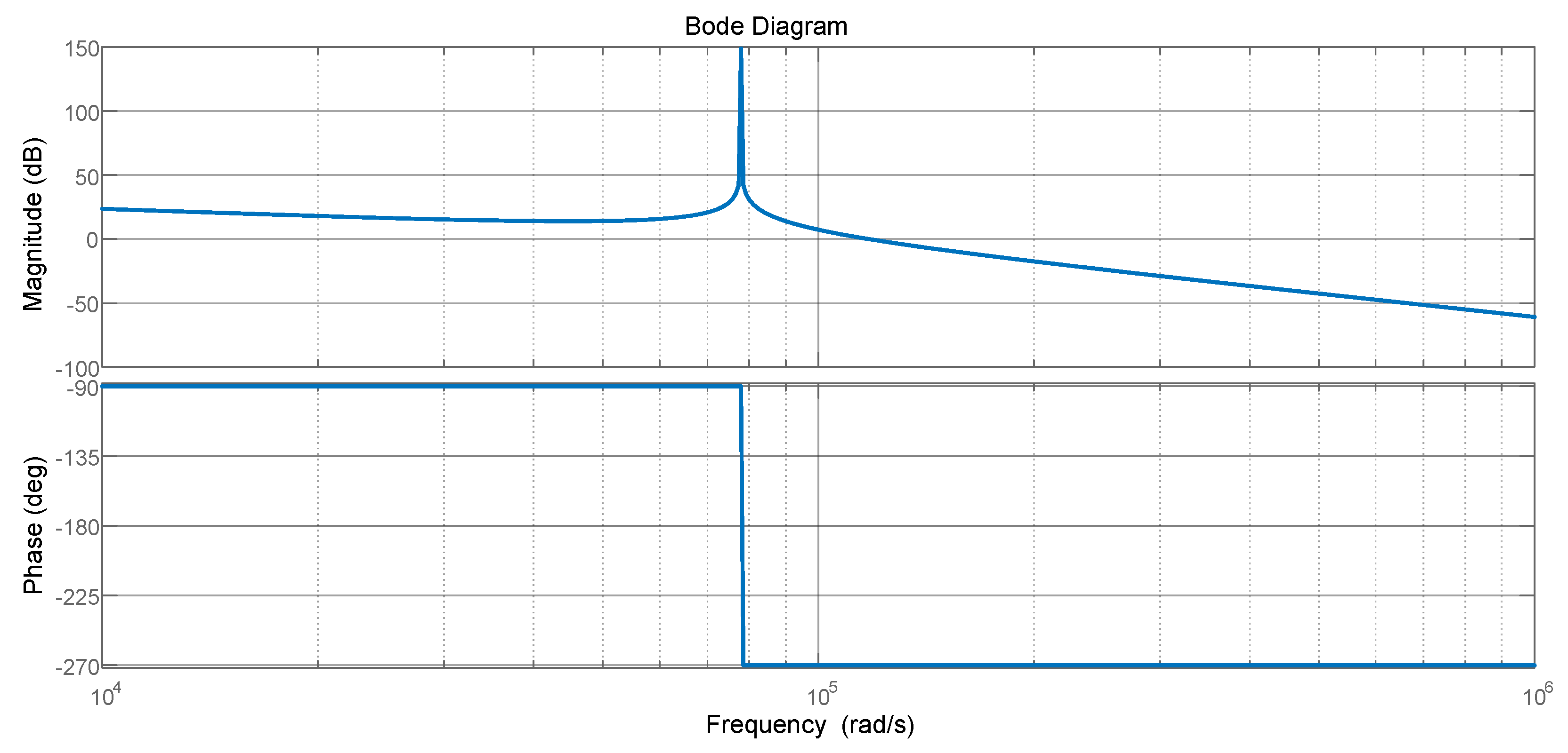
  • To avoid resonance problems among the lower and higher portions of the harmonic spectrum, the resonance frequency f r e s must be in the following range (14), concerning the grid frequency f g and the switching frequency f s [7]:
    10 f g < f r e s < 1 2 f s
Obeying constraint (14) guarantees the proper reduction in the switching harmonics without increasing the phase displacement between the grid voltage and current at the fundamental frequency and the mitigation of resonances.
Considering the aforementioned constraints together with the specifications of the Table 1 parameters, using the methodology presented in [7], it was possible to design the components of the LCL filter. The resulting components are displayed in Table 2.
The circuit represented in Figure 2 is used to describe the dynamics of the system through, once again, Kirchhoff’s laws, as performed previously for the L filter.
The equations that describe the system dynamics are shown in (15) and (16).
L 1 d i 1 d t = m V D C V C
L 2 d i 2 d t = V C V g r i d
The transfer function G m s for the Figure 2 circuit, which relates the grid current i 2 s with the modulation index m , is given by (17).
G m s = i 2 s m s = V D C L 1 L 2 C s 3 + L 1 + L 2 s
However, it is important to note the necessity of employing an active damping technique to suppress the inherent resonance effect of the LCL filter, considering a lossless solution [8,9]. Figure 3 shows the Bode diagram of the designed filter using (17) to exemplify the resonance peak. Observing the diagrams of magnitude (dB) and phase (degrees), one can verify a magnitude of almost 150 dB at the frequency of resonance; this shows the high difficulty of stabilizing this system, thus proving the necessity of damping.
Considering the active damping through the concept of a virtual resistance by the feedback of the capacitor current multiplied by a proportional gain K, the previous transfer function (17) can be rewritten as (18) [18]. The diagram in Figure 4 was used to derive (18) together with the concepts of block diagram reduction [19,20]. For block diagram reduction, v g r i d is considered a disturbance, and, hence, it has a null value. The derivation of (18) can be seen in Appendix A.
G m s = V D C L 1 L 2 C s 3 + K L 2 C s 2 + L 1 + L 2 s
Using the methodology presented in [18] and with a damping coefficient ξ of 1.25, we found the proportional gain K to be 321.63. The damped Bode diagram is depicted in Figure 5, demonstrating the resonance peak mitigation. The K value was chosen to completely remove the peak of resonance, as observed in Figure 5.
Using a similar sliding surface, which was defined by the tracking error of the grid current i 2 , the sliding mode control surface was obtained by (19).
s t = i 2 t i 2 * t = 0
The time derivative of (19) results in (20).
s ˙ t = i 2 ˙ t i 2 * ˙ t = 0
Assuming that the reference current i 2 * has the form of a sinusoidal function (21).
i 2 * t = I 2   sin ω t
where I 2 is the grid current reference peak.
The time derivative of (21) can be written as (22).
i 2 * ˙ t = I 2   ω   c o s ω t
Through (16), i 2 t is described as:
d i 2 d t = V C V g r i d L 2
By isolating V C in (15) and replacing the newly found expression in (23), we obtain (24).
d i 2 d t = m V D C L 1 d i 1 d t V g r i d L 2
It is now possible to turn the modulation index m into the control variable once more, which means that u e q = m , as described by (25). i 2 * ˙ equals d i 2 * d t only for notation simplicity.
m = L 1 d i 1 d t + V g r i d + L 2 i 2 * ˙ V D C
Substituting (24) into (20), the equivalent control law is given by (26):
u s m c = L 1 d i 1 d t + V g r i d + L 2 i 2 * ˙ V D C + δ u
where δ u = ε · s i g n s t q · s t .

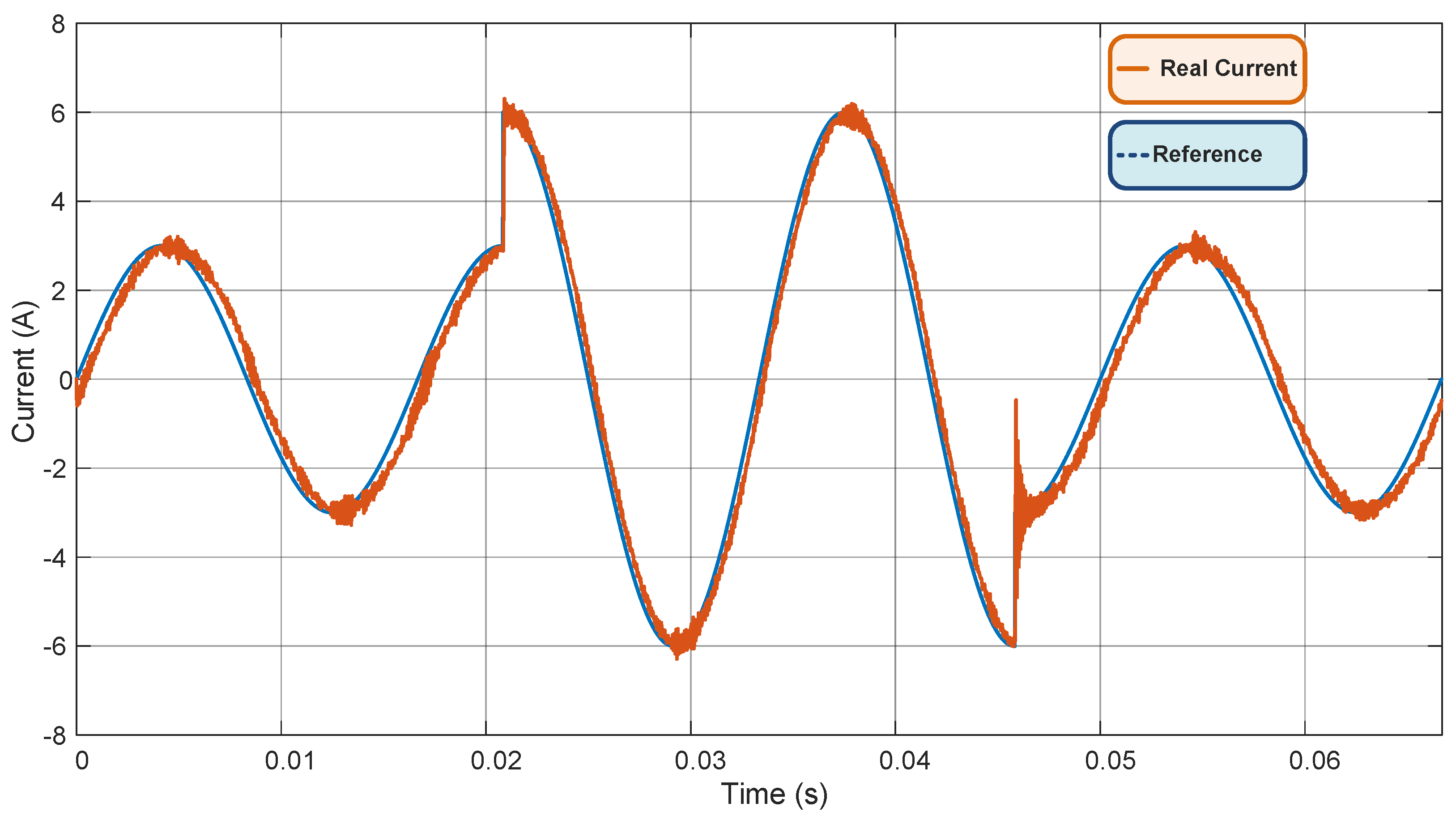
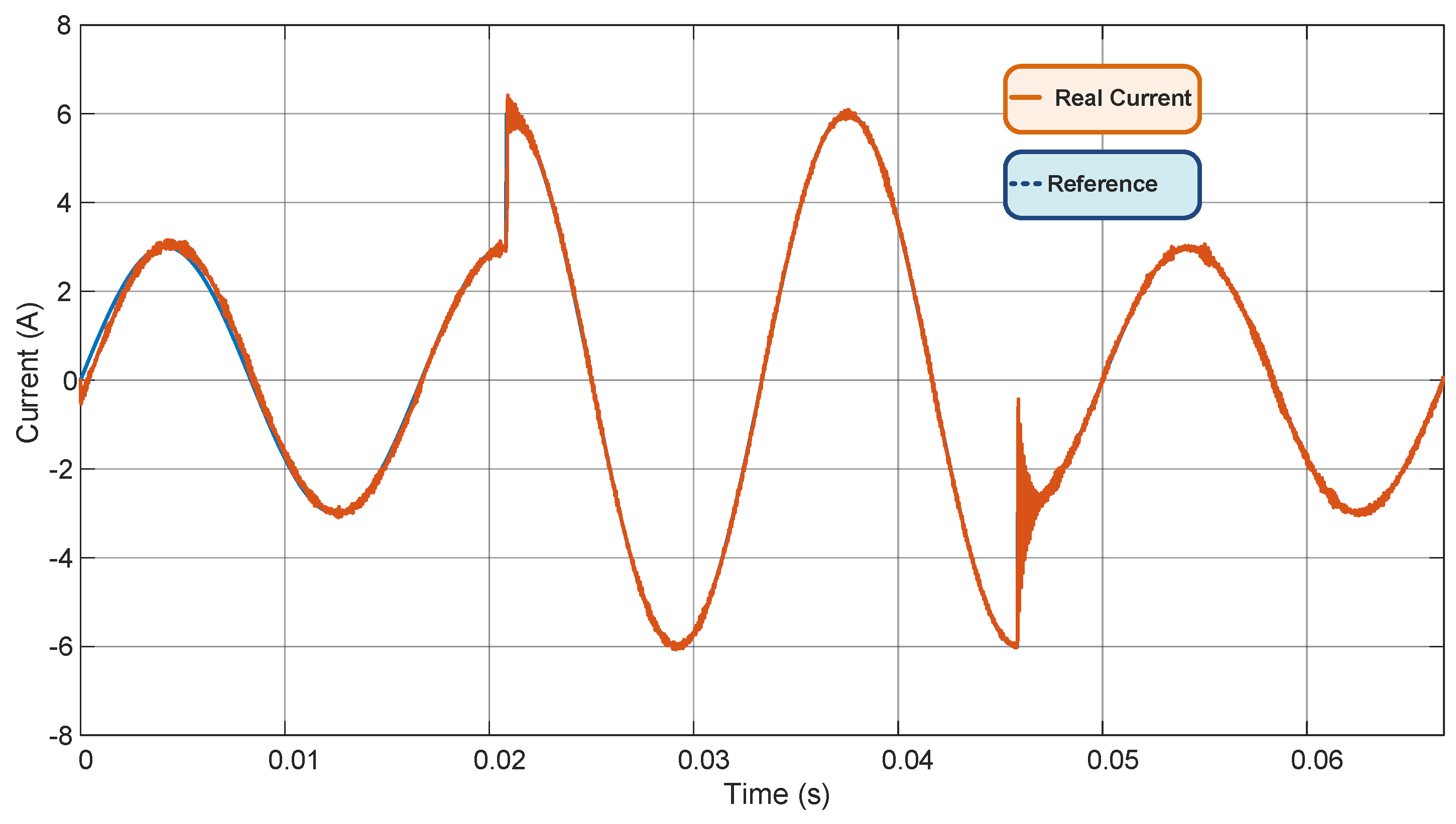
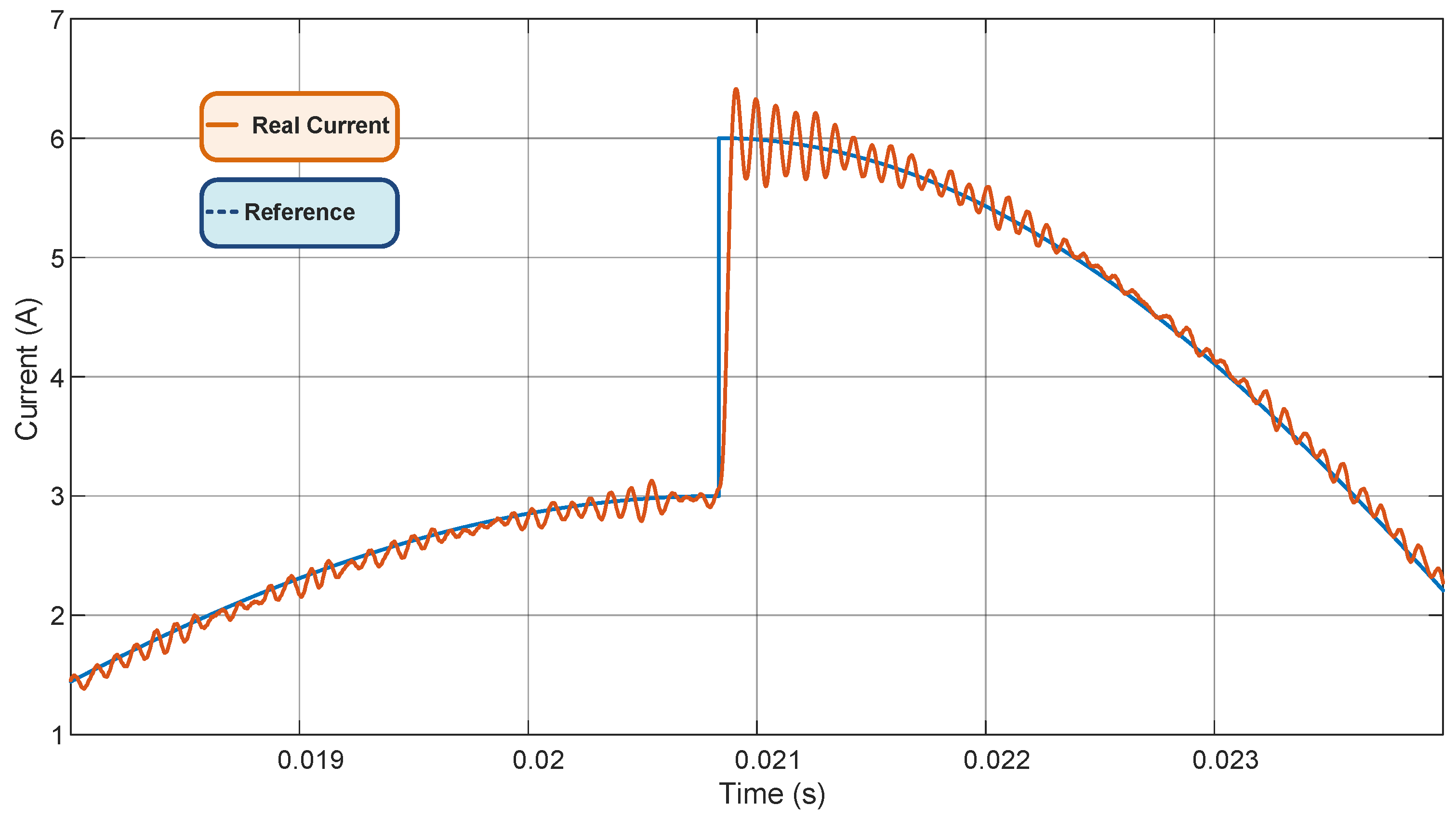
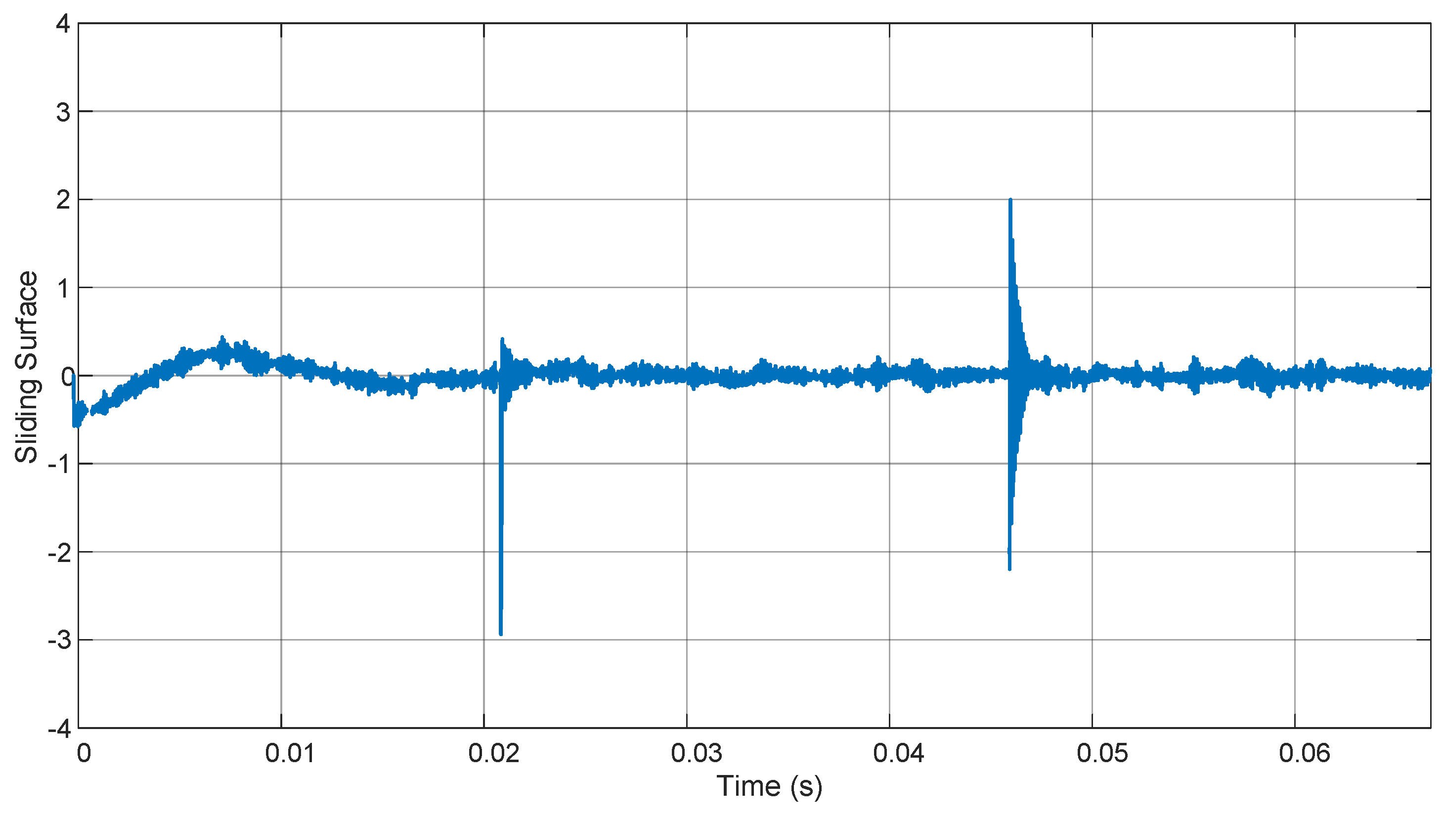
3. Results and Discussion

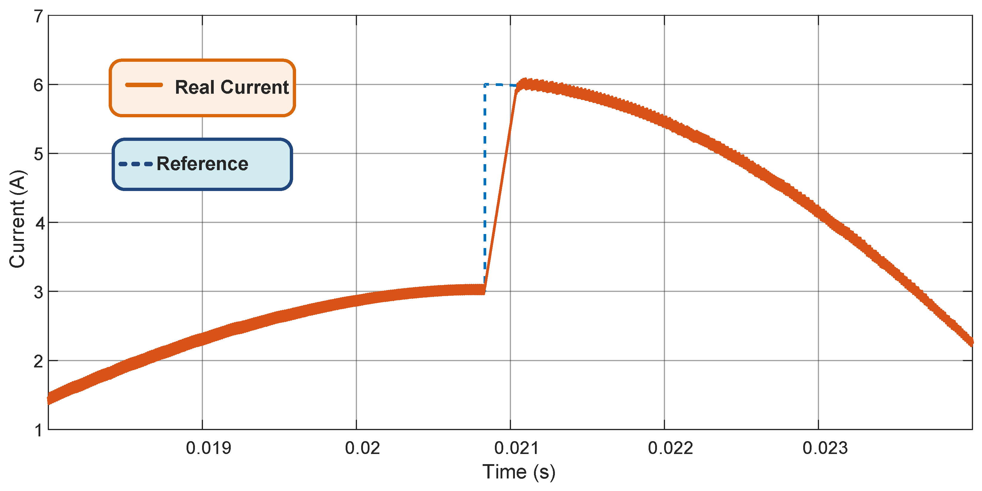
3.1. VSI Plus L Filter

The converter and the SMC control methodology were implemented in the MATLAB/Simulink® environment. The proposed control is depicted in the diagram in Figure 6. The power electronics converter obeyed the Figure 1 topology and Table 1 parameters. The PLL block received the grid voltage in p.u. and produced the ω t angle for popper synchronization. The PLL block was tuned using [15]. The sine and cosine functions resulted in values ranging from 1 to 1 .
The choice of ε and q values did not have an exact methodology. Through several simulation tests with different values, ε = 0.05 and q = 0.84 were chosen, seeking to achieve a response that had low THD (inferior to 5%), minimal reference tracking error, a small disturbance when applying a step change in the current reference, and a modulation index within its given limits, i.e., less than the unity. To improve the results, designers may use a metaheuristic algorithm, e.g., the Genetic Algorithm, to find the best coefficients for the controller through an initial random population that evolves on the basis of the evaluation of a fitness function that combines the error and the current THD [21].
The simulation scenario comprised the injection of active power into the grid, and the reference step changed from half power to full power and vice versa. As seen in Figure 7, the step variations were imposed on the reference current to analyze the tracking capacity of the proposed SMC method during the positive and negative peaks of the current waveform, i.e., the most critical points.
Figure 8 consists of an additional detail of Figure 7, highlighting the moment when the variation occurred at the positive peak of the reference.
There was an outstanding tracking capacity for both the steady-state time period and at the step variations in the reference current i 1 * . Figure 9 and Figure 10 can be observed to assess the behavior of the sliding surface and the control action of the proposed SMC method, respectively. One may observe that the control variable was between the values of 1 and 1 and the sliding surface was close to zero.
Another criterion that can be used to study the effectiveness of the control is the THD, which is present in the grid current. For this scenario, the harmonic current spectrum is displayed in Figure 11.
Considering the limits defined by international standards (such as IEEE 1547) [17], the value of 0.92% is much lower than the limit value of 5% established for these applications, indicating an outstanding result for the energy quality injected by the system.
Finally, Figure 12 presents the comparisons between the traditional SMC and the proposed one, showing the effectiveness of the current SMC with less chattering effect. Figure 12 presents the same power profile as Figure 8.

3.2. VSI Plus LCL Filter

The converter and the SMC control methodology were implemented in the MATLAB/Simulink® environment. The proposed control is depicted in the diagram in Figure 13. The power electronics converter obeyed the Figure 2 topology and Table 2 parameters. Despite the current ripples, i 1 and i 2 possess the same instantaneous average value, so L 1 d i 1 d t is approximated by L 1 d i 2 * d t in this diagram, and thus their maximum values are I p e a k _ r e f . To comply with the active damping through capacitor current feedback, K × I C a p was subtracted from the modulation index m .
The same current reference profile was adopted to test the SMC control for the LCL filter, and ε = 0.06 and q = 1.085 were chosen. The results are presented in Figure 14. The analysis of this result showed a constant tracking error due to the discontinuous portion δ u . With this approach, the THD level was approximately 5%. In order to reduce the effects of the signal function (sign) and improve the controller response, the sign function in δ u can be replaced with a hyperbolic tangent function (tanh). Different studies have shown the results of the latter function on various applications, as seen in [22,23], to reduce the discontinuities of the signal function. Using such an approach, the THD is reduced to 4%.
Even though the THD was improved, it was necessary to reduce the error in the reference tracking. This could be achieved by replacing the discontinuous portion δu with a proportional plus resonant (P + R) controller, which makes it possible to eliminate the steady-state error at a chosen frequency by adopting a design procedure for the P + R controller through the use of the Bode diagrams concept. For that, we used the MATLAB SISOtool toolbox to dynamically choose the P + R coefficients. The resulting controller is given by (27), where ω is the grid frequency. K p was chosen to have the same q gain, and K r was chosen as 250. This P + R controller produced a crossing-over frequency of approximately 1 3 f s .
G P R s = K p + K r s s 2 + ω 2 = 1.085 + 250 s s 2 + 377 2
Finally, the results of the SMC plus P + R controller are shown in Figure 15, Figure 16, Figure 17 and Figure 18. In Figure 15, one may see the real current and its reference; in Figure 16, one detail of the current step change is shown; in Figure 17, one may see the sliding surface; and finally, in Figure 18 one may see the control action. Through these results, one may verify null stead-state error.
Finally, for the scenario in Figure 15 with a full load, the harmonic current spectrum is displayed in Figure 19. The obtained THD was about 1.35%. Comparing the results obtained with Figure 11, the THD was a little bit higher but much less than the 5% allowed by the standards. This happened because the system with the LCL filter was more challenging to control than the unique L filter.
With the given results, both the sign and tanh function approaches showed similarities regarding the tracking error, with a small reduction in THD using the tanh function. Considering what was seen, the use of the SMC plus the P + R method seems to be the most appropriate, given that it had a lower THD and an important reduction in the tracking error between the currents (real and reference).

4. Conclusions

For the L filter, the results observed by the SMC method were extremely successful, considering that the THD was far below the limit of 5%; the tracking error between grid current i 1 and reference current i 1 * was close to zero; and the tracking capacity was good enough to follow the variation of the reference during the step with no overshoot, outperforming the conventional control.
The connection to the grid from an inverter with an LCL filter requires the use of an active damping technique to assist in attenuating the resonance frequency from the filter itself, considering lossless damping. In this regard, capacitor current feedback was adopted. Regarding the design of the SMC method, the signal function was not sufficient to maintain the energy quality criteria, in which, by using the tanh function, the response of the controller was improved. Despite the improvements, there was still a steady-state error, which could be reduced (or even eliminated) with the correct design of a P + R controller to substitute the sign function.
Therefore, with the P + R controller properly dimensioned, some improvements were seen in the tracking for the step variation and during the steady state, along with reduced tracking error between the grid current i 2 and the reference current i 2 * . It is necessary to highlight the flexibility of the SMC method in working with other types of controllers.
Finally, this paper reinforced that the obtainment of the equivalent control law in terms of the modulation index allows the system to reduce the chattering effect.

Author Contributions

Conceptualization, M.A.G.d.B. and E.H.B.D.; methodology, M.A.G.d.B.; software, E.H.B.D. and L.P.S.; validation, L.P.S. and R.C.G.; formal analysis, M.A.G.d.B. and R.C.G.; investigation, M.A.G.d.B. and E.H.B.D.; writing—original draft preparation, M.A.G.d.B. and S.A.O.d.S.; writing—review and editing, L.P.S. and S.A.O.d.S. All authors have read and agreed to the published version of the manuscript.

Funding

This research received no external funding.

Institutional Review Board Statement

Not applicable.

Informed Consent Statement

Not applicable.

Data Availability Statement

Not applicable.

Acknowledgments

The authors would like to thank the Federal University of Mato Grosso do Sul—UFMS and the Federal Technological University of Paraná—UTFPR.

Conflicts of Interest

The authors declare no conflict of interest.

Appendix A

Here, the steps for the obtainment of (18) through block diagram reduction are shown.
Figure A1. Obtainment of (18) through block diagram reduction (ah).
Eng 04 00018 g0a1

References

  1. Liserre, E.M.; Sauter, T.; Hung, J.Y. Future Energy Systems: Integrating Renewable Energy Sources into the Smart Power Grid Through Industrial Electronics. IEEE Trans. Ind. Electron. 2010, 4, 18–37. [Google Scholar] [CrossRef]
  2. REN21. Renewables 2019 Global Status Report. 2019. Available online: https://www.ren21.net/wp-content/uploads/2019/05/gsr_2019_full_report_en.pdf (accessed on 5 October 2021).
  3. IEA. Renewable Energy Market Update—May 2022. 2022. Available online: https://www.iea.org/reports/renewable-energy-market-update-may-2022 (accessed on 1 June 2022).
  4. Brito, M.A.G.; Sampaio, L.P.; Galotto, L., Jr.; Canesin, C.A. Evaluation of the Main MPPT Techniques for Photovoltaic Applications. IEEE Trans. Ind. Electron. 2013, 60, 1156–1167. [Google Scholar] [CrossRef]
  5. Hao, X.; Yang, X.; Liu, T.; Huang, L.; Chen, W. A Sliding-Mode Controller with Multi-Resonant Sliding Surface for Single-Phase Grid-Connected VSI with an LCL-Filter. IEEE Trans. Power Electron. 2013, 5, 2259–2268. [Google Scholar] [CrossRef]
  6. Hill, W.A.; Kapoor, S.C. Effect of Two-Level PWM Sources on Plant Power System Harmonics. In Proceedings of the Conference Record of 1998 IEEE Industry Applications Conference, St. Louis, MO, USA, 15 October 1998. [Google Scholar]
  7. Liserre, M.; Blaabjerg, F.; Hansen, S. Design and Control of an LCL-Filter-Based Three-Phase Active Rectifier. IEEE Trans. Ind. Appl. 2005, 41, 1281–1291. [Google Scholar] [CrossRef]
  8. Ruan, X.; Wang, X.; Pan, D.; Yang, D.; Li, W.; Bao, C. Control Techniques for LCL-Type Grid-Connected Inverters; Springer: Singapore, 2017. [Google Scholar]
  9. Santos, L.M.; Lucas, L.A.; Brito, M.A.G.; Garcia, R.C. Analysis of Digital Current Controllers for Single-Phase Grid-Connected Photovoltaic Inverters. In Proceedings of the Intercon, IEEE XXVI International Conference on Electronics, Electrical Engineering and Computing, Lima, Peru, 12–14 August 2019. [Google Scholar]
  10. Twining, E.; Holmes, D.G. Grid Current Regulation of a Three-Phase Voltage Source Inverter with an LCL Input Filter. IEEE Trans. Power Electron. 2003, 5, 888–895. [Google Scholar] [CrossRef] [Green Version]
  11. Vieira, R.P. Contribuições ao Acionamento e Controle Sensorless Aplicado ao Motor de Indução Bifásico Assimétrico. Ph.D. Thesis, Federal University of Santa Maria, Santa Maria, Brazil, 2012. [Google Scholar]
  12. De Oliveira, T.R. Controle por Modos Deslizantes de Sistemas Incertos com Direção de Controle Desconhecida. Ph.D. Thesis, Federal University of Rio de Janeiro, Rio de Janeiro, Brazil, 2006. [Google Scholar]
  13. Utkin, V.I. Variable Structure Systems with Sliding Modes. IEEE Trans. Autom. Control. 1977, 4, 212–222. [Google Scholar] [CrossRef]
  14. Gao, W.; Hung, J.C. Variable Structure Control of Nonlinear Systems: A New Approach. IEEE Trans. Ind. Electron. 1993, 2, 45–55. [Google Scholar]
  15. Svensson, J. Synchronization Methods for Grid-Connected Voltage Source Converters. IEE Proc. Gen. Transm. Distrib. 2001, 148, 229–235. [Google Scholar] [CrossRef] [Green Version]
  16. Erickson, R.W.; Maksimovic, D. Fundamentals of Power Electronics, 2nd ed.; Kluwer Academic Publisher: Amsterdam, The Netherlands, 2000. [Google Scholar]
  17. Chang, L.; Song, P.; Diduch, C. Development of Standards for Interconnecting Distributed Generators with Electric Power Systems. In Proceedings of the IEEE Annual Power Electronics Specialists Conference, Recife, Brazil, 12–16 June 2005. [Google Scholar]
  18. Jia, Y.; Zhao, J.; Fu, X. Direct Grid Current Control of LCL-Filtered Grid-Connected Inverter Mitigating Grid Voltage Disturbance. IEEE Trans. Power Electron. 2013, 29, 1532–1541. [Google Scholar]
  19. Ogata, K. Modern Control Engineering; Prentice Hall: Hoboken, NJ, USA, 2020. [Google Scholar]
  20. De Vegte, J. Feedback Control Systems, 3rd revised ed.; Prentice Hall: Hoboken, NJ, USA, 1993. [Google Scholar]
  21. Lucas, L.A.; Brito, M.A.G.; Garcia, R.C. A photovoltaic multi-functional converter with multi-resonant controller coefficients improved by a genetic algorithm. In Proceedings of the Intercon, IEEE XXVI International Conference on Electronics, Electrical Engineering and Computing, Lima, Peru, 12–14 August 2019. [Google Scholar]
  22. Song, F.; Smith, S.M. Design of Sliding Mode Fuzzy Controllers for an Autonomous Underwater Vehicle without System Model. In Proceedings of the OCEANS 2000 MTS/IEEE Conference and Exhibition, Providence, RI, USA, 11–14 September 2000; Volume 9, pp. 835–840. [Google Scholar]
  23. Glower, J.S.; Munighan, J. Designing Fuzzy Controllers from a Variable Structures Standpoint. IEEE Trans. Fuzzy Syst. 1997, 2, 138–144. [Google Scholar] [CrossRef]
Figure 1. Single-phase VSI with the L filter.
Eng 04 00018 g001
Figure 2. Single-phase VSI with the LCL filter.
Eng 04 00018 g002
Figure 3. Frequency analysis of the designed LCL filter.
Eng 04 00018 g003
Figure 4. Block diagram of the active damping. V i n v = m V D C , i L 1 = i 1 , i L 2 = i 2 , and v g = v g r i d .
Eng 04 00018 g004
Figure 5. Frequency analysis of the damped LCL filter.
Eng 04 00018 g005
Figure 6. SMC control diagram strategy for the single-phase VSI with the L filter.
Eng 04 00018 g006
Figure 7. Comparison between currents i 1 * and i 1 .
Eng 04 00018 g007
Figure 8. Comparison between currents i 1 * and i 1 —in detail.
Eng 04 00018 g008
Figure 9. Tracking error between currents i 1 * and i 1 .
Eng 04 00018 g009
Figure 10. Control action u s m c over time to produce the switching states.
Eng 04 00018 g010
Figure 11. Grid current harmonic spectrum with the L filter.
Eng 04 00018 g011
Figure 12. Comparison of the traditional and proposed SMCs.
Eng 04 00018 g012
Figure 13. Proposed SMC control diagram strategy. I C a p = I C .
Eng 04 00018 g013
Figure 14. Comparison between currents i 2 and i 2 * using the signal function.
Eng 04 00018 g014
Figure 15. Comparison between currents i 2 and i 2 * with SMC plus P + R.
Eng 04 00018 g015
Figure 16. Step response tracking with SMC plus P + R.
Eng 04 00018 g016
Figure 17. Tracking error between currents i 2 and i 2 * with SMC plus P + R.
Eng 04 00018 g017
Figure 18. Control action u s m c for reference i 2 * with SMC plus P + R.
Eng 04 00018 g018
Figure 19. Grid current harmonic spectrum with the LCL filter.
Eng 04 00018 g019
Table 1. Parameters for designing the L filter.
ParametersValue
Output power500 W
Input voltage250 V
Grid RMS voltage127 V
Grid fundamental Frequency60 Hz
Switching frequency40 kHz
Grid current ripple4.5%
Table 2. LCL filter parameters.
ComponentValue
Inductance   L 1 1.65 mH
Inductance   L 2 25.7 µH
Capacitance   C f 6.5 µF
Disclaimer/Publisher’s Note: The statements, opinions and data contained in all publications are solely those of the individual author(s) and contributor(s) and not of MDPI and/or the editor(s). MDPI and/or the editor(s) disclaim responsibility for any injury to people or property resulting from any ideas, methods, instructions or products referred to in the content.

