Dispersive Optical Solitons for Stochastic Fokas-Lenells Equation With Multiplicative White Noise

Abstract

For the first time, we study the Fokas–Lenells equation in polarization preserving fibers with multiplicative white noise in Itô sense. Four integration algorithms are applied, namely, the method of modified simple equation (MMSE), the method of sine-cosine (MSC), the method of Jacobi elliptic equation (MJEE) and ansatze involving hyperbolic functions. Jacobi-elliptic function solutions, bright, dark, singular, combo dark-bright and combo bright-dark solitons are presented.

1. Introduction

Nonlinear differential equations (NLDEs) play a very important role in scientific fields and engineering such as optical fibers, the heat flow, plasma physics, solid-state physics, chemical kinematics, the proliferation of shallow water waves, fluid mechanics, quantum mechanics, wave proliferation phenomena, etc. One of the fundamental physical problems for these models is to obtain their traveling wave solutions. As a consequence, the search for mathematical methods to create exact solutions of NLDEs is an important and essential activity in nonlinear sciences. In recent years, many articles have studied optical solitons’ form in telecommunications industry. These soliton molecules form the information transporter across intercontinental distances around the world. Lastly, the nonlinear Schrödinger’s equation (NLSE) has been discussed with the help of many models [1,2,3,4,5,6,7,8,9,10,11,12,13,14,15,16,17,18,19,20,21,22,23,24,25,26,27,28,29,30,31,32,33,34,35,36,37,38]. The aspect of stochasticity is one of the features that is less touched upon and there are hardly any papers that have debated this point [3,4,5,6,7,8,9]. The Fokas–Lenells equation (FLE) appears as a model which appoints nonlinear pulse propagation in optical fibers. The FLE is a completely integrable equation which has arisen as an integrable generalization of the NLSE using bi-Hamiltonian methods [10]. On the other hand, the FLE models have the propagation of nonlinear light pulses in monomode optical fibers when certain higher-order nonlinear effects are considered in optics field [11]. The complete integrability of the FLE has been presented by using the inverse scattering transform (IST) method [12]. In the main, a Lax pair and a few conservation laws connected to it have been obtained using the bi-Hamiltonian structure and the multi-soliton solutions have been derived by using the dressing method [13]. One more main characteristic of the FLE is that it is the first negative flow of the integrable hierarchy of the derivative NLSE [14].

In the present article, we will study the FLE with multiplicative white noise in the Itô sense. Our results are presented after a comprehensive analysis obtained in this article.

2. Governing Model

The dimensionless structure of the stochastic perturbed FLE in polarization preserving fiber with multiplicative white noise in the Itô sense is written, for the first time, as:

$$i{q}_t+a_1{q}_{xx}+a_2{q}_{xt}+{\left|q\right|}^2(bq+ic{q}_x)+\sigma (q-i{a}_2{q}_x)\frac{dW\left(t\right)}{dt}=i\left[\alpha q_x+\lambda {\left({\left|q\right|}^{2}q\right)}_x+\mu {\left({\left|q\right|}^2\right)}_{x}q\right],$$

(1)

where $q(x,t)$ is a complex-valued function that represents the wave profile, while $a_1, a_2, b, c,$$\sigma , \alpha , \lambda , \mu$ are real-valued constants and $i=\sqrt{-1}$. The first term in Equation (1) is the linear temporal evolution, $a_1$ is the coefficient of chromatic dispersion (CD), $a_2$ is the coefficient of spatio-temporal dispersion (STD), b is the coefficient of self-phase modulation (SPM), c is the coefficient of nonlinear dispersion term, $\sigma$ is the coefficient of the strength of noise, the Wiener process is denoted by $W\left(t\right)$, while $dW\left(t\right)/dt$ represents the white noise. Also, the term $dW\left(t\right)/dt$ is the time derivative of the standard Wiener process $W\left(t\right)$ which is called a Brownian motion and has the following properties [7]: (i) $W\left(t\right),t\ge 0,$ is a continuous function of t, (ii) For $s<t,W\left(t\right)-W\left(s\right)$ is independent of increments. (iii) $W\left(t\right)-W\left(s\right)$ has a normal distribution with mean zero and variance $(t-s)$.

Next, $\alpha$ is the coefficient of inter-modulation dispersion (IMD), $\lambda$ is the coefficient of self-steepening (SS) term, and finally $\mu$ is the coefficient of higher-order nonlinear dispersion term. If $\sigma =0$, Equation (1) reduces to the familiar FLE which is studied in [1,2,37]. The authors [37] studied Equation (1) with variable coefficients and $\sigma =0$. The motivation of adding the stochastic term $\sigma (q-i{a}_2{q}_x)\frac{dW\left(t\right)}{dt}$ to Equation (1) is to formulate the stochastic FLE with noise or fluctuations depending on the time, which has been recognized in many areas via physics, engineering, chemistry and so on. This stochastic term has been constructed with the help of the two terms $i{q}_t$ and $a_2{q}_{xt}$. Therefore, in general, the stochastic model means that the model of differential equations should contain the white noise term ($\sigma \ne 0$). The physical importance of the stochastic FL Equation (1) is to find its traveling wave stochastic solutions which appoint the nonlinear pulse propagations in optical fibers.

The aim of this article is to use the method of MMSE in Section 3, the method of MSC in Section 4, the method of MJEE in Section 5 and the ansatze involving hyperbolic functions in Section 6 to find the bright, dark, singular soliton solutions, as well as the Jacobi elliptic function solutions of Equation (1). Some numerical simulations are obtained in Section 7. Finally, conclusions are illustrated in Section 8.

3. On Solving Equation (1) by MMSE

In order to solve the stochastic Equation (1), we use a wave transformation involving the noise coefficient $\sigma$ and the Wiener process $W\left(t\right)$ in the form:

$$q(x,t)=\varphi \left(\xi \right)expi\left[-\kappa x+wt+\sigma W\left(t\right)-{\sigma }^{2}t\right],$$

(2)

where the transformation $\xi =x-vt$ is used. Here, $\kappa ,w,v,$ are real constants, such that $\kappa$ represents the wave number, w represents the frequency and v represents the soliton velocity. The function $\varphi \left(\xi \right)$ is real function which represents the amplitude part. When we put Equation (2) into Equation (1), we obtain the ordinary differential equation (ODE):

$$\left[a_1-a_{2}v\right]{\varphi }^{″}+Y\varphi +\left[b+\kappa \left(c-\lambda \right)\right]{\varphi }^3=0,$$

(3)

and the soliton velocity,

$$v=\frac{Y}{(a_2\kappa -1)},a_2\kappa \ne 1$$

(4)

as well as the constraint condition,

$$c-3\lambda -2\mu =0,$$

(5)

where $Y=\left[(w-{\sigma }^2)(a_2\kappa -1)-a_1{\kappa }^2-\alpha \kappa \right]$ and ${}^{″}=\frac{d^2}{d{\xi }^2}$. We have the balance number $N=1$ by balancing ${\varphi }^{″}$ with the ${\varphi }^3$ in Equation (3). According to the method of MSE [15,16,17,18,19,20], the solution of Equation (3) is written as:

$$\varphi \left(\xi \right)=A_0+A_1\left[\frac{{\psi }^{\prime }\left(\xi \right)}{\psi \left(\xi \right)}\right],$$

(6)

where $\psi \left(\xi \right)$ is a new function of $\xi$, and $A_0,A_1$ are constants to be determined later, provided $A_1\ne 0,$$\psi \left(\xi \right)\ne 0$ and ${\psi }^{\prime }\left(\xi \right)\ne 0.$

Inserting Equation (6) into Equation (3), and collecting all the coefficients of ${\psi }^{-i}\left(\xi \right)$$\left(i=0,1,2,3\right)$, we obtain the equations:

$${\psi }^0:A_{0}Y+A_0^3\left[b+\kappa \left(c-\lambda \right)\right]=0,$$

(7)

$${\psi }^{-1}:A_1{\psi }^{‴}\left[a_1-a_{2}v\right]+A_1\psi Y+3A_0^2{A}_1{\psi }^{\prime }\left[b+\kappa \left(c-\lambda \right)\right]=0,$$

(8)

$${\psi }^{-2}:-3A_1{\psi }^{\prime }{\psi }^{″}\left[a_1-a_{2}v\right]+3A_0{A}_1^2{\psi }^{\prime 2}\left[b+\kappa \left(c-\lambda \right)\right]=0,$$

(9)

$${\psi }^{-3}:2A_1{\psi }^{\prime 3}\left[a_1-a_{2}v\right]+A_1^3{\psi }^{\prime 3}\left[b+\kappa \left(c-\lambda \right)\right]=0.$$

(10)

By solving Equations (7) and (10), we obtain:

$$A_0=0,A_0=\pm \sqrt{-\frac{Y}{\left[b+\kappa \left(c-\lambda \right)\right]}},A_1=\pm \sqrt{-\frac{2\left[a_1-a_{2}v\right]}{\left[b+\kappa \left(c-\lambda \right)\right]},}$$

(11)

provided $\left[b+\kappa \left(c-\lambda \right)\right]Y<0$ and $\left[b+\kappa \left(c-\lambda \right)\right]\left[a_1-a_{2}v\right]<0.$

By solving Equations (8) and (9), we conclude that $A_0=0$ is rejected. Therefore, $A_0\ne 0$. Now, Equation (9) reduces to the ODE:

$$\left[a_1-a_{2}v\right]{\psi }^{″}-A_0{A}_1\left[b+\kappa \left(c-\lambda \right)\right]{\psi }^{\prime }=0,$$

(12)

which has the solution

$${\psi }^{\prime }\left(\xi \right)={\xi }_{0}exp\left[\frac{A_0{A}_1\left[b+\kappa \left(c-\lambda \right)\right]}{\left[a_1-a_{2}v\right]}\xi \right],$$

(13)

where ${\xi }_0$$\ne 0$ is a constant. From Equation (11) and Equation (13), we can show that Equation (8) is valid. Hence, we have the results:

$$\psi \left(\xi \right)=\frac{{\xi }_0\left[a_1-a_{2}v\right]}{A_0{A}_1\left[b+\kappa \left(c-\lambda \right)\right]}exp\left[\frac{A_0{A}_1\left[b+\kappa \left(c-\lambda \right)\right]}{\left[a_1-a_{2}v\right]}\xi \right]+{\xi }_1,$$

(14)

where ${\xi }_1$ is a nonzero constant of integration. Now, the exact solution of Equation (1) has the form:

$$q(x,t)=\left\{A_0+A_1\frac{{\xi }_{0}exp\left[\frac{A_0{A}_1\left[b+\kappa \left(c-\lambda \right)\right]}{\left[a_1-a_{2}v\right]}\left(x-vt\right)\right]}{{\xi }_1+\frac{{\xi }_0\left[a_1-a_{2}v\right]}{A_0{A}_1\left[b+\kappa \left(c-\lambda \right)\right]}exp\left[\frac{A_0{A}_1\left[b+\kappa \left(c-\lambda \right)\right]}{\left[a_1-a_{2}v\right]}\left(x-vt\right)\right]}\right\}expi\left[-\kappa x+wt+\sigma W\left(t\right)-{\sigma }^{2}t\right].$$

(15)

In particular, if we set,

$${\xi }_1=\frac{{\xi }_0\left[a_1-a_{2}v\right]}{A_0{A}_1\left[b+\kappa \left(c-\lambda \right)\right]},$$

(16)

we have the dark soliton solution:

$$q(x,t)=\pm \sqrt{-\frac{Y}{\left[b+\kappa \left(c-\lambda \right)\right]}}tanh\left[\sqrt{\frac{Y}{2\left[a_1-a_{2}v\right]}}\left(x-vt\right)\right]expi\left[-\kappa x+wt+\sigma W\left(t\right)-{\sigma }^{2}t\right],$$

(17)

while, if we set,

$${\xi }_1=-\frac{{\xi }_0\left[a_1-a_{2}v\right]}{A_0{A}_1\left[b+\kappa \left(c-\lambda \right)\right]},$$

(18)

we have the singular soliton solution:

$$q(x,t)=\pm \sqrt{-\frac{Y}{\left[b+\kappa \left(c-\lambda \right)\right]}}coth\left[\sqrt{\frac{Y}{2\left[a_1-a_{2}v\right]}}\left(x-vt\right)\right]expi\left[-\kappa x+wt+\sigma W\left(t\right)-{\sigma }^{2}t\right],$$

(19)

provided,

$$\left[b+\kappa \left(c-\lambda \right)\right]Y<0,\left[a_1-a_{2}v\right]Y>0.$$

(20)

On comparing our above results (17) and (19) with the results (19) and (20) obtained in [37], we deduce that they are equivalent when $\sigma =0.$

4. On Solving Equation (1) by MSC

To apply this method according to [21,22,23,24,25], assume that Equation (3) has the sine-solution form:

$$\varphi \left(\xi \right)=\left\{\begin{array}{c}{\lambda }_1{sin}^{{\beta }_1}\left({\mu }_1\xi \right),\mathrm{if}\left|\xi \right|<\frac{\pi }{{\mu }_1},\\ 0,\mathrm{otherwise}.\end{array}\right.$$

(21)

Substituting Equation (21) into Equation (3), we obtain:

$$\begin{array}{c}\left[a_1-a_{2}v\right]\left[{\lambda }_1{\mu }_1^2{\beta }_1({\beta }_1-1){sin}^{{\beta }_1-2}\left({\mu }_1\xi \right)-{\lambda }_1{\mu }_1^2{\beta }_1^2{sin}^{{\beta }_1}\left({\mu }_1\xi \right)\right]\\ \\ +Y{\lambda }_1{sin}^{{\beta }_1}\left({\mu }_1\xi \right)+\left[b+\kappa \left(c-\lambda \right)\right]{\lambda }_1^3{sin}^{3{\beta }_1}\left({\mu }_1\xi \right)=0.\end{array}$$

(22)

From (22), we deduce that ${\beta }_1-2=3{\beta }_1$ which leads ${\beta }_1=-1$. Consequently, we have the results:

$${\mu }_1^2=\frac{Y}{\left[a_1-a_{2}v\right]},{\lambda }_1^2=-\frac{2Y}{\left[b+\kappa \left(c-\lambda \right)\right]}.$$

(23)

Now, the periodic solution of Equation (1) is:

$$q(x,t)=\pm \sqrt{-\frac{2Y}{\left[b+\kappa \left(c-\lambda \right)\right]}}csc\left[\sqrt{\frac{Y}{\left[a_1-a_{2}v\right]}}\left(x-vt\right)\right]expi\left[-\kappa x+wt+\sigma W\left(t\right)-{\sigma }^{2}t\right],$$

(24)

provided $\left[b+\kappa \left(c-\lambda \right)\right]Y<0$, $\left[a_1-a_{2}v\right]Y>0.$

Since $csc\left(ix\right)=-i\mathrm{c}\mathrm{s}\mathrm{c}\mathrm{h}x,$ then the singular soliton solution of Equation (1) is written as:

$$q(x,t)=\pm \sqrt{\frac{2Y}{\left[b+\kappa \left(c-\lambda \right)\right]}}\mathrm{c}\mathrm{s}\mathrm{c}\mathrm{h}\left[\sqrt{-\frac{Y}{\left[a_1-a_{2}v\right]}}\left(x-vt\right)\right]expi\left[-\kappa x+wt+\sigma W\left(t\right)-{\sigma }^{2}t\right],$$

(25)

provided $Y\left[b+\kappa \left(c-\lambda \right)\right]>0$, $\left[a_1-a_{2}v\right]Y<0.$

In parallel, if we allow that Equation (3) has the cosine-solution:

$$\varphi \left(\xi \right)=\left\{\begin{array}{c}{\lambda }_1{cos}^{{\beta }_1}\left({\mu }_1\xi \right),\mathrm{if}\left|\xi \right|<\frac{\pi }{2{\mu }_1},\\ \\ 0,\mathrm{otherwise}.\end{array}\right.$$

(26)

Putting Equation (26) into Equation (3), we obtain

$$\begin{array}{c}\left[a_1-a_{2}v\right]\left[-{\mu }_1^2{\beta }_1^2{\lambda }_1{cos}^{{\beta }_1}\left({\mu }_1\xi \right)+{\lambda }_1{\mu }_1^2{\beta }_1({\beta }_1-1){cos}^{{\beta }_1-2}\left({\mu }_1\xi \right)\right]\\ \\ +Y{\lambda }_1{cos}^{{\beta }_1}\left({\mu }_1\xi \right)+\left[b+\kappa \left(c-\lambda \right)\right]{\lambda }_1^3{cos}^{3{\beta }_1}\left({\mu }_1\xi \right)=0.\end{array}$$

(27)

From Equation (27), we deduce that ${\beta }_1-2=3{\beta }_1$, which leads ${\beta }_1=-1$. Therefore, we have the solutions:

$$q(x,t)=\pm \sqrt{-\frac{2Y}{\left[b+\kappa \left(c-\lambda \right)\right]}}sec\left[\sqrt{\frac{Y}{\left[a_1-a_{2}v\right]}}\left(x-vt\right)\right]expi\left[-\kappa x+wt+\sigma W\left(t\right)-{\sigma }^{2}t\right],$$

(28)

with conditions $\left[b+\kappa \left(c-\lambda \right)\right]Y<0$, $\left[a_1-a_{2}v\right]Y>0.$

Since, $sec\left(ix\right)=\mathrm{s}\mathrm{e}\mathrm{c}\mathrm{h}x,$ we have the bright soliton solution:

$$q(x,t)=\pm \sqrt{-\frac{2Y}{\left[b+\kappa \left(c-\lambda \right)\right]}}\mathrm{s}\mathrm{e}\mathrm{c}\mathrm{h}\left[\sqrt{-\frac{Y}{\left[a_1-a_{2}v\right]}}(x-vt)\right]expi\left[-\kappa x+wt+\sigma W\left(t\right)-{\sigma }^{2}t\right],$$

(29)

provided $\left[b+\kappa \left(c-\lambda \right)\right]Y<0$, $\left[a_1-a_{2}v\right]Y<0.$

5. On Solving Equation (1) by MJEE

If we multiply Equation (3) by ${\varphi }^{\prime }\left(\xi \right)$ and integrate, we have the JEE as:

$${\varphi }^{\prime 2}\left(\xi \right)=l_0+l_2{\varphi }^2\left(\xi \right)+l_4{\varphi }^4\left(\xi \right),$$

(30)

where,

$$l_0=\frac{2c_1}{\left[a_1-a_{2}v\right]},l_2=-\frac{Y}{\left[a_1-a_{2}v\right]},l_4=-\frac{\left[b+\kappa \left(c-\lambda \right)\right]}{2\left[a_1-a_{2}v\right]},$$

(31)

and $c_1$ is the integration constant, $\left[a_1-a_{2}v\right]\ne 0.$ It is noted [26,27,28,29,30] that Equation (30) has the Jacobi-elliptic solutions in the forms:

(1) If $l_0=1,l_2=-\left(1+m^2\right),l_4=m^2$, $0<m<1,$ then,

$$\varphi \left(\xi \right)=sn\left(\xi \right)\mathrm{or}\varphi \left(\xi \right)=cd\left(\xi \right).$$

(32)

Then, Equation (1) has the JEE solution:

$$\begin{array}{c}q(x,t)=sn(x-vt)expi\left[-\kappa x+wt+\sigma W\left(t\right)-{\sigma }^{2}t\right],\hfill \\ \mathrm{or}\hfill \\ q(x,t)=cd(x-vt)expi\left[-\kappa x+wt+\sigma W\left(t\right)-{\sigma }^{2}t\right],\hfill \end{array}$$

(33)

where,

$$\begin{array}{c}{c}_1=\frac{1}{2}\left(a_1-a_{2}v\right),\hfill \\ Y=(1+m^2)(a_1-a_{2}v),\hfill \\ b+\kappa \left(c-\lambda \right)=-2m^2(a_1-a_{2}v),\hfill \end{array}$$

(34)

and consequently, we obtain

$$Y=-\frac{(1+m^2)}{2m^2}\left[b+\kappa \left(c-\lambda \right)\right].$$

Particularly, if $m\to 1,$ we get,

$$q(x,t)=tanh(x-vt)expi\left[-\kappa x+wt+\sigma W\left(t\right)-{\sigma }^{2}t\right].$$

(35)

Note that the solution Equation (35) is equivalent to the solution Equation (17) under the conditions of Equation (34).

(2) If $l_0=m^2,l_2=-\left(1+m^2\right),l_4=1$, $0<m<1,$ then,

$$\varphi \left(\xi \right)=ns\left(\xi \right)\mathrm{or}\varphi \left(\xi \right)=dc\left(\xi \right).$$

(36)

Then, we obtain the JEE solution for Equation (1),

$$\begin{array}{c}q(x,t)=ns(x-vt)expi\left[-\kappa x+wt+\sigma W\left(t\right)-{\sigma }^{2}t\right],\hfill \\ \mathrm{or}\hfill \\ q(x,t)=dc(x-vt)expi\left[-\kappa x+wt+\sigma W\left(t\right)-{\sigma }^{2}t\right],\hfill \end{array}$$

(37)

where,

$$\begin{array}{c}{c}_1=\frac{1}{2}{m}^2\left(a_1-a_{2}v\right),\hfill \\ Y=(1+m^2)(a_1-a_{2}v),\hfill \\ b+\kappa \left(c-\lambda \right)=-2(a_1-a_{2}v),\hfill \end{array}$$

(38)

and consequently, we have,

$$Y=-\frac{(1+m^2)}{2}\left[b+\kappa \left(c-\lambda \right)\right].$$

Particularly, if $m\to 1,$ we obtain,

$$q(x,t)=coth(x-vt)expi\left[-\kappa x+wt+\sigma W\left(t\right)-{\sigma }^{2}t\right].$$

(39)

Note that the solution in Equation (39) is equivalent to the solution in Equation (19) under the conditions in Equation (38).

(3) If $l_0=1-m^2,l_2=2m^2-1,l_4=-m^2$, $0<m<1,$ then,

$$\varphi \left(\xi \right)=\mathrm{cn}\left(\xi \right).$$

(40)

Now, we have the JEE solution for Equation (1),

$$q(x,t)=\mathrm{cn}\left(x-vt\right)expi\left[-\kappa x+wt+\sigma W\left(t\right)-{\sigma }^{2}t\right],$$

(41)

where,

$$\begin{array}{c}{c}_1=\frac{1}{2}(1-m^2)\left(a_1-a_{2}v\right),\hfill \\ Y=-(2m^2-1)(a_1-a_{2}v),\hfill \\ b+\kappa \left(c-\lambda \right)=2m^2(a_1-a_{2}v),\hfill \end{array}$$

(42)

and consequently, we have,

$$Y=-\frac{(2m^2-1)}{2m^2}\left[b+\kappa \left(c-\lambda \right)\right].$$

Particularly, if $m\to 1,$ we obtain,

$$q(x,t)=\mathrm{s}\mathrm{e}\mathrm{c}\mathrm{h}\left(x-vt\right)expi\left[-\kappa x+wt+\sigma W\left(t\right)-{\sigma }^{2}t\right]$$

(43)

Note that the solution of Equation (43) is equivalent to the solution of Equation (29) under the conditions of Equation (42).

(4) If $l_0=-m^2\left(1-m^2\right),l_2=2m^2-1,l_4=1$, $0<m<1,$ then,

$$\varphi \left(\xi \right)=ds\left(\xi \right).$$

(44)

Consequently, we have the JEE solution for Equation (1),

$$q(x,t)=ds\left(x-vt\right)expi\left[-\kappa x+wt+\sigma W\left(t\right)-{\sigma }^{2}t\right],$$

(45)

where,

$$\begin{array}{c}{c}_1=-\frac{m^2}{2}(1-m^2)\left(a_1-a_{2}v\right),\hfill \\ Y=-(2m^2-1)(a_1-a_{2}v),\hfill \\ b+\kappa \left(c-\lambda \right)=-2(a_1-a_{2}v),\hfill \end{array}$$

(46)

and we have,

$$Y=\frac{1}{2}(2m^2-1)\left[b+\kappa \left(c-\lambda \right)\right].$$

Particularly, if $m\to 1,$ we obtain

$$q(x,t)=\mathrm{c}\mathrm{s}\mathrm{c}\mathrm{h}\left(x-vt\right)expi\left[-\kappa x+wt+\sigma W\left(t\right)-{\sigma }^{2}t\right],$$

(47)

Note that the solution of Equation (47) is equivalent to the solution of Equation (25) under the conditions of Equation (46).

(5) If $l_0=\frac{1}{4},l_2=\frac{1}{2}(1-2m^2),l_4=\frac{1}{4}$, $0<m<1,$ then,

$$\varphi \left(\xi \right)=\frac{\mathrm{s}\mathrm{n}\left(\xi \right)}{1\pm \mathrm{c}\mathrm{n}\left(\xi \right)}.$$

(48)

Now, we have the JEE solution for the Equation (1),

$$q(x,t)=\frac{\mathrm{s}\mathrm{n}\left(x-vt\right)}{1\pm \mathrm{c}\mathrm{n}\left(x-vt\right)}expi\left[-\kappa x+wt+\sigma W\left(t\right)-{\sigma }^{2}t\right],$$

(49)

where,

$$\begin{array}{c}{c}_1=\frac{1}{8}\left(a_1-a_{2}v\right),\hfill \\ Y=-\frac{1}{2}(1-2m^2)(a_1-a_{2}v),\hfill \\ b+\kappa \left(c-\lambda \right)=-\frac{1}{2}(a_1-a_{2}v),\hfill \end{array}$$

(50)

and consequently, we have,

$$Y=(1-2m^2)\left[b+\kappa \left(c-\lambda \right)\right].$$

Particularly, if $m\to 1,$ we obtain the combo dark-bright soliton solutions:

$$q(x,t)=\frac{tanh\left(x-vt\right)}{1\pm \mathrm{s}\mathrm{e}\mathrm{c}\mathrm{h}\left(x-vt\right)}expi\left[-\kappa x+wt+\sigma W\left(t\right)-{\sigma }^{2}t\right].$$

(51)

(6) If $l_0=\frac{1-m^2}{4},l_2=\frac{1+m^2}{2},l_4=\frac{1-m^2}{4}$, $0<m<1,$ then,

$$\varphi \left(\xi \right)=\frac{\mathrm{c}\mathrm{n}\left(\xi \right)}{1\pm \mathrm{s}\mathrm{n}\left(\xi \right)}.$$

(52)

Then, we have the JEE solution for Equation (1),

$$q(x,t)=\frac{\mathrm{c}\mathrm{n}\left(x-vt\right)}{1\pm \mathrm{s}\mathrm{n}\left(x-vt\right)}expi\left[-\kappa x+wt+\sigma W\left(t\right)-{\sigma }^{2}t\right],$$

(53)

where

$$\begin{array}{c}{c}_1=\frac{1}{8}(1-m^2)\left(a_1-a_{2}v\right),\hfill \\ Y=-\frac{1}{2}(1+m^2)(a_1-a_{2}v),\hfill \\ b+\kappa \left(c-\lambda \right)=-\frac{1}{2}(1-m^2)(a_1-a_{2}v).\hfill \end{array}$$

(54)

Particularly, if $m\to 1,$ we obtain the combo bright-dark soliton solutions:

$$q(x,t)=\frac{\mathrm{s}\mathrm{e}\mathrm{c}\mathrm{h}\left(x-vt\right)}{1\pm tanh\left(x-vt\right)}expi\left[-\kappa x+wt+\sigma W\left(t\right)-{\sigma }^{2}t\right].$$

(55)

Finally, there are many other Jacobi elliptic solutions which are omitted here for simplicity.

6. Ansatze Involving Hyperbolic Functions

To this aim, we first write Equation (3) in the simple form,

$$A{\varphi }^{″}+Y\varphi +C{\varphi }^3=0,$$

(56)

where,

$$\begin{array}{c}A=a_1-a_{2}v,\hfill \\ C=b+\kappa \left(c-\lambda \right).\hfill \end{array}$$

(57)

Along these lines, the main steps of the proposed ansatze have been presented according to the ansatze involving the hyperbolic functions method [31].

6.1. Combo Bright-Dark Solitons

We assume the ansatz,

$$\varphi \left(\xi \right)=\frac{{\alpha }_1\mathrm{s}\mathrm{e}\mathrm{c}\mathrm{h}\left({\mu }_1\xi \right)}{1+{\lambda }_{1}tanh\left({\mu }_1\xi \right)}.$$

(58)

where ${\alpha }_1,{\lambda }_1,{\mu }_1$ are parameters to be determined. Now, we obtain

$${\varphi }^{″}\left(\xi \right)=\frac{{\alpha }_1{\mu }_1^2(2{\lambda }_1^2-1)\mathrm{s}\mathrm{e}\mathrm{c}\mathrm{h}\left({\mu }_1\xi \right)+2{\alpha }_1{\lambda }_1{\mu }_1^2\mathrm{s}\mathrm{e}\mathrm{c}\mathrm{h}\left({\mu }_1\xi \right)tanh\left({\mu }_1\xi \right)+{\alpha }_1{\mu }_1^2(2-{\lambda }_1^2)\mathrm{s}\mathrm{e}\mathrm{c}\mathrm{h}\left({\mu }_1\xi \right){tanh}^2\left({\mu }_1\xi \right)}{{\left(1+{\lambda }_{1}tanh\left({\mu }_1\xi \right)\right)}^3}.$$

(59)

Substituting Equations (58) and (59) into Equation (56), combining all the coefficients of ${\mathrm{s}\mathrm{e}\mathrm{c}\mathrm{h}}^p\left(\xi \right){tanh}^q\left(\xi \right)$$\left(p=1,q=0,1,2\right)$, we obtain the set of equations:

$$\begin{array}{c}A{\alpha }_1{\mu }_1^2(2{\lambda }_1^2-1)+Y{\alpha }_1+C{\alpha }_1^3=0,\\ 2A{\alpha }_1{\lambda }_1{\mu }_1^2+2Y{\alpha }_1{\lambda }_1=0,\\ A{\alpha }_1{\mu }_1^2(2-{\lambda }_1^2)+Y{\alpha }_1{\lambda }_1^2-C{\alpha }_1^3=0.\end{array}$$

(60)

By resolving the Equation (60), we have the results:

$${\mu }_1^2=\frac{-Y}{A},AY<0,{\lambda }_1^2=\frac{2Y+C{\alpha }_1^2}{2Y}>0,{\alpha }_1\ne 0.$$

Now, we obtain

$$q(x,t)=\left\{\frac{{\alpha }_1\mathrm{s}\mathrm{e}\mathrm{c}\mathrm{h}\left[\sqrt{\frac{-Y}{A}}(x-vt)\right]}{1\pm \sqrt{\frac{2Y+C{\alpha }_1^2}{2Y}}tanh\left[\sqrt{\frac{-Y}{A}}(x-vt)\right]}\right\}expi\left[-\kappa x+wt+\sigma W\left(t\right)-{\sigma }^{2}t\right].$$

(61)

which represent the combo-bright-dark soliton solutions and are equivalent to the solutions Equation (55) of Section 5, if $A=-Y$, $C=0$ and ${\alpha }_1=1.$

6.2. Combo Dark-Bright Solitons

We assume the ansatz

$$\varphi \left(\xi \right)=\frac{{\alpha }_{1}tanh\left({\mu }_1\xi \right)}{1+{\lambda }_1\mathrm{s}\mathrm{e}\mathrm{c}\mathrm{h}\left({\mu }_1\xi \right)},$$

(62)

where ${\alpha }_1,{\lambda }_1,{\mu }_1$ are parameters to be determined. Now, we obtain

$${\varphi }^{″}\left(\xi \right)=\frac{{\alpha }_1{\mu }_1^2({\lambda }_1^2-2){\mathrm{s}\mathrm{e}\mathrm{c}\mathrm{h}}^2\left({\mu }_1\xi \right)tanh\left({\mu }_1\xi \right)-{\alpha }_1{\lambda }_1{\mu }_1^2\mathrm{s}\mathrm{e}\mathrm{c}\mathrm{h}\left({\mu }_1\xi \right)tanh\left({\mu }_1\xi \right)}{{\left(1+{\lambda }_1\mathrm{s}\mathrm{e}\mathrm{c}\mathrm{h}\left({\mu }_1\xi \right)\right)}^3}.$$

(63)

Substituting Equations (62) and (63) into Equation (56), combining all the coefficients of ${tanh}^p\left(\xi \right){\mathrm{s}\mathrm{e}\mathrm{c}\mathrm{h}}^q\left(\xi \right)$$\left(p=1,q=0,1,2\right)$, we obtain the algebraic equations:

$$\begin{array}{c}Y{\alpha }_1+C{\alpha }_1^3=0,\\ -A{\alpha }_1{\lambda }_1{\mu }_1^2+2Y{\alpha }_1{\lambda }_1=0,\\ A{\alpha }_1{\mu }_1^2({\lambda }_1^2-2)+Y{\alpha }_1{\lambda }_1^2-C{\alpha }_1^3=0.\end{array}$$

(64)

Solving the algebraic Equation (64), we obtain the results:

$${\mu }_1^2=\frac{2Y}{A},AY>0,{\alpha }_1^2=\frac{-Y}{C},YC<0,{\lambda }_1^2=1.$$

Now, Equation (1) has the combo dark-bright soliton solutions:

$$q(x,t)=\pm \sqrt{\frac{-Y}{C}}\left\{\frac{tanh\left[\sqrt{\frac{2Y}{A}}(x-vt)\right]}{1\pm \mathrm{s}\mathrm{e}\mathrm{c}\mathrm{h}\left[\sqrt{\frac{2Y}{A}}(x-vt)\right]}\right\}expi\left[-\kappa x+wt+\sigma W\left(t\right)-{\sigma }^{2}t\right].$$

(65)

which are equivalent to the solutions Equation (51) of Section 5, if $A=2Y$ and $Y=-C.$

7. Numerical Simulations

In this section, we present the graphs of some solutions for Equation (1). Let us now examine Figure 1, Figure 2, Figure 3, Figure 4, Figure 5, Figure 6, Figure 7, Figure 8, Figure 9, Figure 10, Figure 11, Figure 12, Figure 13, Figure 14 and Figure 15, as it illustrates some of our solutions obtained in this paper. To this aim, we select some special values of the obtained parameters.

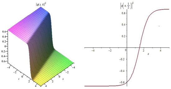
Figure 1. The profile of the dark soliton solutions (17).

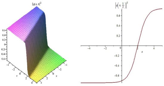
Figure 2. The profile of the dark soliton solutions (17).

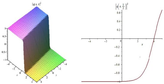
Figure 3. Shows the profile of the dark soliton solutions (17).

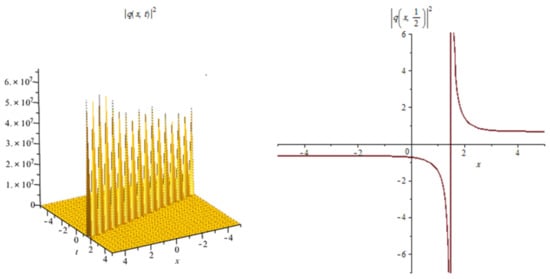
Figure 4. Shows the profile of the singular soliton solutions (19).

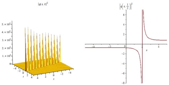
Figure 5. Shows the profile of the singular soliton solutions (19).

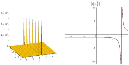
Figure 6. Shows the profile of the singular soliton solutions (19).

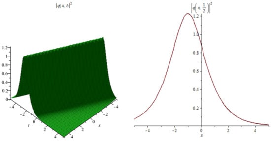
Figure 7. Shows the profile of the bright soliton solutions (29).

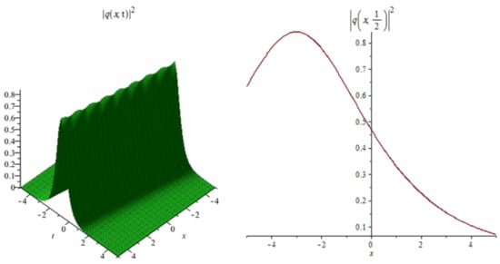
Figure 8. Shows the profile of the bright soliton solutions (29).

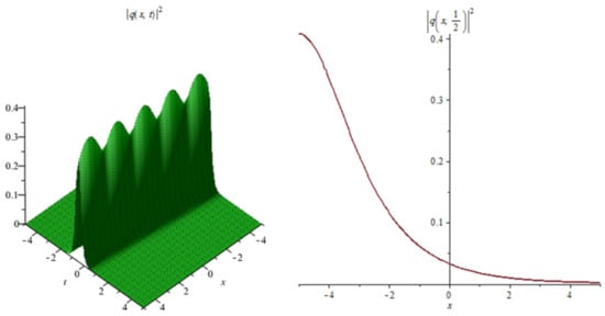
Figure 9. Shows the profile of the bright soliton solutions (29).

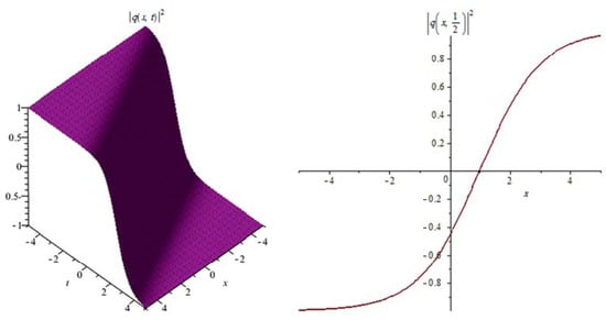
Figure 10. The profile of the combination of dark-bright soliton solutions (51).

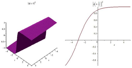
Figure 11. The profile of the combination of dark-bright soliton solutions (51).

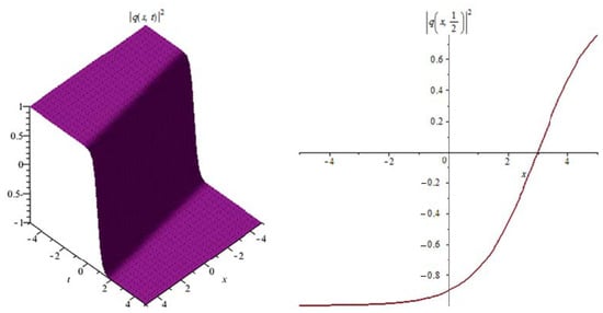
Figure 12. The profile of the combination of dark-bright soliton solutions (51).

Figure 13. The profile of the combination of bright-dark soliton solutions (55).

Figure 14. The profile of the combination of bright-dark soliton solutions (55).

Figure 15. The profile of the combination of bright-dark soliton solutions (55).

Figure 1: The numerical simulations of the solutions (17) 3D and 2D (with $t=\frac{1}{2}$) with the parameter values

$a_1=1,a_2=1,b=1,\sigma =0,\alpha =1,\kappa =2,w=2,\lambda =1,\mu =1,c=5,v=3,$$-5\le x,t\le 5.$

Figure 2: The numerical simulations of the solutions (17) 3D and 2D (with $t=\frac{1}{2}$) with the parameter values $a_1=1$, $a_2=1$, $b=1$, $\sigma =1$, $\alpha =1$, $\kappa =2,w=2,\lambda =1,\mu =1,$$c=5,v=4,$$-5\le x,t\le 5.$

Figure 3: The numerical simulations of the solutions (17) 3D and 2D (with $t=\frac{1}{2}$) with the parameter values $a_1=1$, $a_2=1$, $b=1$, $\sigma =2$, $\alpha =1$, $\kappa =2,w=2,\lambda =1,\mu =1,$$c=5,v=8,$$-5\le x,t\le 5.$

Figure 4: The numerical simulations of the solutions (19) 3D and 2D (with $t=\frac{1}{2}$) with the parameter values $a_1=1$, $a_2=1$, $b=1$, $\sigma =0$, $\alpha =1$, $\kappa =2$, $w=2$, $\lambda =1,\mu =1,$$c=5,v=3,$$-5\le x,t\le 5.$

Figure 5: The numerical simulations of the solutions (19) 3D and 2D (with $t=\frac{1}{2}$) with the parameter values $a_1=1$, $a_2=1$, $b=1$, $\sigma =1$, $\alpha =1$, $\kappa =2$, $w=2,\lambda =1,\mu =1,$$c=5,v=4,$$-5\le x,t\le 5.$

Figure 6: The numerical simulations of the solutions (19) 3D and 2D (with $t=\frac{1}{2}$) with the parameter values $a_1=1$, $a_2=1$, $b=1$, $\sigma =2$, $\alpha =1$, $\kappa =2$, $w=2$, $\lambda =1,\mu =1,$$c=5,v=8,$$-5\le x,t\le 5.$

Figure 7: The numerical simulations of the solutions (29) 3D and 2D (with $t=\frac{1}{2}$) with the parameter values $a_1=1,a_2=1,b=1,\sigma =0,\alpha =1,\kappa =\frac{1}{2},w=2,\lambda =1,\mu =1,$$c=5,v=-2,$$-5\le x,t\le 5.$

Figure 8: The numerical simulations of the solutions (29) 3D and 2D (with $t=\frac{1}{2}$) with the parameter values $a_1=1,a_2=1,b=1,\sigma =4,\alpha =4,\kappa =\frac{1}{4},w=16,\lambda =2,\mu =2,$$c=10,v=-6,$$-5\le x,t\le 5.$

Figure 9: The numerical simulations of the solutions (29) 3D and 2D (with $t=\frac{1}{2}$) with the parameter values $a_1=1,a_2=1,b=1,\sigma =2,\alpha =2,\kappa =\frac{1}{2},w=2,\lambda =1,\mu =1,$$c=5,v=-10,$$-5\le x,t\le 5.$

Figure 10: The numerical simulations of the solutions (51) 3D and 2D (with $t=\frac{1}{2}$) with the parameter values $a_1=4,a_2=2,b=-16,\sigma =0,\alpha =1,\kappa =2,w=10,\lambda =2,$$\mu =2,c=10,v=2,$$-5\le x,t\le 5.$

Figure 11: The numerical simulations of the solutions (51) 3D and 2D (with $t=\frac{1}{2}$) with the parameter values $a_1=4,a_2=1,b=-21,\sigma =1,\alpha =1,\kappa =2,w=24,\lambda =2,$$\mu =2,c=10,v=-6,$$-5\le x,t\le 5.$

Figure 12: The numerical simulations of the solutions (51) 3D and 2D (with $t=\frac{1}{2}$) with the parameter values $a_1=6,a_2=1,b=-16,\sigma =2,\alpha =1,\kappa =2,w=30,\lambda =2,$$\mu =2,c=10,v=6,$$-5\le x,t\le 5.$

Figure 13: The numerical simulations of the solutions (55) 3D and 2D (with $t=\frac{1}{2}$) with the parameter values $a_1=1,a_2=1,b=-16,\sigma =0,\alpha =2,\kappa =2,w=2,\lambda =2,$$\mu =2,c=10,v=-7,$$-5\le x,t\le 5.$

Figure 14: The numerical simulations of the solutions (55) 3D and 2D (with $t=\frac{1}{2}$) with the parameter values $a_1=1,a_2=1,b=-16,\sigma =1,\alpha =\frac{-5}{3},\kappa =2,w=2,\lambda =2,$$\mu =2,c=10,v=\frac{4}{3},$$-5\le x,t\le 5.$

Figure 15: The numerical simulations of the solutions (55) 3D and 2D (with $t=\frac{1}{2}$) with the parameter values $a_1=1,a_2=1,b=-16,\sigma =2,\alpha =2,\kappa =2,w=2,\lambda =2,$$\mu =2,c=10,v=-9,c_1=0,$$-5\le x,t\le 5.$

Let us now explain the effect of multiplicative white noise in the obtained solutions as follows:

In Figure 1, Figure 4, Figure 7, Figure 10 and Figure 13 when the noise $\sigma =0$, we note that the surface is less planer. But in Figure 2, Figure 3, Figure 5, Figure 6, Figure 8, Figure 9, Figure 11 and Figure 12 when the noise $\sigma$ increases ($\sigma =1,2,4$), we note that the surface becomes more planer after small transit behaviors. This means the multiplicative noise effects on the solutions and it makes the solutions stable.

8. Conclusions

In this article, we have obtained the solutions of the stochastic FLE in the presence of multiplicative white noise in the Itô sense. The modified simple equation method, the sine-cosine method, the Jacobi-elliptic function expansion method and the ansatze method are applied. Dark solitons, bright solitons, singular solitons, combo dark-bright solitons, combo bright-dark solitons, as well as Jacobi-elliptic solutions are given. Without noise ($\sigma =0$) the authors [1,2,37] studied a number of methods to get the exact solutions of FL equation while the stochastic FL Equation (1) is not yet studied. So, on comparing our stochastic solutions ($\sigma \ne 0$) obtained in our present article with the non- stochastic solutions ($\sigma =0$) obtained in [1,2,37] we deduce that the stochastic solutions are more general than the non-stochastic solutions. Finally, in future, this work will be extended in birefringent fibers, in fiber Bragg gratings and in magneto-optic waveguides. Also, we will study the stochastic FL Equation (1) with variable coefficients [37] when $\sigma \ne 0$, to get stochastic solutions.

References

- Biswas, A.; Yakup, Y.; Yaşar, E.; Zhou, Q.; Moshokoa, S.P.; Belic, M. Optical soliton solutions to Fokas-lenells equation using some different methods. Optik 2018, 173, 21–31. [Google Scholar] [CrossRef]
- Biswas, A. Chirp-free bright optical soliton perturbation with Fokas–Lenells equation by traveling wave hypothesis and semi-inverse variational principle. Optik 2018, 170, 431–435. [Google Scholar] [CrossRef]
- Albosaily, S.; Mohammed, W.W.; Aiyashi, M.A.; Abdelrahman, A.A.E. Excat solutions of the (2+1)-dimensional stochastic chiral nonlinear Schrödinger’s Equation. Symmetry 2020, 12, 1874. [Google Scholar] [CrossRef]
- Mohammed, W.W.; El-Morshedy, M. The influence of multiplicative noise on the stochastic exact solutions of the Nizhnik-Novikov-Veselov system. Math. Comput. Simul. 2021, 190, 192–202. [Google Scholar] [CrossRef]
- Mohammed, W.W.; Albosaily, S.; Iqbal, N.; El-Morshedy, M. The effect of multiplicative noise on the exact solutions of the stochastic Burger equation. Wave Random Complex Media 2021, 1–13. [Google Scholar] [CrossRef]
- Abdelrahman, A.A.E.; Mohammed, W.W.; Alesemi, M.; Albosaily, S. The effect of multiplicative noise on the exact solutions of Nonlinear Schrödinger’s Equation. AIMS Math. 2021, 6, 2970–2980. [Google Scholar] [CrossRef]
- Mohammed, W.W.; Ahmad, H.; Boulares, H.; Khelifi, F.; El-Morshedy, M. Exact solution of Hirota-Maccari system forced by multiplicative noise in the Itô sense. J. Low FrEquation Noise Vib Act. Control. 2021, 41, 74–84. [Google Scholar] [CrossRef]
- Zayed, E.M.E.; Alngar, M.E.M.; Shohib, R.M.A.; Biswas, A.; Yildirim, Y.; Alshomrani, A.S.; Alshehri, H.M. Optical solitons having Kudryashov’s self-phase modulation with multiplicative white noise via Itô Calculus using new mapping approach. Optik 2022, 264, 169369. [Google Scholar] [CrossRef]
- Zayed, E.M.E.; Shohib, R.M.A.; Alngar, M.E.M.; Biswas, A.; Moraru, L.; Khan, S.; Yildirim, Y.; Alshehri, H.M.; Belic, M.R. Dispersive optical solitons with Schrödinger-Hirota model having multiplicative white noise via Itô calculus. Phys. Lett. A 2022, 445, 128268. [Google Scholar] [CrossRef]
- Fokas, A.S. On a class of physically important integrable equations. Phys. D Nonlinear Phenom. 1995, 87, 145–150. [Google Scholar] [CrossRef]
- Jonatan, L. Exactly Solvable Model for Nonlinear Pulse Propagation in Optical Fibers. Stud. Appl. Math. 2009, 123, 215–232. [Google Scholar]
- Jonatan, L.; Fokas, A.S. On a Novel Integrable Generalization of the Nonlinear Schrödinger Equation. Nonlinearity 2009, 22, 11–27. [Google Scholar]
- Jonatan, L. Dressing for a Novel Integrable Generalization of the Nonlinear Schrödinger Equation. J. Nonlinear Sci. 2010, 20, 709–722. [Google Scholar]
- Kundu, A. Two-fold Integrable Hierarchy of Nonholonomic Deformation of the Derivative Nonlinear Schrödinger and the Lenells-Fokas Equation. J. Math. Phys. 2010, 51, 1–17. [Google Scholar] [CrossRef]
- Zayed, E.M.E. A note on the modified simple equation method applied to Sharma-Tasso-Olver equation. Appl. Math. Comput. 2011, 218, 3962–3964. [Google Scholar] [CrossRef]
- Jawad, A.J.M.; Petkovic, M.D.; Biswas, A. Modified simple equation method for nonlinear evolution equations. Appl. Math. Comput. 2010, 217, 869–877. [Google Scholar]
- Zayed, E.M.E.; Al-Nowehy, A.G. The modified simple equation method, the exp-function method and the method of soliton ansatz for solving the long-short wave resonance equations. Z. Naturforsch. 2016, 71, 103–112. [Google Scholar] [CrossRef]
- El-Borai, M.; El-Owaidy, H.; Arnous, A.H.; Moshokoa, S.; Biswas, A.; Belic, M. Dark and singular optical solitons with spatio-temporal dispersion using modified simple equation method. Optik 2017, 130, 324–331. [Google Scholar] [CrossRef]
- Arnous, A.H.; Ullah, M.Z.; Moshokoa, S.P.; Zhou, Q.; Triki, H.; Mirzazadeh, M.; Biswas, A. Optical solitons in birefringent fibers with modified simple equation method. Optik 2017, 130, 996–1003. [Google Scholar] [CrossRef]
- Arnous, A.H.; Ullah, M.Z.; Asma, M.; Moshokoa, S.P.; Zhou, Q.; Mirzazadeh, M.; Biswas, A.; Belic, M. Dark and singular dispersive optical solitons of Schrödinger-Hirota equation by modified simple equation method. Optik 2017, 136, 445–450. [Google Scholar] [CrossRef]
- Biswas, A. The tanh and the sine-cosine methods for the complex modified KdV and the generalized KdV equations. Comput. Math. Appl. 2005, 49, 1101–1112. [Google Scholar]
- Biswas, A. A sine–cosine method for handing nonlinear wave equations. Math. Comput. Model. 2004, 40, 499–509. [Google Scholar]
- Zayed, E.M.E.; Al-Nowehy, A.G. Solitons and other solutions for the generalized KdV-mKdV equation with higher-order nonlinear terms. J. Part. Diff. Equ. 2016, 29, 218–245. [Google Scholar]
- Yusufuglu, E.; Bekir, A.; Alp, M. Periodic and Solitary wave solutions of Kawahara and modifed Kawahara equations by using sine-cosine method. Chaos Solitons Fract. 2008, 37, 1193–1197. [Google Scholar] [CrossRef]
- Tascan, F.; Bekir, A. Analytical solutions of the (2 + 1)-dimensional nonlinear equations using the sine–cosine method. Appl. Math. Comput. 2009, 215, 3134–3139. [Google Scholar]
- Zayed, E.M.E.; Amer, Y.A.; Shohib, R.M.A. The Jacobi elliptic function expansion method and its applications for solving the higher order dispersive nonlinear Schrödinger’s equation. Sci. J. Math. Res. 2014, 4, 53–72. [Google Scholar]
- Liu, S.; Fu, Z.; Liu, S.; Zhao, Q. Jacobi elliptic function expansion method and periodic wave solutions of nonlinear wave equations. Phys. Lett. A 2001, 289, 69–74. [Google Scholar] [CrossRef]
- Xiang, C. Jacobi elliptic function solutions for (2+1)-dimensional Boussinesq and Kadomtsev-Petviashvilli equation. Appl. Math. 2011, 2, 1313–1316. [Google Scholar] [CrossRef]
- Lu, D.; Shi, Q. New Jacobi elliptic functions solutions for the combined KdV-mKdV equation. Int. J. Nonlinear Sci. 2010, 10, 320–325. [Google Scholar]
- Zheng, B.; Feng, Q. The Jacobi elliptic equation method for solving fractional partial differential equations. Abs. Appl. Anal. 2014, 228, 249071–249080. [Google Scholar] [CrossRef]
- Wazwaz, A.-M. New solitons and kink solutions for the Gardner equation. Commun. Nonlinear Sci. Numer. 2007, 12, 1395–1404. [Google Scholar] [CrossRef]
- Palencia, J.L.D. Travelling waves approach in a parabolic coupled system for modeling the behaviour of substances in a fuel tank. App. Sci. 2021, 11, 5846. [Google Scholar] [CrossRef]
- Jiao, Y.; Yang, J.; Zhang, H. Traveling wave solutions to a cubic predator-prey diffusion model with stage structure for the prey. AIMS Math. 2022, 7, 16261–16277. [Google Scholar] [CrossRef]
- Hu, Y.; Liu, Q. On traveling wave solutions of a class of KdV-Burgers-Kuramoto type equations. AIMS Math. 2019, 4, 1450–1465. [Google Scholar] [CrossRef]
- Bracken, P. The quantum Hamilton–Jacobi formalism in complex space. Quantum Stud. Math. Found. 2022, 7, 389–403. [Google Scholar] [CrossRef]
- Palencia, J.L.D.; ur Rahman, S.; Redond, A.N. Regularity and reduction to a Hamilton-Jacobi equation for a MHD Eyring-Powell fluid. Alex. Eng. 2022, 61, 12283–12291. [Google Scholar] [CrossRef]
- Gomez, C.A.; Roshid, S.H.O.; Inc, M.; Akinyemi, L.; Rezazadeh, H. On soliton solutions for perturbed Fokas–Lenells equation. Opt. Quantum Electron. 2022, 54, 370. [Google Scholar] [CrossRef]
- Nandi, D.C.; Safi Ullah, M.; Roshid, H.O.; Ali, M.Z. Application of the unified method to solve the ion sound and Langmuir waves model. Heliyon 2022, 8, e10924. [Google Scholar] [CrossRef]
Publisher’s Note: MDPI stays neutral with regard to jurisdictional claims in published maps and institutional affiliations. |
© 2022 by the authors. Licensee MDPI, Basel, Switzerland. This article is an open access article distributed under the terms and conditions of the Creative Commons Attribution (CC BY) license (https://creativecommons.org/licenses/by/4.0/).