Interference Mitigation for GNSS Receivers Using FFT Excision Filtering Implemented on an FPGA

Abstract

GNSS receivers process signals with very low received power levels (<−160 dBW) and, therefore GNSS signals are susceptible to interference. Interference mitigation algorithms have become common in GNSS receiver designs in both professional and mass-market applications to combat both unintentional and intentional (jamming) interference. Interference excision filters using fast Fourier transforms (FFTs) have been proposed in the past as a powerful method of interference mitigation. However, the hardware implementations of this algorithm mostly limited their use to military GNSS receivers where greater power and resources were available. Novel implementation of existing FPGA technology should make interference mitigation feasible with limited hardware resources. This paper details the practicalities of implementing excision filters on currently available FPGAs trading off the achievable performance against the required hardware resources. The hardware implementation of the FFT excision mitigation algorithm is validated with the GNSS software receiver. The results indicate that the desired performance of the developed algorithm has achieved the expectations and can provide significant improvement on mitigation techniques in current GNSS receiver hardware. Two hardware implementation designs (fixed-point and float-point data type format) are developed and compared to achieve the optimal design that can provide the best performance $\left(C/No\right)$ with the possible minimum hardware resources.

1. Introduction

Global navigation satellite system (GNSS) receivers are now embedded in our daily lives. The GNSS positioning, navigation, and timing (PVT) services have been used in multiple applications such as aviation, space, mapping, agriculture, military, and many other applications [1,2,3,4]. The rapidly increasing number of GNSS navigation services has resulted in demands for higher accuracy and increased receiver integrity and reliability. However, one key drawback of GNSS receivers is their vulnerability to a wide variety of interference signals within the GNSS frequency bands [5].

The definition of interference is a signal that lies within the GNSS band and out-powers the satellite signal, which in turn leads to difficulties in input decoding (jamming) or the induction of intentional false reading (spoofing). There are many types of interference sources including natural, man-made unintentional, and man-made intentional. Therefore, the most suitable noise characterization method is by bandwidth, which can be organized into two categories: narrrowband and broadband (wideband).

Jamming is the intentional interference by the emission of in-band electromagnetic radiations. This in turn blocks the GNSS signal, which is equivalent to a denial-of-service attack. It can use both narrrowband and wideband types of interference. One of the most popular jamming sources is the personal protection device (PPD), which is a jamming signal emitter that aims to disrupt the operation of nearby GNSS systems. Often, such devices are used in vehicles in order to hide their location. One such example is an accident that occurred in 2011 at the Newark International Airport. In November 2009, the local-area augmentation system (LAAS) of the airport installed a ground-based augmentation system (GBAS). However, this system was interrupted by the presence of radio-frequency interference. An investigation was launched and discovered the presence of jamming signals whose power exceeded more than 20 dB of the receiver antenna’s noise, resulting in tracking errors. After a lengthy investigation that reached two years, it was discovered that a truck driver was using a GPS jammer in order to hide the location of the vehicle. It turns out, however, that the jamming device used in this case was able to disrupt the operation of GNSS receivers within a radius of hundreds of meters. This led to the driver being fined more than 30,000 dollars [6,7,8,9]. Another incident occurred in Hong Kong in 2018, where more than 40 drones fell from the sky during a light show. The Hong Kong Tourism Bond’s Executive Director, Anthony Lau, stated that the reason was a GPS jammer [7,10]. In 2019, a jammer set up at a nearby pig farm was blamed for the intermittent GPS signal loss experienced by an aircraft landing at Harbin airport in north-eastern China. According to The South China Morning Post, the jammer was intended to stop criminal gangs from using drones dropping swine fever-infested packets on the herd, forcing farmers to sell them sick meat at a lower price [11]. In 2020, a French maker of high-precision GNSS technology claimed that GPS and Galileo signals were being frequently disrupted at their factory. After investigating, the French Radio Frequency Agency (ANFR) discovered the cause of the disturbance was a broadband router installed in a citizen’s adjacent flat. It was found that the malfunctioning router was producing detrimental interference at a frequency of 1581.15 MHz, which is very close to the GPS L1 and Galileo E1 signals at a frequency of 1575.42 MHz [12]. 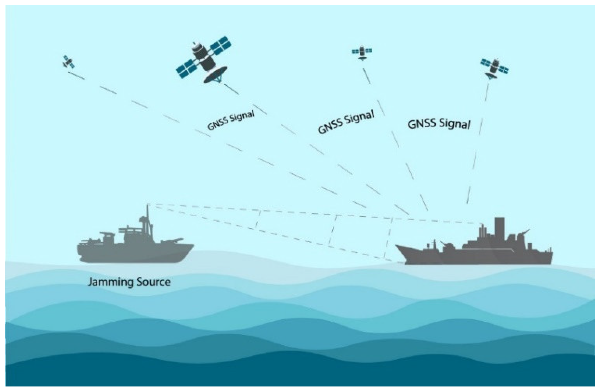Figure 1 shows the main concept of the jamming source interfering with an object such as a warship.

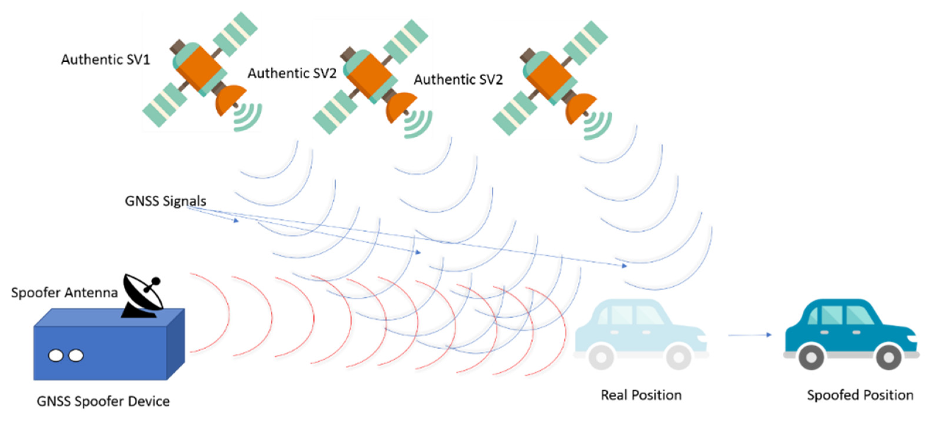
Spoofing, on the other hand, is an interference technique that records the real GNSS signal, modifies it, and emits it back as if it was the original signal. This in turn causes the GNSS receiver to make false readings. The re-emitted signal is far more powerful than the original and can easily mask it. Simpler spoofing devices simply change the phase of the GNSS signal, whereas more advanced devices can transmit a specific location. This does not directly cause any harm; however, systems that rely heavily on GNSS navigation can be compromised. This includes goods transportation. Some shipments are secured throughout their journey and are unlocked once the final destination is reached. In such examples, the security systems use the GNSS geo-location in order to identify the location of the load. Spoofing can interfere with the security system, allowing access to the shipment. Other applications such as autopilots use GNSS data for navigation and by spoofing the receiver and can steer the vehicle in the wrong direction. This is especially dangerous since military units such as drones rely on GNSS for navigation. Figure 2 shows a spoofing attack on the GNSS receiver.

The robustness of a GNSS receiver that has the capability to be protected from unintentional and intentional (jamming) interference is necessary to ensure reliability in GNSS services. Current GPS receivers have begun including anti-jamming algorithms that provide defence against jamming and unwanted interferences [13]. Current GNSS receivers have RF sections with automatic gain control (AGC) and multi-bit analogue-to-digital converters (ADCs) to provide protection against signal fluctuations and pulsed interference [14]. Moreover, the direct sequence spread spectrum (DSSS) is used in GNSS receivers to spread the received signal power over a wider bandwidth than the one used for information data. As a result, this spreading of the gain of the receiver reduces the effect caused by the narrowband interference [15].

However, these techniques are insufficient for applications such as military, aviation, and emergency services that require a high level of reliability. Over the past years, many researchers have detailed the interference effect and mitigations at different stages of the GNSS system, including antennas, low noise amplifier (LNA), AGC, intermediate frequency (IF), signal processing, and time-frequency domain techniques [16]. Interference increases the effect, which can be observed firstly in the receiver’s RF section, a decrease in AGC, and change in the distribution across ADC. When the interference power is too high, the available carrier-to-noise density ratio $\left(C/No\right)$ is reduced, degrading the performance of the receiver acquisition and tracking loops [14,17]. As the interference exceeds the GNSS systems’ anti-jamming ability, it will degrade the performance and ultimately result in the failure of the system.

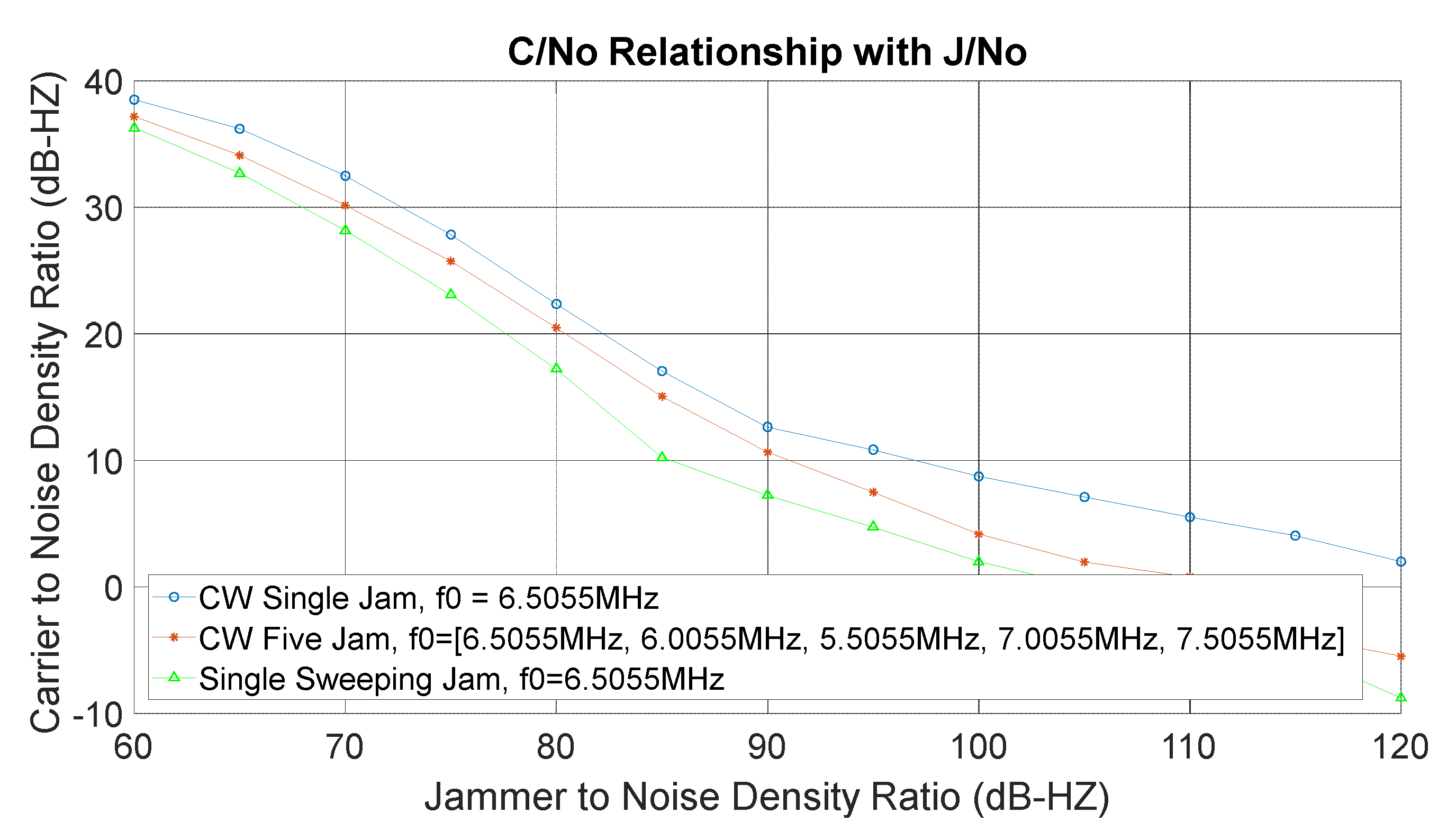
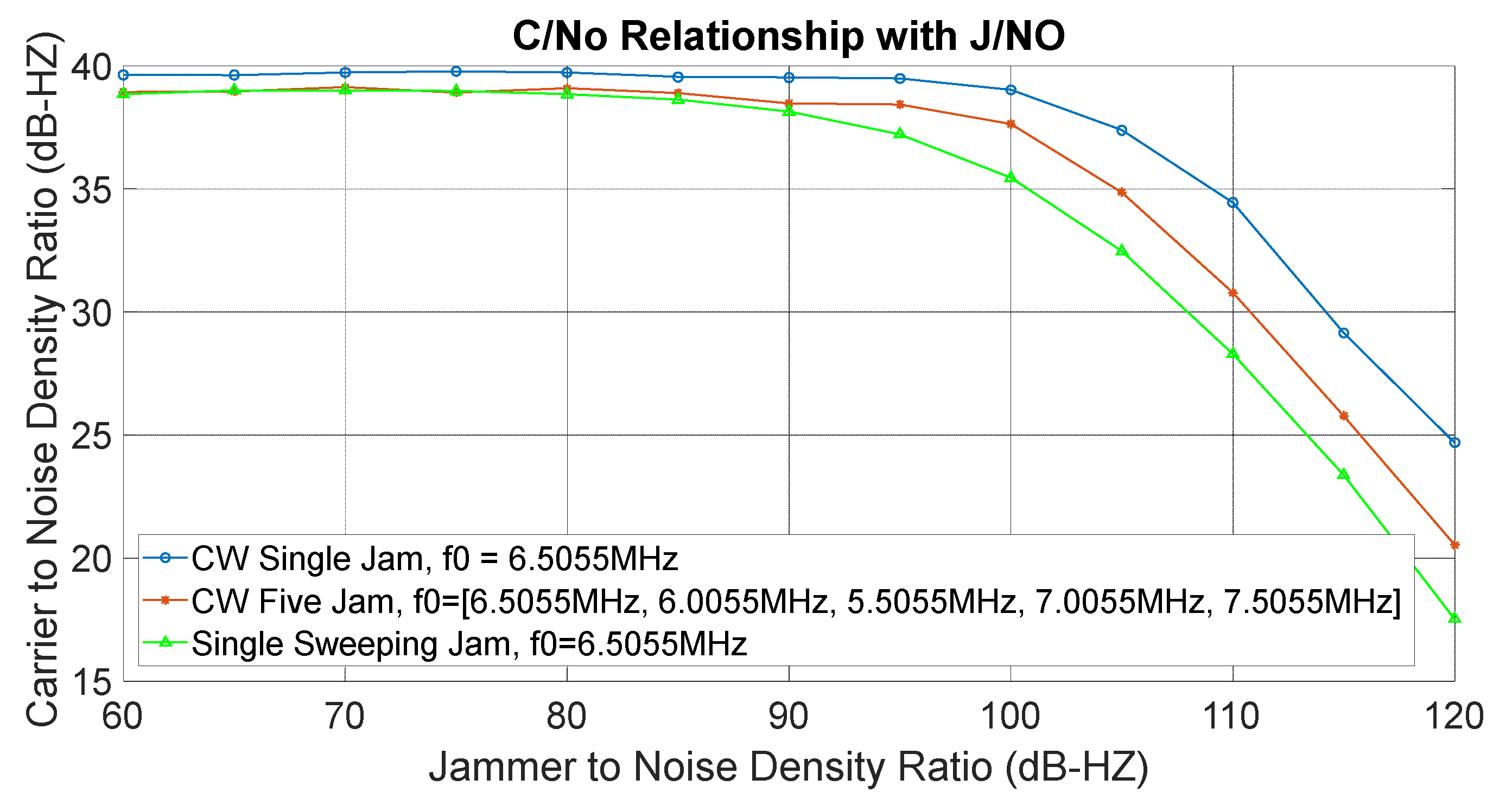
There are different types of interferences to be considered, broadly categorised into narrowband and wideband interference. This work addresses narrowband interference sources as wideband interference is generally addressed by multi-antenna beamforming techniques such as Novatel GAJT [18]. Within narrowband interference, continuous-wave interference (CWI), pulsed CWI, and sweeping interference are the most harmful interference impacting the quality of the received GNSS signals [17,19,20]. Therefore, CWI interference and sweeping interferences will be used in this research to illustrate the effect of the mitigation technique and compare it against other related techniques in the literature.

There is a huge array of algorithms that can improve the GNSS signal. Until recently, such devices were only discussed as theoretical solutions due to their computational costs. In this paper, the proposed interference excision filters were performed using fast Fourier transforms (FFTs), which were used as a powerful interference mitigation method. Furthermore, a novel hardware implementation for this mitigation technique was designed and tested using field programmable gate arrays (FPGAs), preserving the desired performance of GNSS receiver operations such as tracking, acquisition, and navigation against the required hardware resources. Moreover, a comparison between the results of the GNSS software receiver and the GNSS hardware implementation was conducted to demonstrate the proof of concept.

This interference mitigation algorithm was developed with a GPS L1 C/A signal generated by the front-end NSL Stereo at the intermediate frequency of 6.5 MHz, a 3 dB bandwidth of around 2.75 MHz, and frequency sampling at 26 MHz with a 2-bits resolution.

This paper is organized as follows. Section 2 reviews the recent related research on interference mitigation techniques for GNSS receivers. Section 3 illustrates the stages of developing the proposed FFT excision mitigation technique by discussing the MATLAB simulations. Section 4 demonstrates the VHDL hardware implementation stages. Section 5 discusses and evaluates the simulation results of the hardware implementation using VHDL and the validation stages. Finally, Section 6 concludes the paper.

2. Related Work

There has been a large amount of progress made not only in GNSS receiver technology but also regarding its application in which they perform relevant functions such as in the field of military, aircraft, maritime, space, and land applications. Furthermore, many studies have investigated the methods of mitigation of GNSS receiver interference. The aim of these studies is to remove or reduce the interference effects on the GNSS receiver and realise the desired carrier-to-noise density ratio $\left(C/No\right)$. As a result, receiver manufacturers and researchers have investigated different kinds of GNSS interference mitigation techniques.

The first and most widely used method is an adaptive notch filter. A notch or bandstop filter is a good choice for mitigating CW interference in the passband of the GNSS signals. This sort of interference is generally either self-generated or from a fixed source nearby such as a transmitting antenna. Analogue notch filters can be applied at the RF path or digital filters can be employed at the sampled IF signal to provide more flexibility. An adaptive notch filter is able to detect the centre frequency of the interference and adjust the notch filter to match. This can provide a trade-off in terms of power consumption and processing power [21,22,23]. The authors in [24] present two frequency lock loop (FLL) equivalent models of an adaptive notch filter to detect sweeping jammers: one is standard and the second one is exponential filtering FLLs. They showed that the standard FLL has a better performance regarding the interference than the FLL exponential filter. This research work was extended in [25] by the proposal of an FLL-equivalent adaptive notch filter (ANF) to mitigate different types of interference. The ANF process consists of three parts. The first part is the adaption unit, which estimates the centre frequency to be removed. The second part is the detection unit, which decides whether to remove any narrowband interference. The third part is the notch filter, which is activated by the detector to process the input signal by suppressing a narrowband frequency around the rejected frequency set by the adaption unit. The drawback of this study is the power consumption issue, as the proposed detection method is based on the output-input power ratio. This detection method results in high-power consumption being efficient for interference mitigation; the stronger the interference is, the higher the suppression power that is required. In [13], the estimation of the jammer’s frequency band is performed with a Prony estimator instead of FFT/IFFT in order to decrease the complexity of the whole algorithm. The adaptive notch filter shows small performance improvements (~10 dB) at the level of interference that can be tolerated with sweeping continuous-wave (CW) interference. This small improvement is due to the relatively simple implementation of using one or two-pole notch filters, which can only achieve a very limited depth in the null of the notch filter. Similar levels of mitigation can be seen in mass-market receivers as investigated in [13]. They considered a low level of interference while this paper aimed to achieve greater levels of resistance to interference using higher-order filtering.

The second method is empirical mode decomposition (EMD) and blind source separation (BSS) [26]. In this method, the signal is decomposed iteratively by interpolating the min and max of the signal and removing this interpolated signal from the original signal. The work published in [26] developed two-stage algorithms. In the first stage, EMD is used to find the pseudo-periodic signals amid the received signal. This works well for stationary signals. However, nonstationary signals are more complicated, and the use of a second stage is required. The second stage is a blind source separation algorithm (or BSS). The drawback of this stage is that BSS is a complex algorithm (e.g., matrix inversion, determinant), hence requiring a large number of computations. Moreover, this method works with jamming to signal power ratios (JSRs) of up to 45 dB with nonstationary jamming. However, the method starts to be degraded at 50 dB [26]. To overcome this issue, a suggested solution has been discussed of combining spatial filtering with this technique [27,28]. Another solution is to integrate the Kalman filter with this algorithm to estimate the phase/code delay. As a result, this combination may enable processing in the presence of a stronger or higher level of jamming [26].

The third method is the wavelet filter. Recently, wavelet filters have been implemented to mitigate interference in GNSS as proposed in [29,30]. In these references, interference detection is achieved through a time-scale representation of the GNSS-interfered received signal exploiting the wavelet functions. The wavelet transform provides decomposition of a signal by taking advantage of a group of orthogonal local basis functions [30]. The suppression is observed by the threshold in each wavelet scale. Each coefficient of the wavelet packet decomposition is compared to a predetermined threshold, and it is blanked or clipped when such a threshold is exceeded. Threshold determination is performed according to the required false alarm probability and a statistical characterization of the GNSS signal obtained in an interference-free environment [29]. However, the results are not compelling, and a wavelet filter would only be suitable for specific high-grade receivers because of the processing time and high complexity.

The fourth method is zero-memory non-linearity. This algorithm, which is also called complex signum non-linearity, is another statistical approach, derived from the Laplace distribution. These techniques mitigate the interference by generalising the correlation process. This is achieved by extracting the sign of each sample, resulting in +1 for positive values and −1 for negative values. The major advantage of this algorithm is that no signal estimation is required as it is often the weak point in many interference mitigation techniques. This also implies that no settings are required for the optimal operation of the filter. In addition, the algorithm is relatively efficient when it comes to computational costs. In fact, it only works if part of the samples is affected by the interference (pulsed jamming); therefore, it cannot mitigate continuous jamming [31].

The fifth method is pulse blanking, which is a widely used technique in mitigating the pulsed interference of GNSS receivers due to its simplicity and effectiveness. Pulse blanking (PB) uses the zeroing techniques of the received signal sample that is affected by the interferences [32]. PB is a pre-correlation mitigation technique and it is applied to the down-converted signal before the correlation process. The disturbing signal is removed by zeroing the samples corrupted by the interference pulses. In order to accomplish this, it is important to determine the pulse position. The techniques that are used to estimate the pulse position are ideal blanking and thresholding [32]. However, this method works with a combination of automatic gain control (AGC). AGC should be reduced in the case of no existing interference. Otherwise, this technique will remove parts of the original signal. This technique can be used in combination with other techniques to address the specific problem of pulsed interference.

The sixth method is the fast Fourier transform (FFT) filter. FFT excision is a powerful tool for detection and interference removal. The ability to modify the received spectrum allows for rapid and efficient removal of jammers with different characteristics (bandwidth, frequency, pulsed, sweeping rate) compared to other algorithms [33,34]. Additionally, it has the ability to act on multiple jamming sources and can even be used as an equalization filter of the receiver’s RF front-end biases. The performance of transform domain interference suppression in GNSS receivers based on fractional Fourier transform (FrFT) with an adaptive threshold was presented in [34]. However, the limitation of their proposed algorithm is the adaptive selected threshold, which was unable to handle a wide bandwidth of interference. As a result, this distorts the desired signal when spectral components suppress the interference. The results of the proposed algorithm worked with up to 45 dB (J/No) of the CW jammer. On the other hand, our proposed FFT mitigation algorithm works with wideband interference and the results demonstrated that our algorithm has the capability to suppress more than 100 dB (J/No) of the CW jammer without distortion of the original signal. The disadvantage of the FFT excision has been related to the complexity of the implementation in the receiver hardware. However, efficient computation of FFTs is now common in almost all receiver architectures and possible in low-power ASICs for the mass-market [35]. The hardware implementation of interference mitigation using FFT algorithms has not been extensively explored in the literature. It can be deduced from the literature review that the current studies have focused on interference mitigation algorithms in terms of software simulations and only a few studies have focused on hardware implementations. In [36], the authors proposed a high-rate DFT-based data manipulator (HDDM) algorithm with different FPGA-based GNSS dual-band receivers. These receivers were pre-selected based on the number of bits ADC. They used 4, 8, and 14 bits ADC. This algorithm only works against the pulsed interference, with suppression of 50 dB JSR. However, HDDM has shown disappointing results for simple CW interference due to its limited selectivity of frequency and limited robustness of HDDM. The authors mentioned that to overcome this challenge, a notch filter has to be combined with the HDDM algorithm. This research work is extended in [37] by suggesting HDDM with AGC instead of pulse blanking (PB) to overcome the challenge of removing parts of the signal in the presence of wideband noise interference. HDDM-AGC has real-time FPGA implemented on a wideband receiver. The limitation of this study is the test setup by 1-bit DAC used by the R&S up-converter. This introduces a significant quantization loss, which results in a $\left(C/No\right)$ loss of 6 dB.

Therefore, the main aim of this paper was to assess the complexity and feasibility of the FFT excision filter implementation in current FPGA technology. Additionally, we aimed to overcome the challenges encountered in the previous research. The proposed FFT excision filter algorithm has the capability to work with different types of GNSS interference such as narrrowband interference, wideband interference, CW interference, pulsed CW interference, and sweeping interference. The estimation of jammer characteristics often requires FFT even if a different technique is used for interference removal. Compared to the EMD and wavelet filter, they have not convincingly shown better performance results than the FFT excision filtering algorithm. Additionally, the complexity is expected to be much higher due to their high computing requirements, so they were not considered for hardware implementation. For these reasons, FFT excision filtering was used in this research work to mitigate the influence of interference on the GNSS receiver and enhance its performance for tracking and navigation operations. The proposed interference mitigation algorithm demonstrated a significant performance improvement $\left(C/No\right)\cong 40\mathrm{dB})$ compared to other algorithms, developed in the software simulations, and implemented in FPGA hardware.

3. Proposed Methodology

This research methodology is based on quantitative research methods. The quantitative methods are presented using experimental research methodology and engineering-oriented research methodology.

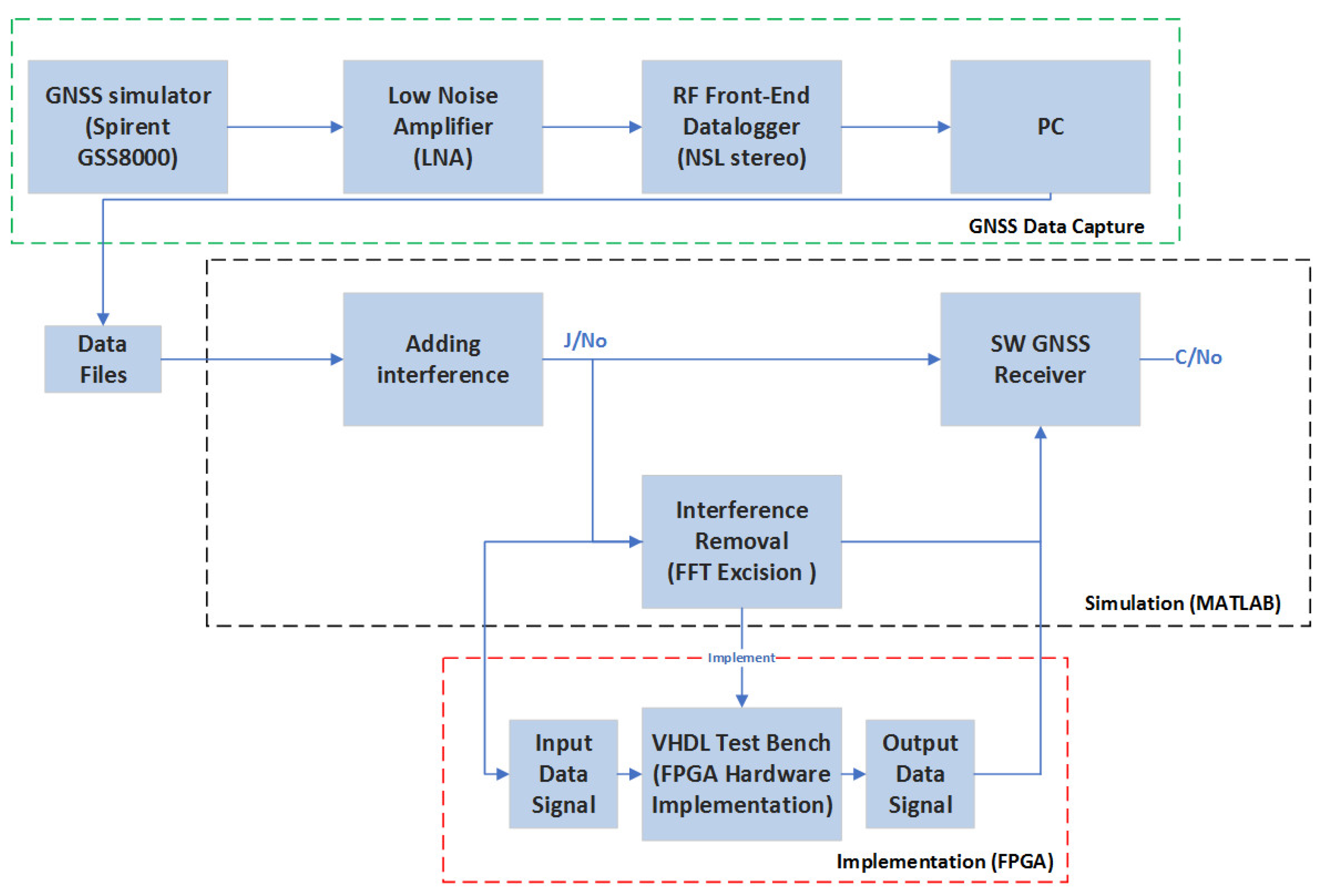
Figure 3 shows the full scheme of the proposed methodology and experimental work for this research. This research work consists of three stages as shown in Figure 3, which are GNSS data capture, MATLAB simulation, and FPGA implementation. The first stage is called GNSS data capture. The first block of this stage represents the GNSS simulator (Spirent GSS8000), which produces representative GNSS signals whose power levels can be controlled as desired. The output of the simulator represents the RF GNSS signal at the output of the receiver’s antenna. It is then amplified using the low noise amplifier (LNA). LNA is a fundamental component because it amplifies the signal that comes from the antenna without adding a significant level of noise. This boosts the signal to protect it from the noise sources generated within the system (switching noise, harmonics, etc). The next block is the RF front-end datalogger. This block has two phases. Regarding the first phase, the RF signal is converted to an intermediate frequency (IF) that has a sufficient frequency to support the signal bandwidth. The second phase is the signal being converted to digital signals using an analogue digital converter (ADC) with automatic gain control (AGC). The output digital IF is passed to PC and stored as a data file. The second stage is the simulation and testing of the GNSS receiver performance using MATLAB. This stage contains three main blocks, which is the addition of interference, interference mitigation (the FFT excision), and the software GNSS receiver. The narrowband interferences that can be applied are single jammer, multiple jammers, and sweeping jammers, all with configurable power levels and frequencies. After this, the data is sent to the interference removal filter block, which represents the designed FFT excision filter, to mitigate the GNSS receiver interference. Finally, the signals are sent to the software GNSS receiver after the interference mitigation to test the influence of the jamming on the receiver operations.

The fundamental stage of this research is the third stage, which is the implementation stage in FPGA. This stage is carried out for both the hardware implementation and to validate the simulation and testing stage. As shown in Figure 3, the output signal data with the added interference acts as an input for the very high-speed integrated circuit hardware description language (VHDL) test bench. Then, the output of the VHDL test bench is verified by sending it back to the software GNSS receiver to test the performance and compare it with the MATLAB simulation results. Using this comparison algorithm, the FFT excision-designed filter is verified as an optimal solution to mitigate the interference of the GNSS receiver in terms of software simulation and hardware implementation. The following sections illustrate the stages of developing the proposed scheme.

3.1. Scenarios: Different Types of Interference

This scheme was evaluated using different scenarios that have been discussed according to the related works in [13,38,39]. There are main parameters for each scenario, which are the centre frequency ($f_0$) of the jamming signal, the intermediate frequency ($IF$) of the jamming signal, and the jamming to noise density ratio ($J/No$). The centre frequency ($f_0$) is a measure of the centre frequency between the upper and lower cut-off frequency. The centre frequency is relative to the RF front-end’s intermediate frequency ($IF$). The intermediate frequency ($IF$) is a frequency in which a carrier wave is shifted as an intermediate step in transmission or receiving. In this work, $IF$ was selected to be 6.5 MHz and the jamming to noise density ratio ($J/No$) increased with the amplitude of the jamming signals. The applied jamming interferences in the simulation were continuous-wave (CW) interference and the sweeping frequency jammer.

Table 1. The considered interference scenarios for evaluating the scheme.

Scenarios	Number of Jammers	Jammer Centre Frequency, ${\mathit{f}}_0$ (IF = 6.5 MHz)	Frequency Sweep Rate	$\mathbf{Jamming}\mathbf{Levels}(\mathit{J}/\mathit{N}\mathit{o})$
Scenario 1	One Jammer	−5.5 MHz to 7.5 MHz	0 Hz	0 to 130 dB-Hz
Scenario 2	Multiple Jammers (2 to 10)	−5.5 MHz to 7.5 MHz (equally spaced across the band)	0 Hz	0 to 130 dB-Hz
Scenario 3	(Sweeping Frequency)	−5.5 MHz to 7.5 MHz	0 to 20 GHz/s	0 to 130 dB-Hz

shows the parameters of these scenarios carried out in this work. The first scenario was simulated using one continuous-wave jammer that had a centre frequency ($F_0$) at 6.5 MHz and the interval frequency was between −1 and 1 MHz with a jamming to noise ($J/No$) ratio from 0 to 130 dB-Hz. The second scenario was simulated using multiple continuous-wave jammers with the same parameters as the first scenario. We followed the same approach in [13,39] to simulate the frequency fixed jammer to achieve the first and second scenarios using the following Equation (1):

$$J\left(t\right)={\sum }_{i=0}^{p}A\sin \left(2\pi \left(f_0+d{f}_i\right)t\right)$$

(1)

where p is the number of jammers (equal to one in the first scenario and equal to 2 or 3 or a higher number than 1 in the second scenario). $f_0$ is the centre frequency and $d{f}_i$ is the change in the frequency due to the interval. $\left(f_0+d{f}_i\right)$ is included in the interval [5.5–7.5] MHz as mentioned in Table 1. The jamming signal amplitude increases with ($J/No$) in the simulations. However, the amplitude does not vary between multiple jammers in the same simulation file and the phase of the jammer is omitted from this definition and set to zero in our simulations. 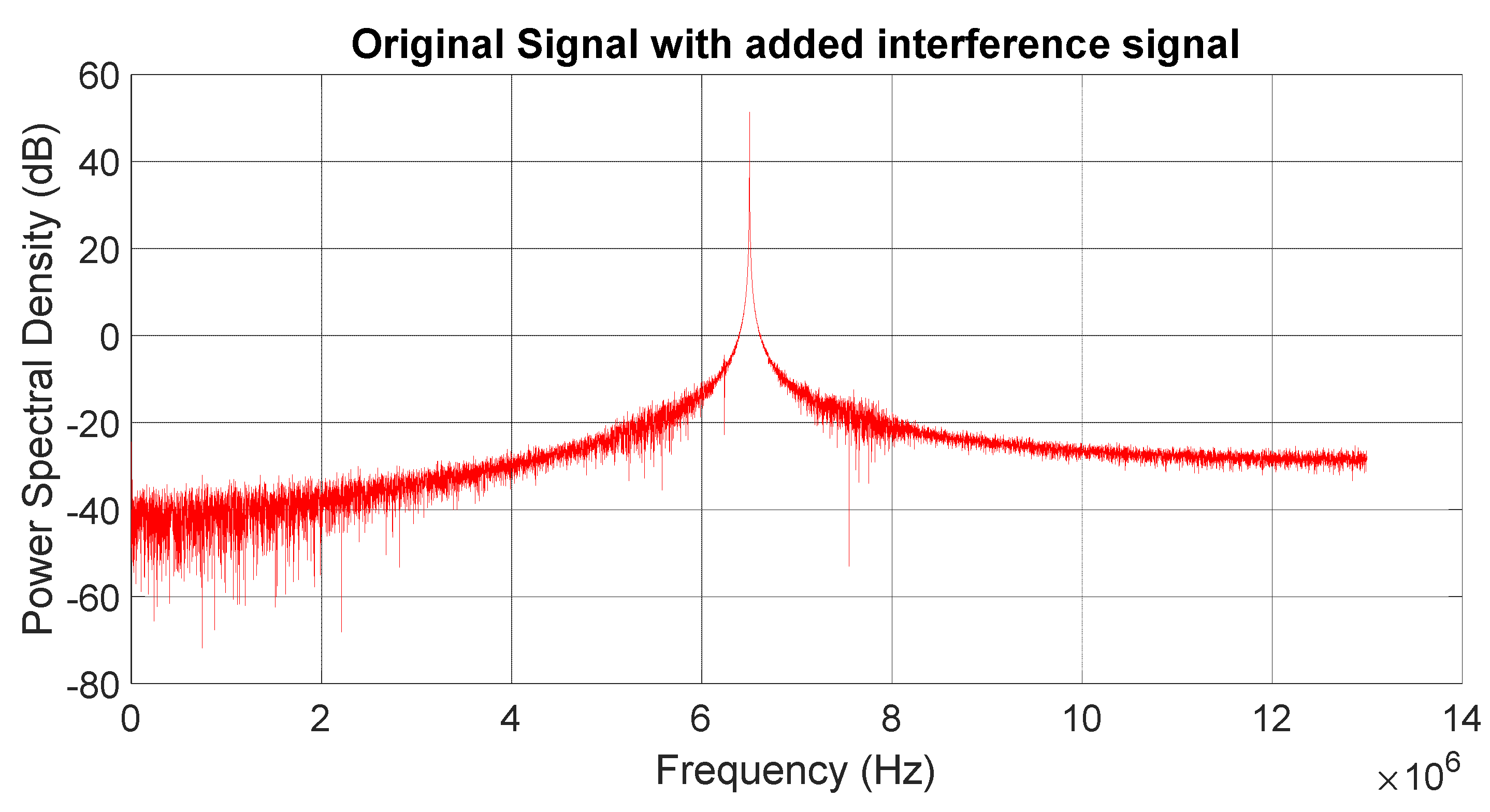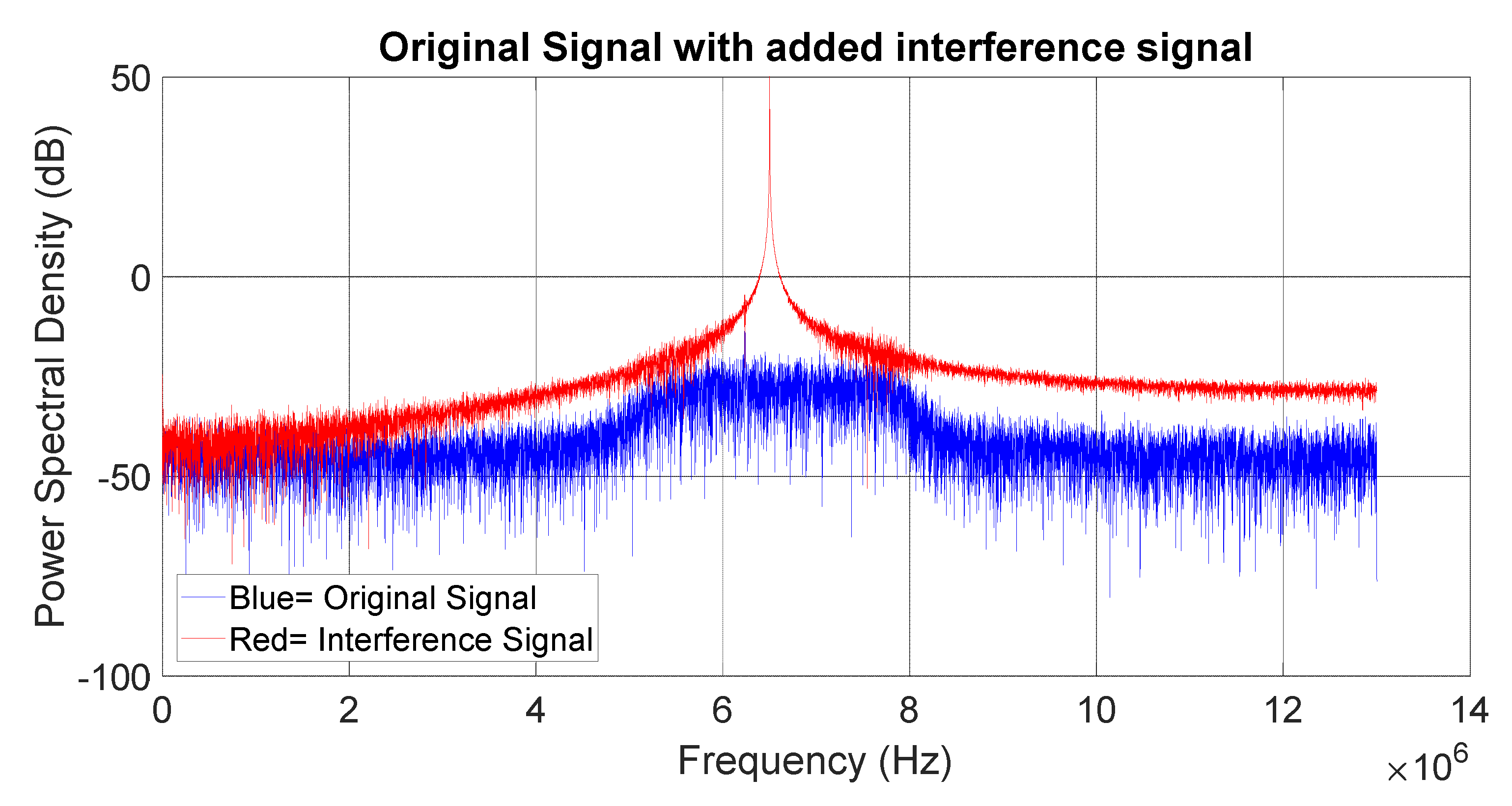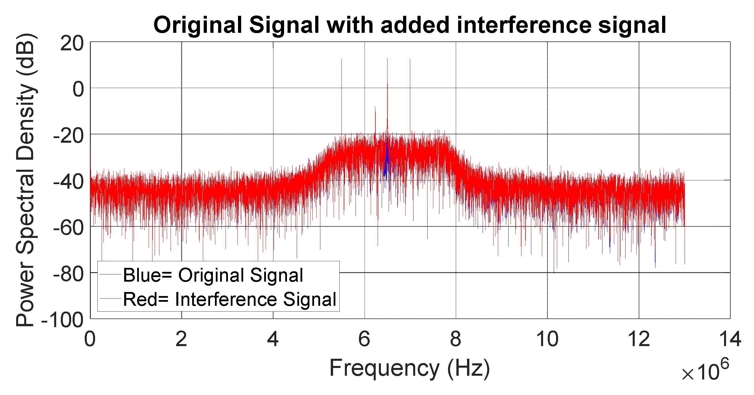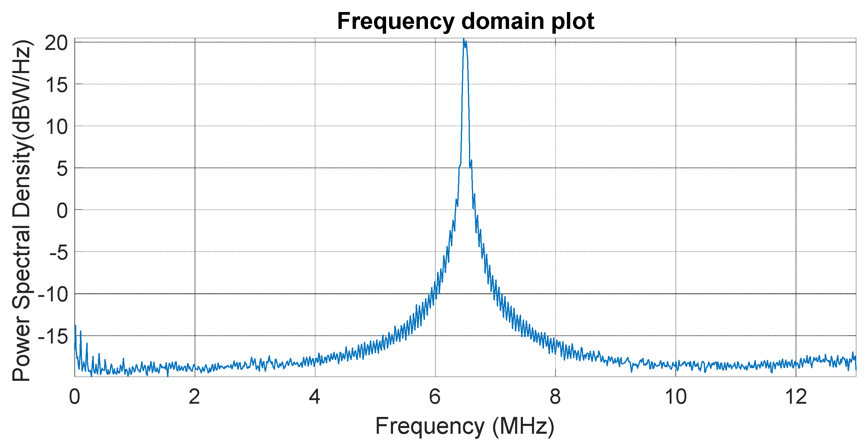Figure 4 shows an example of a continuous-wave jammer at ($J/No$) = 80 dB-Hz.

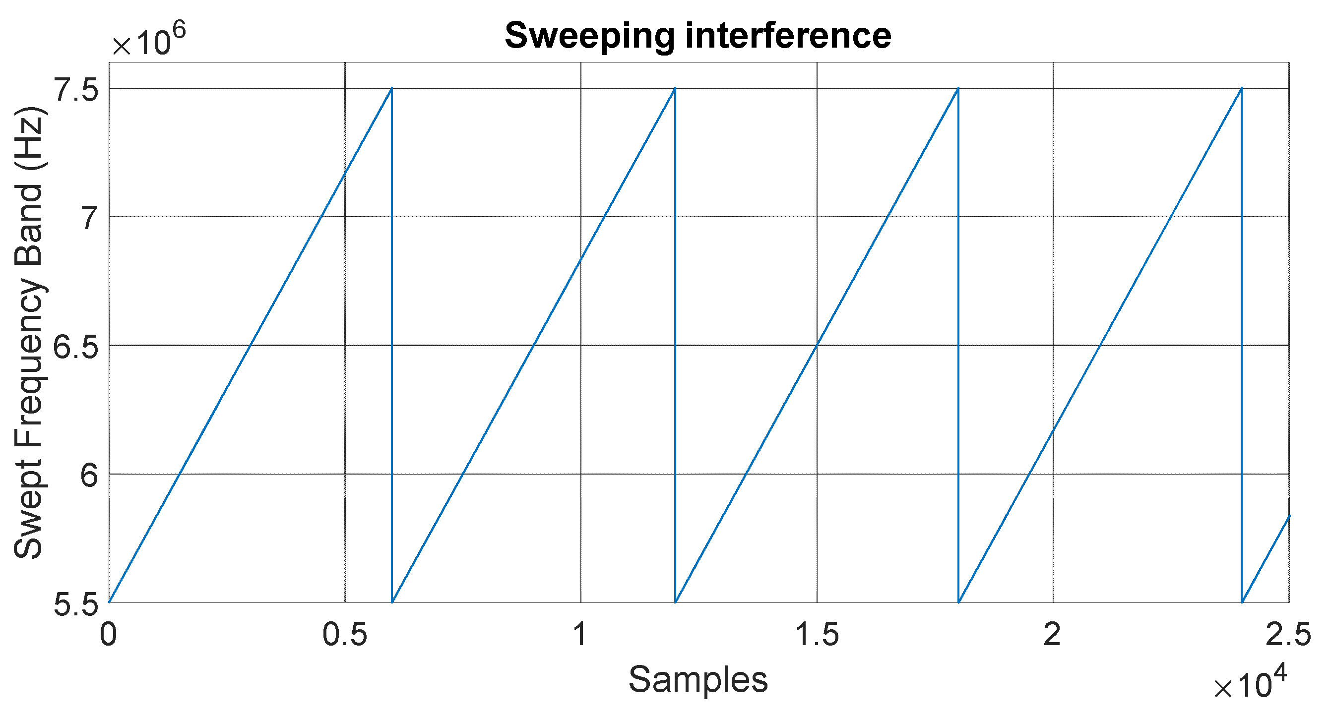
The third scenario was simulated using a sweep jammer that had a certain frequency of 6.5 MHz and the swept bandwidth was −1 to 1 MHz with a jamming to noise ratio from 0 to 130 dB-Hz and the frequency rate was set to 8.4 GHz/s for a comparison with the results given in [13]. The sweeping frequency jammers were defined with the following Equation (2):

$$J\left(t\right)=A \sin \left(2\pi \left(f_0+d{f}_i\left(t\right)\right)t\right)$$

(2)

where $df\left(t\right)$ is a time-varying frequency offset. Figure 5 shows an example of the frequency variation of a jammer sweeping at a sweeping rate of 8.4 GHz/s (with a sampling frequency of 26 MHz).

3.2. Degradation of the GNSS Receiver Performance

There are various ways to monitor the degradation of GNSS receiver performances. The first way is at the signal level (i.e., bit error rate, carrier-to-noise ratio, monitoring phase/frequency lock loop, saturation phenomenon of AGC). The second way is at the observation level (i.e., noise on pseudoranges and carrier-phase observations) or the navigation level (i.e., position accuracy).

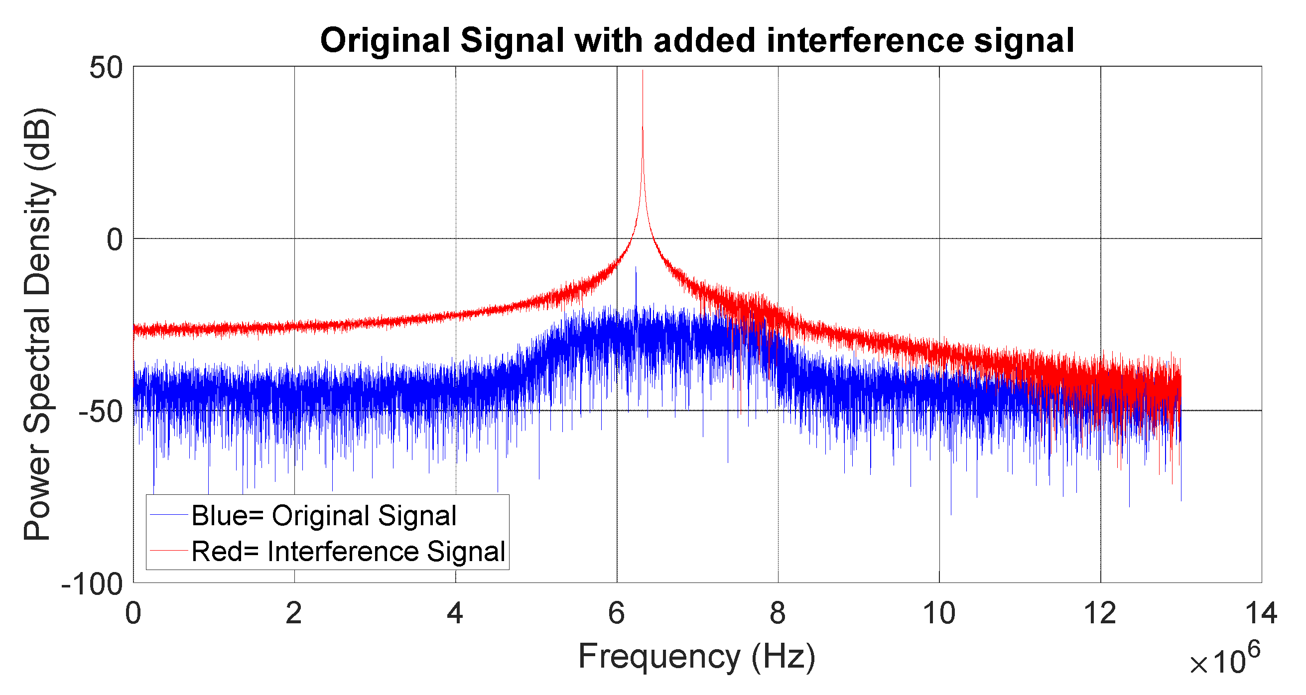
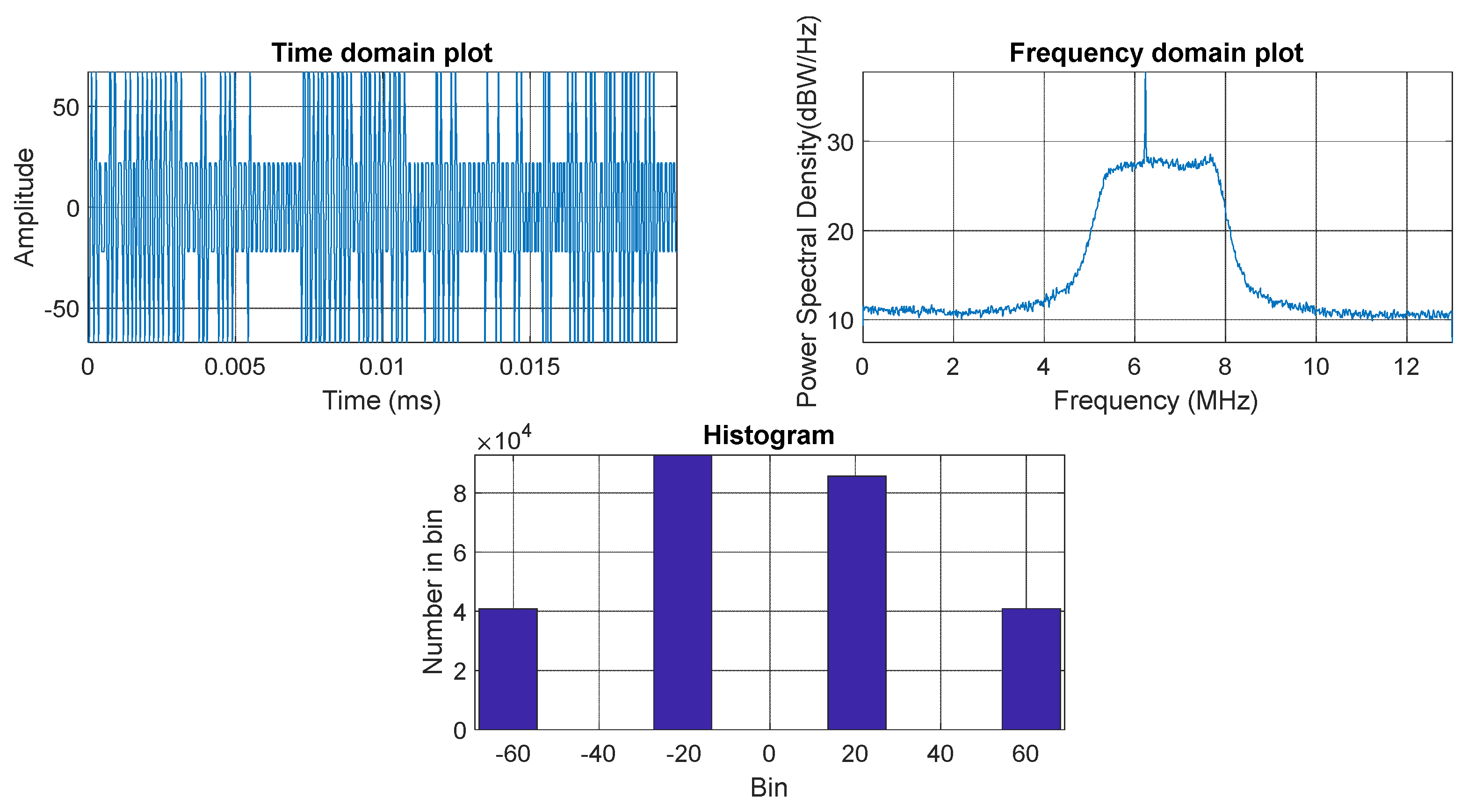
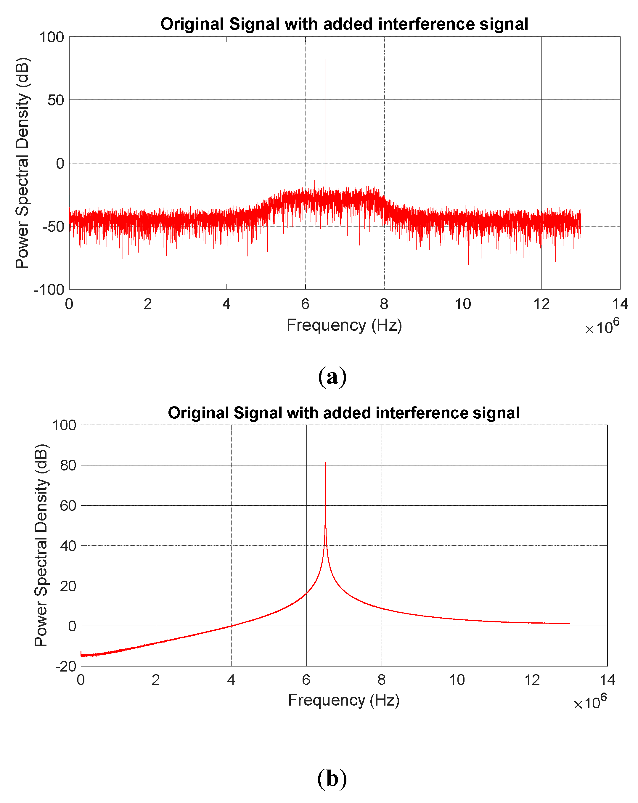
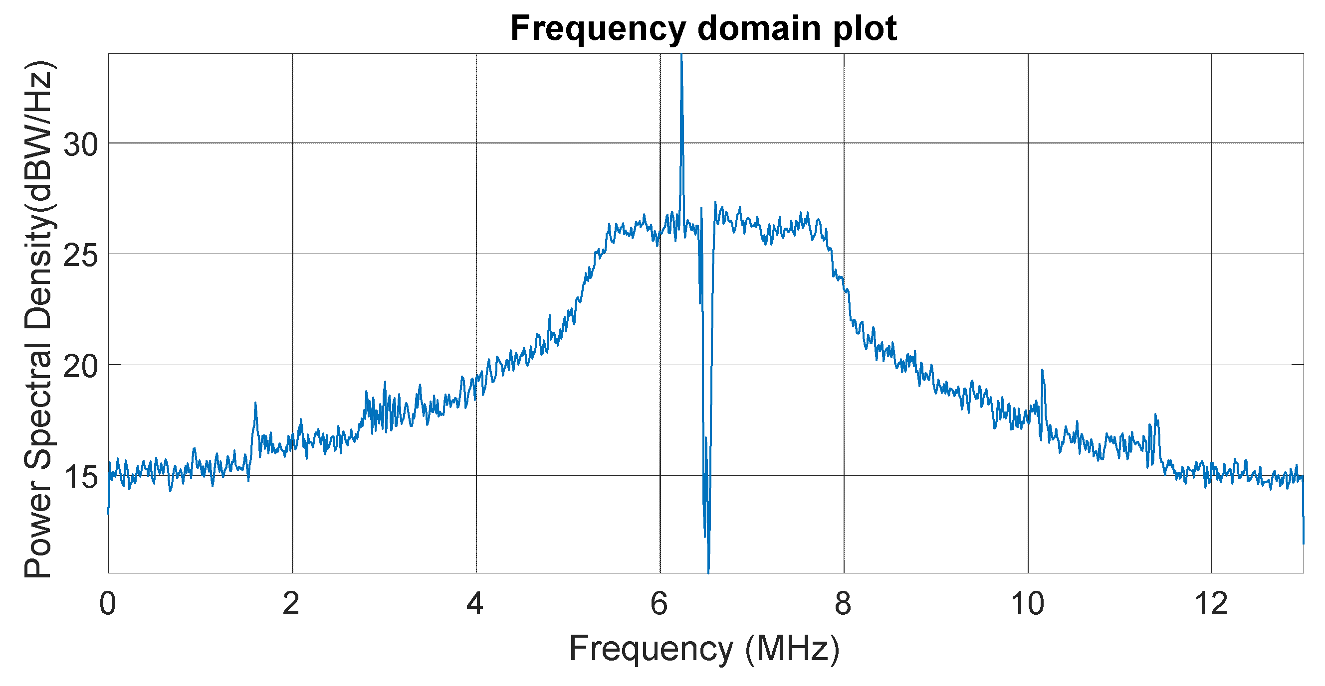
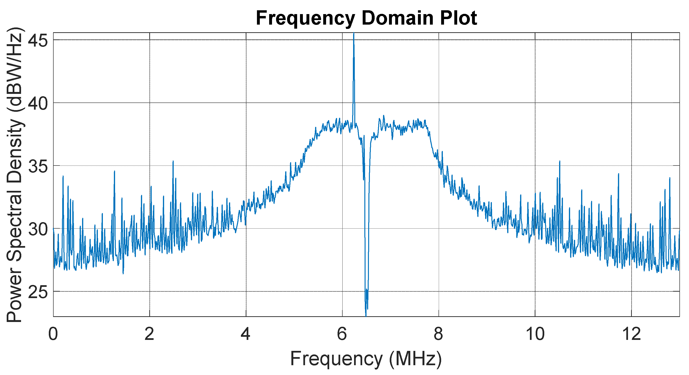
The first step for the simulations and experiments was the collection of the raw data. The raw data was logged for a typical terrestrial scenario, with all GNSS satellites set to a power level of −130 dBmW. The reason behind this power level is that the minimum received power level of GPS L1 C/A code (signed used) is −128.5 dBmW (from IS-GPS-200-M), assuming a 3 dBi receiver antenna. Therefore, −130 dBmW is slightly conservative but reasonable for a low-cost antenna. The power spectral density and bit distribution of the sampled signal is shown in Figure 6. It illustrates the raw data before the addition of the interference in three different representations, which are the frequency domain, the time domain, and the histogram representations. The sampling frequency, IF, and bandwidth used were determined by the utilized GNSS front end, which is defined by the GNSS datalogger (NSL Stereo). The interference frequencies were chosen to be in line with [13,20] to provide a comparison against the notch filter approach, which is widely used in mass market receivers. The front end was configured to down-convert the GPS L1 C/A signal to an intermediate frequency ($IF$) of 6.5 MHz, with a 3 dB bandwidth of around 2.75 MHz and frequency sampling at 26 MHz with a 2-bits resolution. It is noticeable that there is a self-generated CW in-band at 6.235 MHz, 10 to 12 dB above the noise, but it is not strong enough to interfere with the GNSS tracking after the matched filter of the spreading code demodulation was applied. The RF data was quantized to 2 bits during logging. As shown in Figure 6, the time domain’s amplitude fluctuated between negative and positive values. The signal was heavily quantised down to 2 bits, taking on values of (±1, ±3). This is common in GNSS receivers, where the long averaging times result in only a 0.5 dB impact on SNR for 2-bit quantisation. However, in the simulation, we allowed 8 bits of the ADC range to handle the interference. To simulate the automatic gain control of the RF front-end, the standard deviation of the signal was always adjusted to around one-third of the signed 8-bit range ($128/3\cong$ 42). The 8-bit signed has 7 bits of data and one bit of the sign $(2^7=128)$.

3.3. Mitigation Algorithm (FFT Excision)

The proposed solution for interference mitigation is the FFT excision algorithm. In its most simple form, FFT excision is the process of converting the signal into the frequency domain via FFT, selecting the frequency bins to be removed, and then performing an inverse FFT to return the signal to the time domain for processing by the receiver’s acquisition and tracking routines. However, as we demonstrate, this process can result in the removal of large amounts of the received spectrum for certain jammer frequencies. The frequency bin resolution is an important term for determining the location of the centre of interference in the spectrum. The frequency resolution is the difference in the frequency between each bin, and thus sets a limit on how precise the results can be. The frequency bin resolution (FBN) is calculated as in Equation (3):

$$Frequencybinresoultion \left(FBN\right)=\frac{\mathrm{Fs}}{FFTlength}$$

(3)

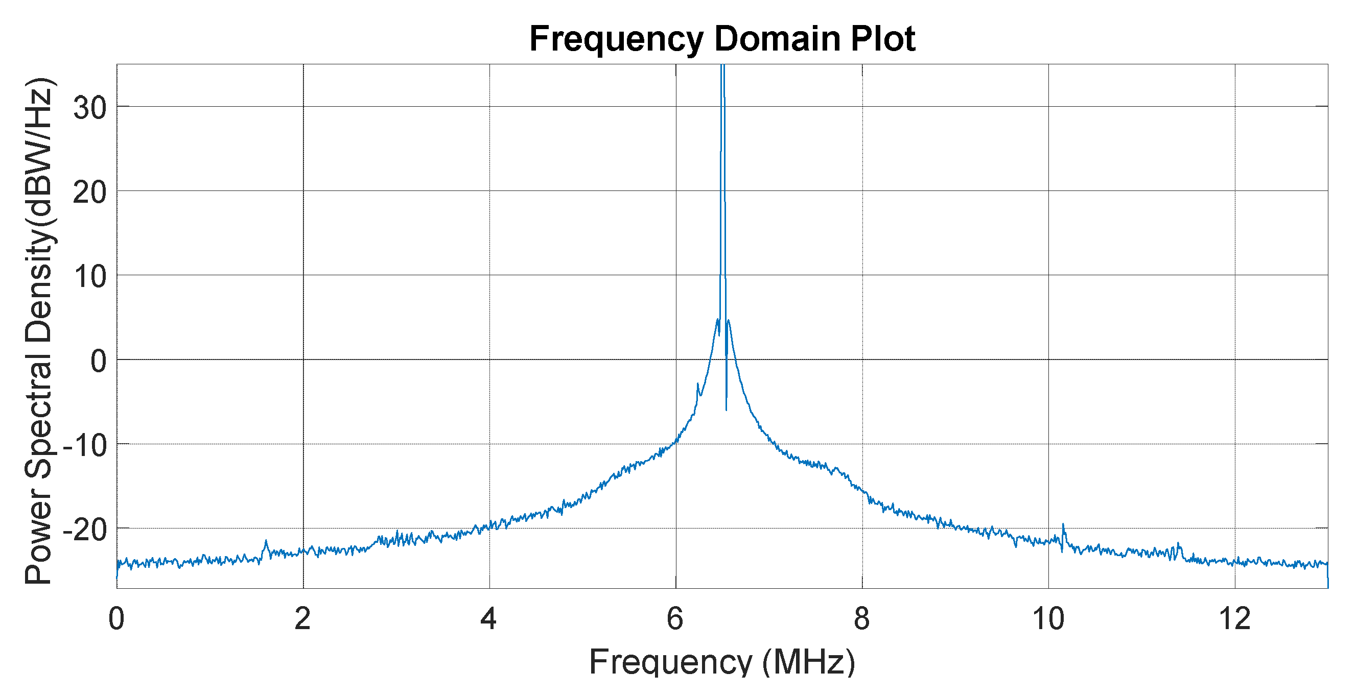
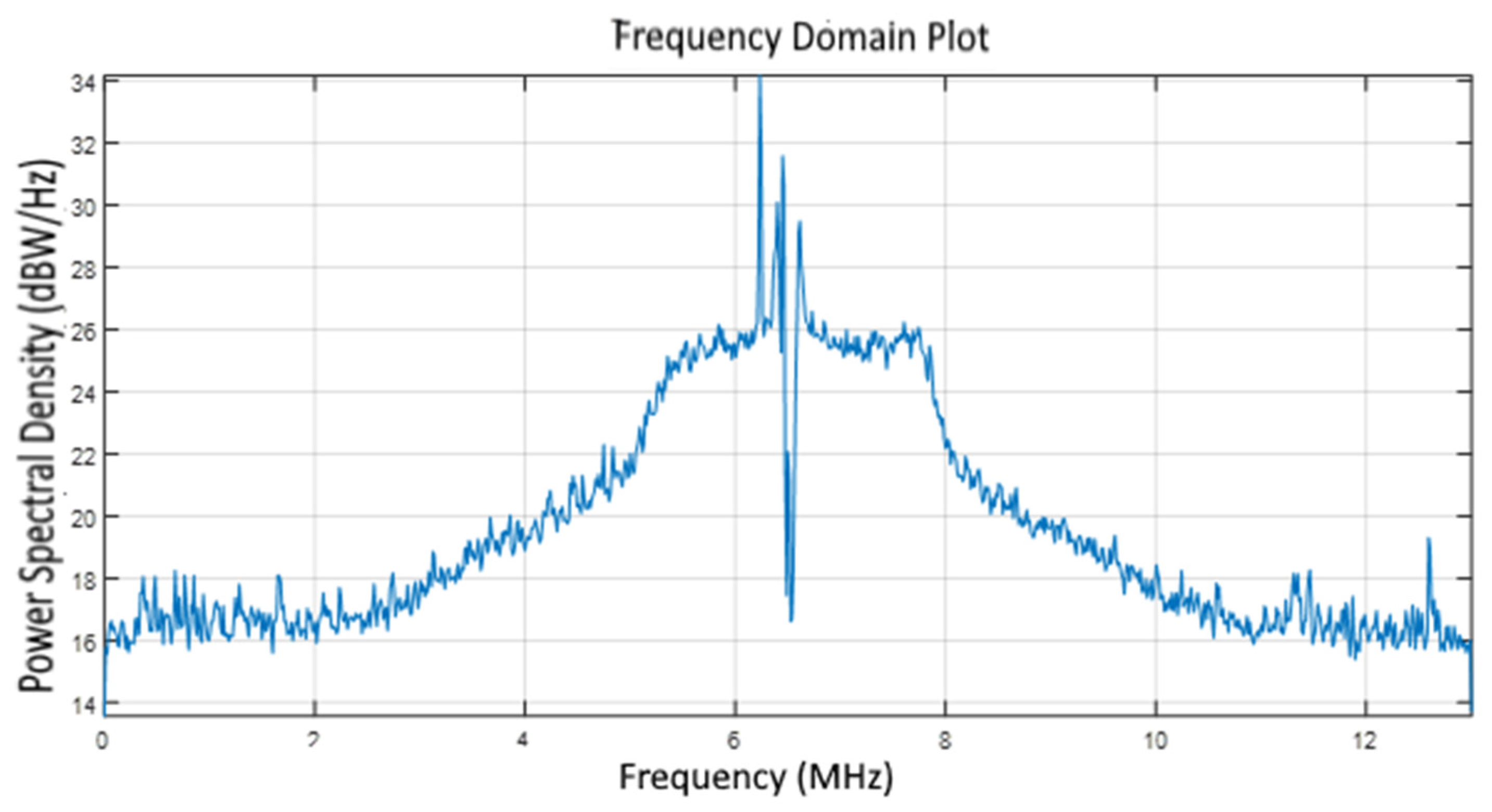
where ($fs$) is the sampling frequency. Therefore, for a given front-end bandwidth, the resolution improves with the length of FFT. From this formula, increasing the FFT size results in the frequency resolution decreasing (better resolution). As a result, the FFT results will have more points and represent the spectrum of the signal more precisely, since the distance between these bins (in terms of the frequency resolution) is smaller. If a narrowband (bandwidth less than one bin) jamming signal is not periodic within the length of FFT, its frequency spectrum will not necessarily be confined to a single bin of FFT. Instead, the discontinuities at the boundaries of the data block taken for FFT will broaden the frequency response. In Figure 7a,b, an FFT of a 6.5 MHz CW interferer and a 6.5033 MHz CW interferer, respectively, is shown when sampling at 26 MHz and $\left(J/No\right)$ equal to 110 dB-Hz. In the case of 6.5 MHz, CW repeats every four samples and hence is periodic in FFT. Its spectral energy is contained within a single FFT bin. The receiver’s front-end filter shape is shown in Figure 7a. While in Figure 7b, the 6.5033 MHz CW is not periodic, and its frequency response is much broader. One can obviously that see more bins of FFT would need to be removed in the non-periodic jammer case. Additionally, at high amplitudes, the sidelobes can raise the effective noise floor of the receiver. In practice, a jammer is seldom perfectly synchronized with the receiver’s sampling frequency and therefore a different approach must be taken.

3.4. Windowing

One way to reduce the effects of discontinuities that accrue because of FFT is the use of a technique called windowing, which is the multiplication of the original signal by a window function $w\left(t\right)$ that reaches zero at ($t=0$) and ($t=T$). Windowing functions that start at a low amplitude, increase to the middle, and finish at a low amplitude can be applied. This form of windowing reduces the amplitude of the discontinuities at the boundaries and can significantly reduce spectral leakage. There are several windowing functions such as Hamming, BlackmanHarris, Hann, rectangle windows, etc. The Hamming window was chosen because it has the best frequency resolution for cancelling the nearest side.

The benefit of using windowing is that is mitigates the effect of spectral leakage. Windows applies the weighting factor to the input signal prior to the computing of FFT. Windowing smooths the discontinuities at the block boundary and therefore lessens the effect of the spectral leakage. However, the selection of windows should be very accurate to trade-off the reduction in the background and the effectiveness of the spectral containment of the interference tone versus the reduction in SNR.

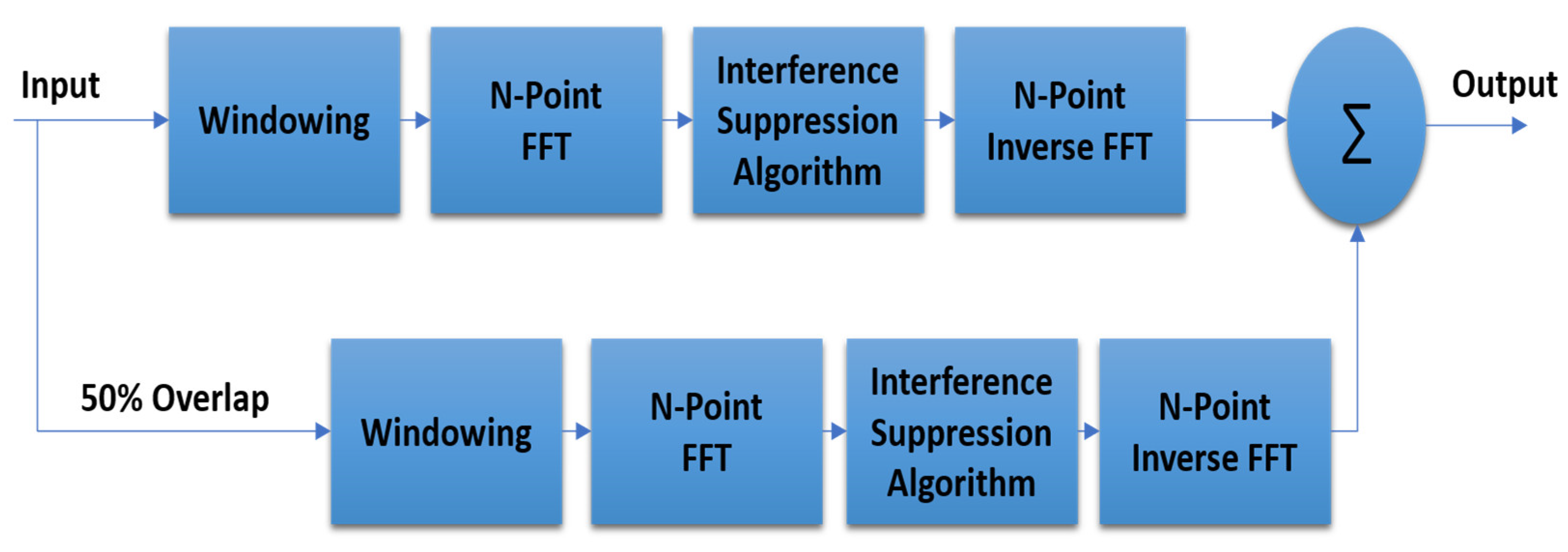
The disadvantage of windows is that by multiplying the signal by a window function, this distorts the signal, causing a broadening of the spectral peaks and worsening the resolution. The windowing inherently causes some loss in the desired signal by reducing the amplitude at the boundaries. However, this can be combated by creating two branches of the data flow with a 50% overlap (delay). The whole proposed algorithm is depicted in Figure 8. This proposed algorithm consists of 6 main stages, which are splitting the input data into two branches by a 50% overlap, applying the window, FFT, interference suppression, IFFT, and combining the two branches together [34].

In our implementation, 1024-point FFT and a 26 MHz sampling frequency were used. The 1024-point FFT was used as this is in line with the previous military ASIC devices. This results in a frequency resolution of FFT of ~25.4 kHz as calculated using Equation (3). For the GPS L1 C/A code, we considered the removal of interference in a 3 MHz passband around the centre frequency of the down-converted spectrum, so we used 119 points across our passband. It should be noted that the sampling frequency of our datalogger at 26 MHz is much greater than the frequency required for C/A code signal processing and results in more FFT points. A quarter of this rate at 6.5 MHz is a more typical sampling rate in practice and a 256-point FFT provides the same equivalent FFT resolution of ~25.4 kHz. The interference suppression is achieved by the FFT excision threshold, which is set by calculating the median value of the passband points and setting the threshold to four times its value. This threshold is roughly proportional to the mean noise power without interference and is capable of minimizing GPS signal degradation while mitigating the interference strength. Some small degradation is inevitable if the signal is always passed through the filter. Therefore, the threshold for using the filter should be set at the point the interference starts to influence the receiver. The experimental tests with CW interference confirmed that the threshold suggested in [40] is a good choice and was therefore adopted. The inherent loss of the windowing when no interference is present is effectively removed by monitoring how many bins exceed the removal threshold. If no interference passes the threshold, then the input signal is simply passed to the output to avoid loss. The signal directly passed through is delayed by a time equivalent to the FFT processing time to avoid any timing discontinuities. The next section provides an analysis of the window types.

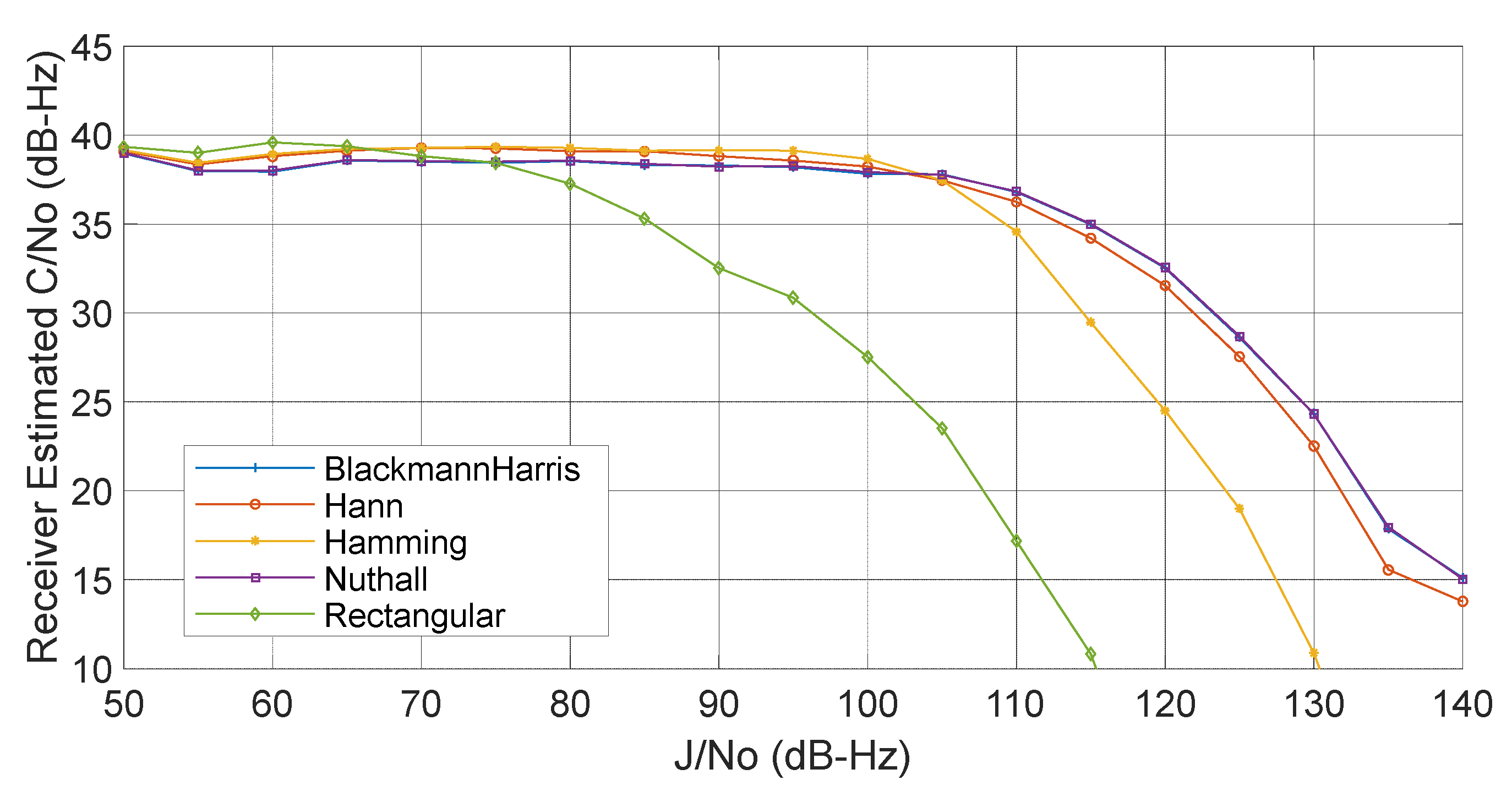
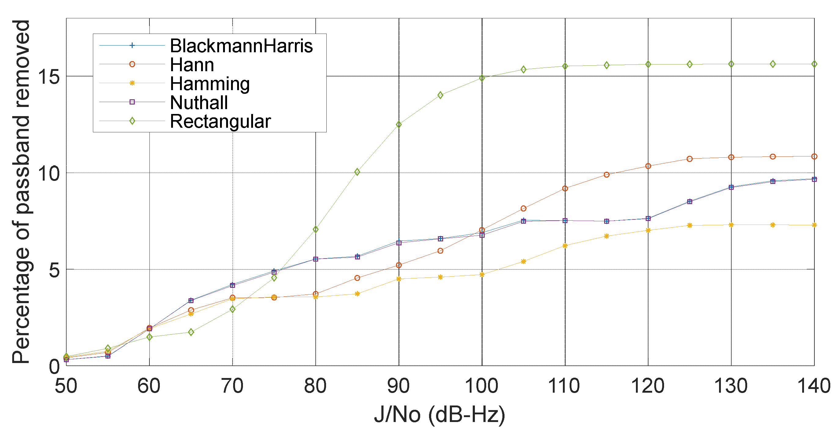
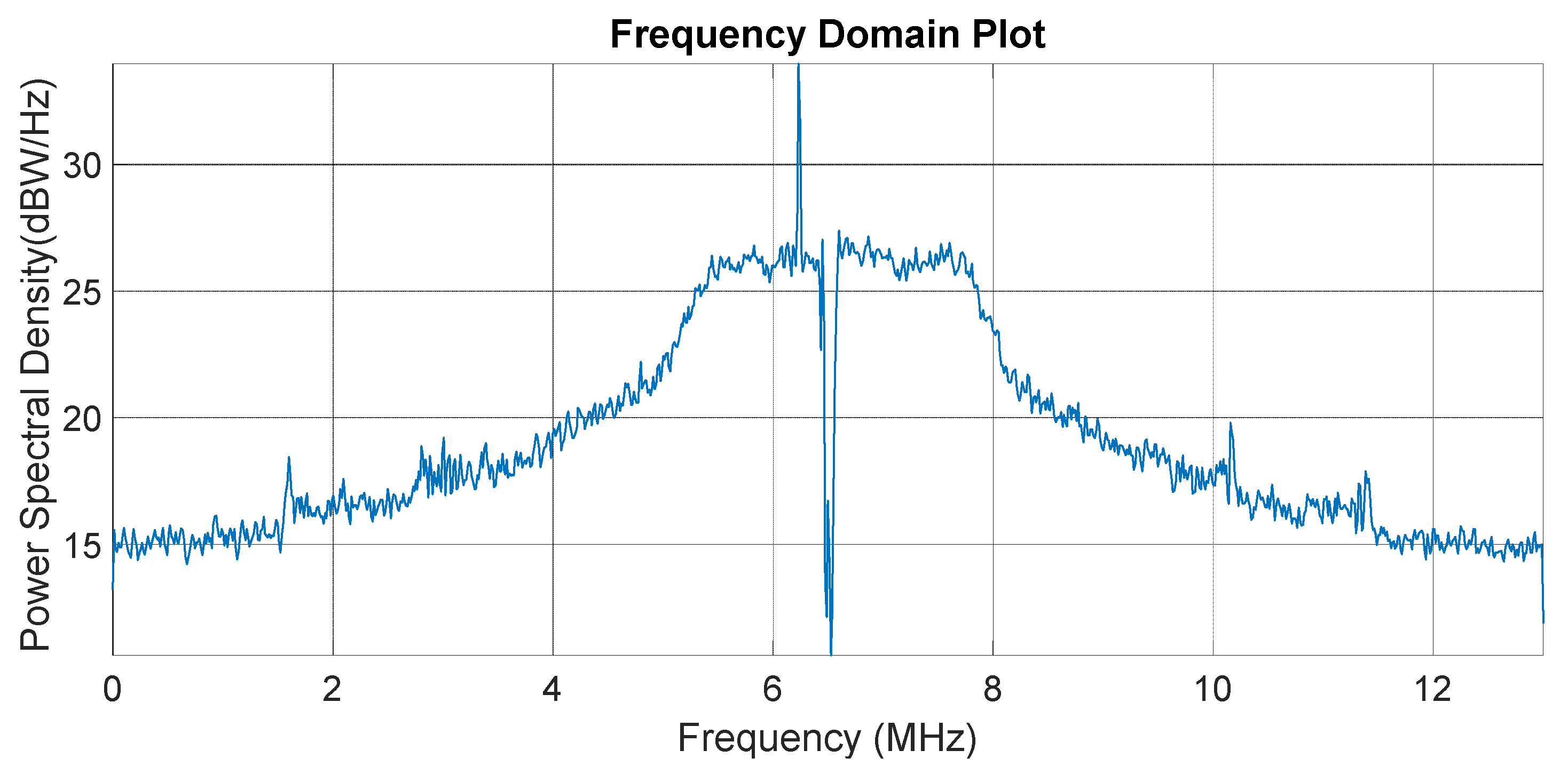
Analysis of Window Types

Figure 9 and Figure 10 show the effect of different types of windowing when a fixed frequency interference is applied to the filter depicted in Figure 8. Some windows, such as Hann and BlackmannHarris, provide a high level of interference suppression (Figure 9) while the Hamming window provides the best spectral containment (Figure 10) with reasonable suppression. The specific interference scenario determines which is the better choice. For example, the Hamming window performs well with multiple jammers as it removes less of the usable spectrum in the passband. However, if only one or two jammers are present, a BlackmannHarris window is preferable.

4. Hardware Implementation

The greatest challenge in previous studies was the hardware implementation due to the significant required number of hardware resources. FPGA was used in the implementation due to its parallelism as the hardware and software technologies are used in parallel with general reconfigurable solutions. Additionally, it has the ability to manipulate the system through software changes. FPGAs are well-structured processors that perform fast Fourier transforms (FFTs), which are often used during a GNSS receiver’s initial signal search and acquisition operations. FPGAs are generally used for prototyping GNSS receiver designs before the fabrication of a dedicated ASIC. In some cases, such as space GNSS receivers, FPGAs are used for the final product (SGR-AXIO, NAVILEO receivers).

The FPGA KCU105 kit has the Xilinx Kintex UltraScale family, which provides a hardware environment for developing and evaluating designs targeting the UltraScale XCKU040-2FFVA1156E device [41]. The Kintex UltraScale family performs ASIC-class systems with a high-level performance, clock management, and power management. This kit is suitable for prototyping for medium-to-high applications such as data centres, wireless communication, and DSP applications. 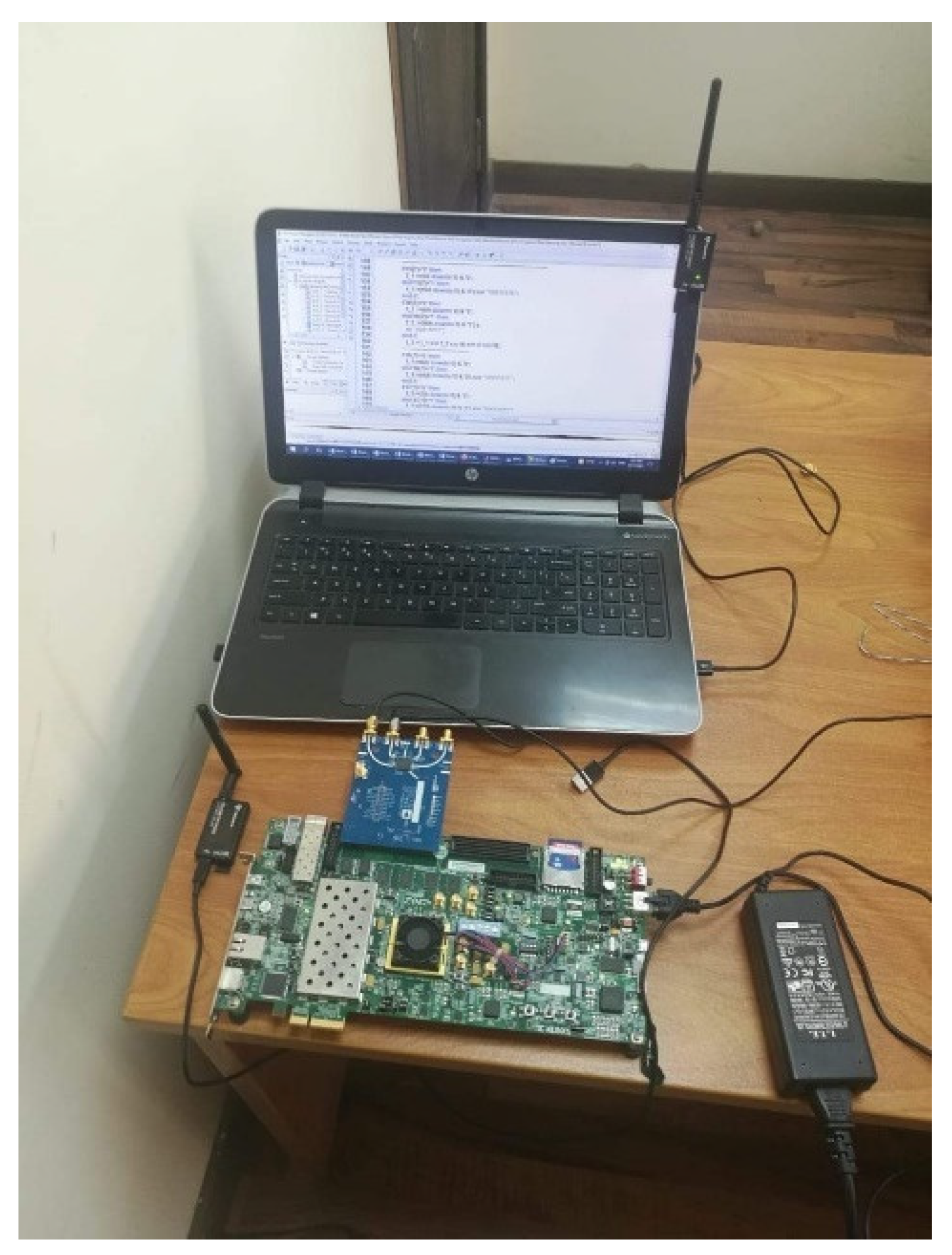This kit has a variety of features that make it suitable and sufficient for our design, such as block RAM with 21.1 MB,1920 DSP slices, and 520 I/O pins [41]. Moreover, this kit is compatible with the NAVLEO GNSS receiver. This receiver provides high-sensitivity acquisition and tracking loops. Furthermore, it supports both passive and active antennas. Additionally, it has a highly customizable and compact design, which makes it suitable for some GNSS space applications. The hardware prototype demonstration is shown in Figure 11.

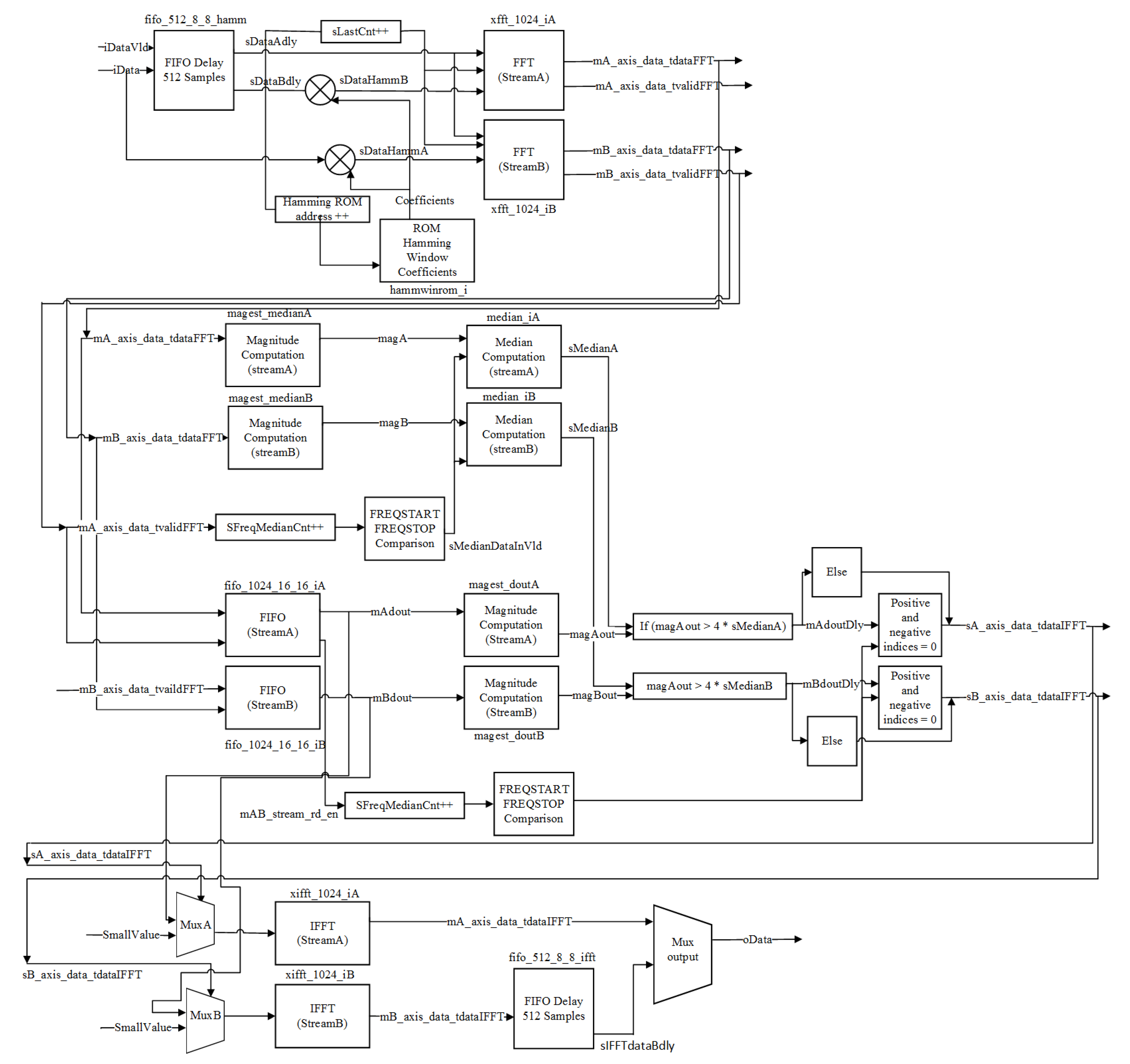
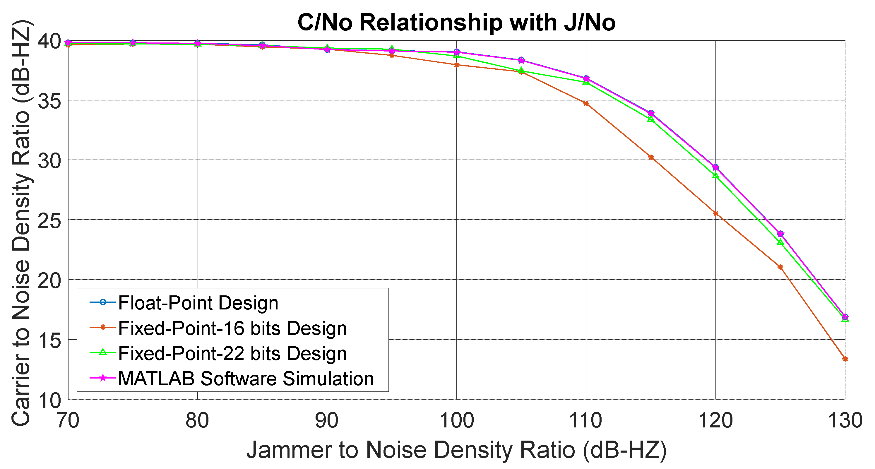
The system design was implemented with two data formats, which are fixed-point and float-point, in order to obtain the best performance design with the minimum hardware resources used. The fixed-point version was implemented by testing different precision sizes such as 8, 12, 16, 22, and 32 bits. The float-point was implemented with single-precision (32 bits). The algorithm in Figure 8 was implemented using Xilinx Vivado VHDL and each stage was validated.

Table 2. Hardware techniques and precision types.

Hardware Techniques	Precision
2 FFT 2 IFFT ROM (1 K × 8) 4 FIFO 3 Multiplexers (2 to 1)	8, 12, 16, 22, 32 bits (Fixed-Point)
2 FFT Converter (fixed to float) 2 IFFT ROM (1 K × 8) 4 FIFO 3 Multiplexers (2 to 1)	32- bit (Float-Point)

shows the hardware implementation techniques that were used based on the precision types for the hardware development stage. Figure 12 shows the block diagram of the hardware implementation for the fixed-point design. The following sections explain the processes of developing the proposed algorithm.

4.1. FFT Excision Algorithm

The FFT excision proposed algorithm is responsible for mitigating the interference from the GNSS receiver signals. This algorithm contains three inputs and two outputs. The main three inputs are the input file name, output file name, and settings. The input file contains the input file with interference, the output file contains the output without interference, and the setting contains the main GNSS receiver settings such as the time of processing, frequency sample, time of turning on the interference, and number of channels. The output of this function contains the number of frequency pins removed from branch A and the number of frequency pins removed from branch B. 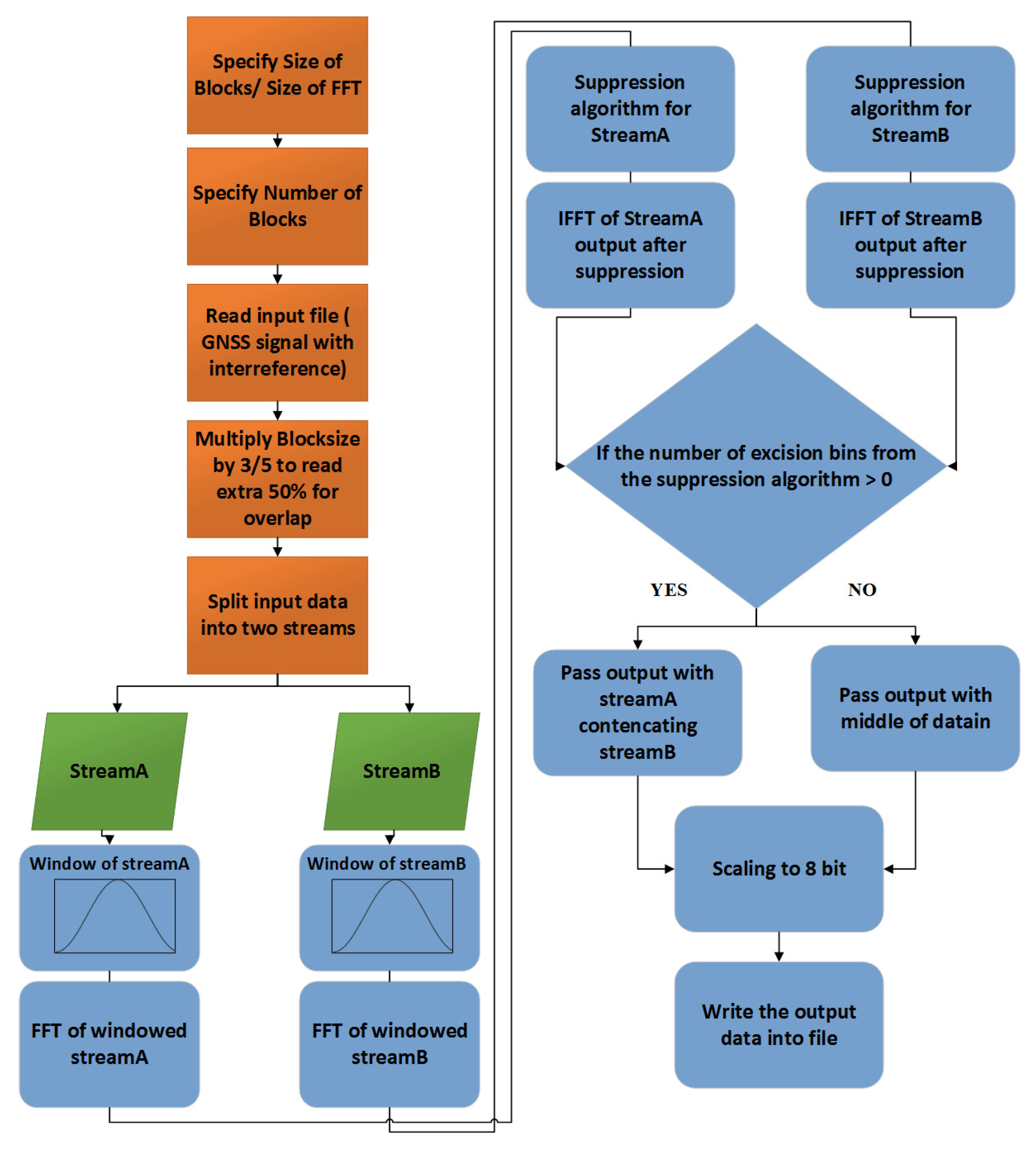Figure 13 shows the flowchart of the proposed interference excision algorithm. It illustrates how the software code works to mitigate interference in the following steps.

Firstly, the size of the block was defined based on the FFT size. In our case, the size of FFT was $2^{10}$ or 1024 points, which represents one block in the processing. Then, the number of blocks was specified based on the time of processing of the interference mitigation algorithm. For example, if the time of processing is 10,000 ms, this means the number of blocks will equal 253,906. The calculation of the number of blocks is based on Equation (4):

$$Numberofblocks=\left(mstoprocess\times \frac{fs}{blocksize}\right)-1$$

(4)

where $mstoprocess$ is the time of processing of the algorithm in ms, $fs$ is 26 MHz, and $blocksize$ is the size of FFT, which is 1024. The subtraction by one is for the 50% overlap. Then, we multiplied the $blocksize$ by 1.5 to consider the 50% overlap that occurs in the second branch as shown in Figure 8. So, the full range size is from 1 to 1536 due to the addition of an extra 512 to 1024. As mentioned previously in Section 3.4, this overlap avoids data loss and reduces the effect of the signal attenuation from the window on the output SNR. After this, based on the algorithm in Figure 8, the input data was divided into two streams. The first stream is called stream A. This stream starts from 1 to 1024 of the blocks. The second stream is called stream B. This stream is a delayed version of stream A by 50%, which starts from 512 to the end of 1536.

Next, we defined the window size, which should be the same size as FFT. As discussed previously, the Hamming window was chosen with a size of 1024. Next, the hamming windows were multiplied by stream A and stream B. After this, FFT was applied to stream A and stream B to obtain the frequency domain of both streams. After the application of FFT, the algorithm of the suppression of the interference was applied to mitigate the interference, which is explained in Section 4.2. Then, the inverse fast Fourier transform (IFFT) was applied to the output of the suppression function of stream A and stream B to go back to the time domain. Finally, if interference was found in stream A or stream B, the first half of the output (0 to 512 points) was filled by the centre of stream A (256 to 768 points) and the second half of the output (512 to 1024 points) was filled by the centre of the stream (256 to 768 points). If no interference was found, then the middle of the input data (256 to 1280 points) passed to the output.

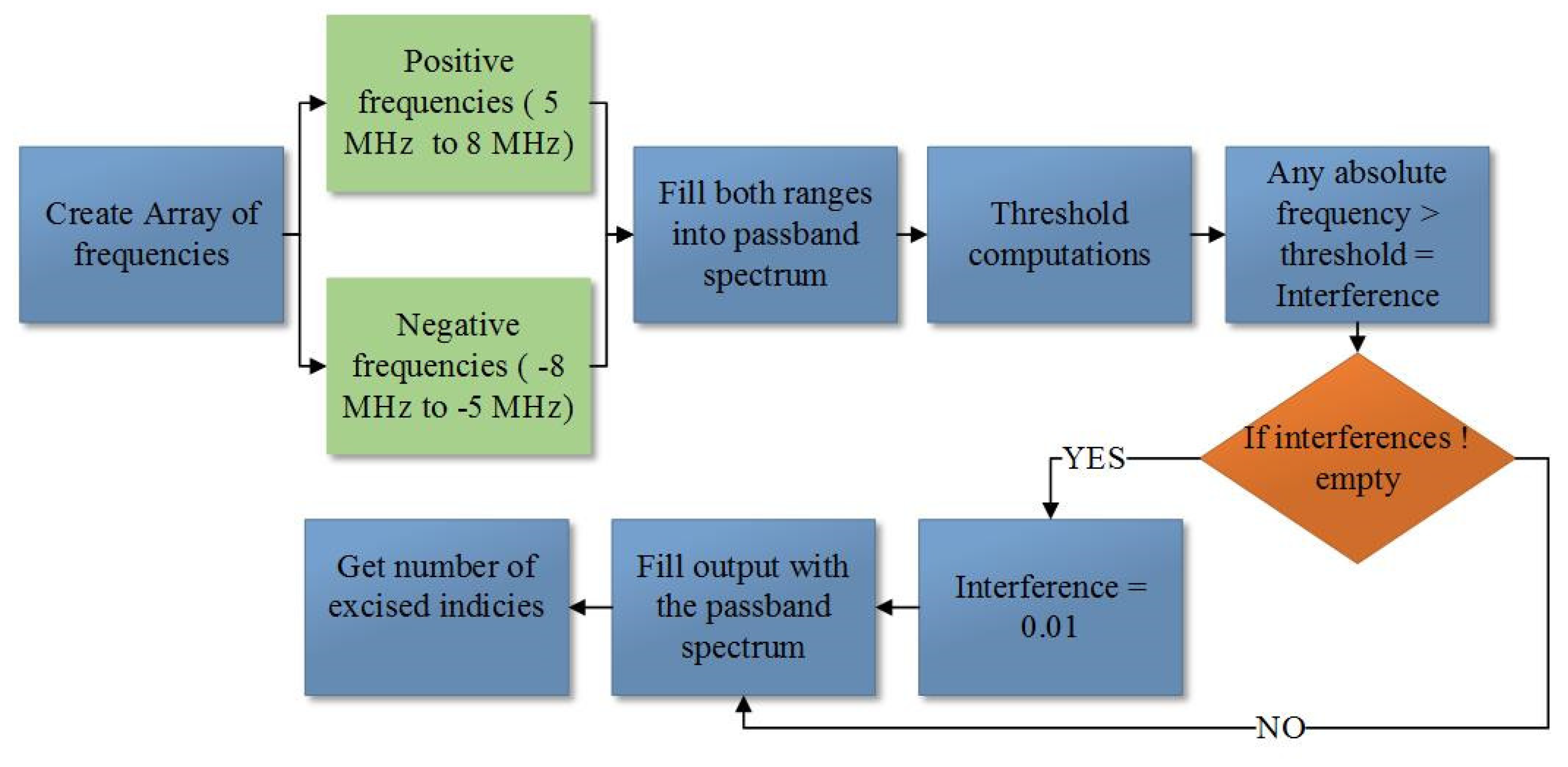
4.2. Interference Suppression Algorithm

This proposed algorithm takes the input data from the output of FFT using the same settings as the GNSS receiver and the output is the output spectrum without interference and the number of pins that were removed during the mitigation process. A flowchart of the interference suppression algorithm is shown in Figure 14. The removal method works in the range of 5 to 8 MHz according to the MAX2769 chip, which is a type of GPS receiver [42]. As mentioned in Section 3.4, the frequency resolution of FFT is ~25.4 kHz. For the GPS L1 C/A code, we considered the removal of the interference in a 3 MHz passband around the centre frequency of the down-converted spectrum. By dividing 3 MHz over the frequency resolution, we obtained the number of points across this passband, which was ~119. So, during the mitigation process, the positive and negative ranges of the frequencies were specified. The positive range ranged from 5 to 8 MHz and the negative range ranged from −8 to −5 MHz. Then, an array was created to contain the positive and negative range of frequencies. To remove the interference, a thresholding algorithm should be applied for the suppression of the interference. This threshold is one of the popular algorithms for mitigating or removing interferences. The threshold is a value where any value of the frequency exceeds a certain threshold, which will be flagged as interference to be removed.

One of the difficulties in the thresholding algorithm is the setting of the value of the thresholding. If the threshold is set too high, the interference passes without mitigation. If the threshold is set too low, the original data is removed along with the interference. Therefore, the determination of the threshold should be accurate and valid. The threshold was calculated by multiplying four of the median with the input data according to [40]. Then, the threshold was set based on the result. Based on the different testing scenarios, we found that it the removal of jamming signals once they start to influence the GNSS signals is a good choice as in [40]. After this, a comparison of all values of the frequencies with the median value is provided. Any value that exceeds the threshold is considered interference. Then, they can either be nulled or replaced by zero. Finally, the output contains the values after the removal of the interference. The number of excised bins is equal to the length of the interferences found according to the threshold. This method works relatively well and is sufficiently fast for real-time processing.

5. Results

This research aimed to compare the VHDL hardware implementation with the software-developed algorithm in MATLAB. The comparison was obtained using the input data after the addition of the interference of the MATLAB software GNSS receiver as the same input for the VHDL test bench. Then, the output of the VHDL test bench was compared with the final output from the MATLAB-developed algorithm. The stages of the hardware implementation of the FFT mitigation algorithm were written into files to be verified with each stage of the software MATLAB algorithm. For comparison and verification, the designed hardware system was validated as the optimal hardware design, and it is ready for real-time hardware implementation into KCU105 FPGA. The hardware implementation has two types of designs, which are the fixed-point design with different precision and the float-point design. Both designs were tested and verified with the MATLAB software algorithm in order to achieve the optimal design that can achieve the best performance $\left(C/No\right)$ with minimum hardware resources. The following sections discuss the simulation results and the VHDL hardware implementation validation stages.

5.1. Addition of Interferences

Before applying the interference mitigation algorithm, the interference signal should be added to the original raw data. ($J/No$) is the value of the ratio of jamming to signal and it ranges from 0 to 130 dB-Hz. The jammer frequency is calculated by $\left(f_0+d{f}_i\right)$, which is within the interval of [5.5–7.5] MHz. The interference type is 0 for the CW jammer or 1 for the sweeping jammer. The setting contains different parameters such as the frequency sampling, which is 26 MHz; the skipping number of bytes; the number of channel; the time of processing (ms), etc. Figure 15 shows the original signal in blue with the added interference signal in red, with ($J/No$) equal to 80 dB-Hz. It is obvious that the interference covers the whole original signal. The same type of jammer in Figure 15, which is CW shown in Figure 16, but with 4 CW jammers was added with different jammer frequencies of 5.5, 6.5, 6.5033, and 7 MHz, with ($J/No$) of 40 dB-Hz.

The original signal with the added jammers is shown in Figure 16. It is noticeable that when we increase the ($J/No$) value, the interference shape becomes sharper, which means the distortion of the original signal increases as well. Figure 17 shows the original signal in blue with the added sweeping jammer signal in red. Markedly, the sweeping interference is stronger than the continuous wave (CW) because it uses a range of frequencies to attenuate the signal while CW uses a fixed frequency.

Other different scenarios were tested by changing the value of the jammer frequency to ensure it is within [5.5 to 7.5 MHz]. For each scenario, a different value of jamming-to-noise ($J/No$) was tested to validate the value of the carrier-to-noise $\left(C/No\right)$ in dB-Hz. Figure 18 displays the $\left(C/No\right)$ degradation with different types of jammers. The blue line represents a single CW jammer, and the red line represents five CW jammers. The green line represents a sweeping jammer. It shows that the sweeping jammer results have the worst $\left(C/No\right)$ compared to the CW single jammer and the five CW jammers. After applying the mitigation filter in Figure 19, the performance of $\left(C/No\right)$ increased. With a ($J/No$) value of more than 70 dB-Hz until 90 dB-Hz, the single jammer and multi-CW jammer lines dropped rapidly to reach $\left(C/No\right)$ of below 25 dB-Hz. The sweeping jammer signal reached less than 20 dB-Hz when the ($J/No$) value was 90 dB-Hz.

5.2. Xilinx FFT Model

The challenge in hardware implementation is the significant time needed to obtain the final sampled output signal after the removal of interference. Simulation testing depends on the collected input data from the GNSS receiver. To overcome this challenge, the Xilinx FFT model was developed to be part of the testing and validation. This model was developed according to [43]. The Xilinx FFT model contains the FFT MEX function, which provides the MATLAB software interface to the FFT Xilinx model. This function produces identical results to the Xilinx FFT IP core. This model is useful as it has a lot of variable parameters to be changed as required. Three of these important parameters are the formatting type, scaling option, and input width. By testing this model with different precision for fixed-point formatting, the Xilinx FFT model results state that increased precision provides a better performance signal.

Significantly, there are matching differences in the precision between the fixed-point 8-bit Xilinx FFT model points and FFT MATLAB-based points. This is because the FFT MATLAB-based point uses the 64 double-precision float-point while the 8-bit precision fixed-point is used for the Xilinx FFT model. The percentage error of the fixed point 8-bit precision Xilinx FFT model and the FFT MATLAB-based point is 9.5622%. The points of the fixed-point 16-bit precision Xilinx FFT model and FFT MATLAB-based point match better than the 8-bit precision and the percentage error is 2.3677%. The points of the fixed-point 22-bit precision Xilinx FFT model and FFT MATLAB-based point are almost identically matched and the percentage error is 0.0074%. The points of the float-point with the single precision of the Xilinx FFT model and FFT MATLAB-based point are the closet matched results due to the similarity of the data format, which is the float-point, and the percentage error is 0.0013%.

5.3. Validation Results and Discussion

Verification of the results of the VHDL implementation was achieved by comparison with the MATLAB software algorithm. The validation results were the Hamming window validation, FFT validation, excised data validation, IFFT validation, and the final output validation. The fixed-point and float-point designs were tested and verified. The output results were tested with different levels of ($J/No$) and different jamming frequencies for two types of interference, which are CW and the sweeping jammers. In order to achieve the best results of the mitigation algorithm, a high level ($J/No$) was chosen of 80 dB-Hz with a frequency jammer equal to 6.5033 MHz for both CW and the sweeping jammer as the test input file. Figure 20 shows the input sampled signal with the CW jammer at $\left(J/No\right)$= 80 dB-Hz and freqj = 6.5033 MHz. Figure 21 shows the output sample signal in the frequency domain after the application of the MATLAB FFT excision.

In the fixed-point design, we noticed that when we increased the precision of the fixed-point design, the performance of $\left(C/No\right)$ improved. In other words, an increase in the precision improved the performance but consumed more hardware resources. The fixed-point design with 8-bit precision showed the worst performance due to the low precision. Figure 22 shows the final frequency spectrum from the 8-bit precision fixed-point design. It is obvious that the shape of the spectrum is significantly unmatched with the output signal from the MATLAB FFT excision algorithm in Figure 21. The 32-bit precision, 22-bit precision, and 16-bit precision fixed-point designs showed the most matched results with the MATLAB software algorithm. Figure 23 shows the final output of the frequency domain of the fixed-point design with 16-bit precision. The frequency spectrum of the fixed-point design with 16 bits in Figure 23 shows similar results to the frequency spectrum of the MATLAB software simulation in Figure 21. However, the attenuation results of the final output do not perfectly match the MATLAB result. The existence of interference with the output from the start of the frequency axis is noted and this is due to FFT output. The FFT results of stream A indicate a low-frequency point of FFT. Generally, low-frequency noise could be additionally filtered, which produces little noise that affects the final output. Moreover, the precision of the fixed-point (16-bit) of Xilinx-FFT is different than the float-point double-precision of FFT-MATLAB. For this reason, the fixed-point design with 22-bit precision was chosen as the best optimal design according to the fixed-point design. The final frequency spectrum for the 22-bit precision fixed-point design is shown in Figure 24.

For these reasons, the float-point design was developed to achieve a better performance than the fixed-point performance due to its float-point double precision. The float point design showed the best results, which matched the MATLAB algorithm results, compared to the fixed-point design. Figure 25 shows the sampled signal from the VHDL implementation in the frequency domain. It is obvious that the shape of the VHDL output signal is very similar to the sampled signal from the MATLAB software algorithm in Figure 21. There is a small difference in the attenuation of the interference due to two reasons. The first reason is the precision difference as the FFT MATLAB-based point uses a double-precision float-point (64-bit) while in the VHDL hardware implementation, the FFT IP core uses a single-precision float-point (32-bit). The second reason is the magnitude calculation for the threshold computation as the estimated calculation is used in the hardware implementation while a real calculation is used in MATLAB, which achieved full precision. However, this difference between the MATLAB results and VHDL results does not affect the performance of the desired navigation and tracking loops as the Xilinx FFT model results were tested to obtain the value of $\left(C/No\right)$. The mean was $~$40 dB, which is sufficient for GNSS receiver operations. The float-point design gives the most matched results with the MATLAB simulation software with the largest amount of hardware resources.

Figure 26 shows the relationship between the fixed-point design with 16-bit precision, fixed-point design with 22-bit precision, and float-point design using the Xilinx FFT model and MATLAB software simulation. It illustrates that the float-point design has a better performance than the fixed-point design according to $\left(C/No\right)$. Additionally, the float-point design using the Xilinx FFT model has a similar performance to the MATLAB simulation. The blue line of the float-point design starts to fall when $\left(J/No\right)$ is equal to 70 dB-Hz to reach 39 dB-Hz of $\left(C/No\right).$ In contrast, the fixed-point design with 16-bits sharply decreases to less than 35 dB-Hz of $\left(C/No\right)$ once $\left(J/No\right)$ reaches 80 dB-Hz. The fixed-point design with 22-bits shows a better performance than the fixed-point design with 16-bits. The fixed-point with 22-bits has a $\left(C/No\right)$ value equal to 28 dB-Hz when $\left(J/No\right)$ reaches 90 dB-Hz. The fixed-point with 16-bits reaches a $\left(C/No\right)$ value equal to 26 dB-Hz when the $\left(J/No\right)$ value is equal to 90 dB-HZ.

The float-point design consumes more hardware resources than the fixed-point design due to the nature of the float-point length and mathematical operations. The performance of the filtered algorithm drops dramatically below the fixed-point design with 16-bits while the fixed-point design with 22-bits shows a better performance compared to other precisions of FFT. Therefore, the fixed-point with 22-bits design was chosen as a compromised solution as it achieved the desired performance using the required hardware resources compared to the float-point design. This standard of performance is significant for GNSS receiver operations such as acquisition, tracking, and navigation. These operations require a reliable, accurate, and robust performance due to their critical jobs. For this reason, the fixed-point design with 22-bits was chosen as the optimal solution for hardware implementation, trading off the desired performance against the required hardware resources. A complete $\left(C/No\right)$ comparison is shown in

Table 3. Comparison of the $\left(C/No\right)$ values of the 16, 22-bit (fixed-point), 23-bit (float-point), and MATLAB software simulation performances.

Jamming Power (dB)	$\mathit{C}/\mathit{N}\mathit{o}$ Values (dB/Hz)
	Fixed-Point (16-bit)	Fixed-Point (22-bit)	Float-Point (32-bit)	MATLAB Software Simulation
70	39.5972	39.6920	39.7801	39.7800
75	39.6817	39.6863	39.7672	39.7672
80	39.6437	39.6462	39.7286	39.7285
85	39.4238	39.5411	39.5991	39.5291
90	39.2320	39.3361	39.2081	39.2081
95	38.7204	39.2509	39.1114	39.1003
100	37.9354	38.6885	39.0239	38.9853
105	37.3484	37.4288	38.3245	38.2986
110	34.7053	36.4707	36.8067	36.7809
115	30.2256	33.3656	33.9007	33.8564
120	25.5357	28.6583	29.3876	29.3586
125	21.0347	23.0821	23.8284	23.8035
130	13.3749	16.6888	16.8952	16.8751

. The $\left(C/No\right)$ comparison confirms that the fixed-point 22-bit showed the best performance compared to the fixed-point 16-bit. Moreover, the hardware implementation using the fixed-point 22-bit showed a similar result to the MATLAB software simulation. A comparison of the utilization percentage of the hardware design resources between the fixed-point design (22-bit) and the float-point design (32-bit) is shown in

Table 4. Hardware design resources of the fixed-point (22-bit) and float-point (32-bit) design.

Hardware Design Resources	Fixed-Point (22-bit) Utilization	Float-Point (32-bit) Utilization
CLB LUTs	1599	2871
LUT as logic	1343	2015
LUT as memory	256	977
CLB Registers	1046	6821
Registers as Flip flop	1045	6820
Registers as Latch	1	1
Block RAM	2.5	19
36 Kbits RAM block	0	0
18 Kbits RAM block	5	38
URAM	0	0
DSPs	40	66

. The comparison clearly shows that the float-point design consumed more hardware resources than the fixed-point design.

5.4. Hardware Implementation Challenges and Comparison with Related Work

One of the main challenges of the VHDL implementation is the magnitude calculation in the proposed algorithm. It is easy to perform DSP calculations in MATLAB. However, performing magnitude calculations in the hardware implementation is challenging. Efficient calculation of the square root operation was accomplished in the VHDL implementation using an optimization technique to accomplish high-speed magnitude approximation. The algorithm that is used to compute the magnitude of a complex vector of the FFT results (real and imaginary parts) is improved as “alpha max plus beta min”. In addition, the median calculation is another challenge in the VHDL implementation. The median calculation is required for the threshold of the FFT excision filter algorithms. The calculation of the median is optimized using a histogram visualization technique. The histogram represents the number of FFT bins, and each bin has a value.

The main optimization of the hardware implementation is the analysis of the required precision for the fixed-point implementation to provide a more efficient design than the floating-point FFT. The usage of hardware resources was reduced to 44.3% using the fixed-point design. This is a very time-consuming analysis as it requires the GNSS software receiver to be run multiple times on the output of the FFT simulation for each bit depth. Another FPGA-specific issue is how data is passed through when no interference is present, so the output is continuous regardless of whether the removal is performed as explained in Section 4.1.

The algorithm in [44] works well against pulsed noise interference but not with CW or narrowband interference such as our proposed technique. Their findings demonstrated that the HDDM methods cannot successfully mitigate the CW interference since the minimal frequency resolution corresponds to one FFT bin and is in the range of 2–3 MHz. Their results showed a small improvement over the mass market receiver toward the CW and narrow sweeping jammers, as with the high power of interference, there is high degradation of $\left(C/No\right)$, which can reach <20 dBHz. On the other hand, the proposed hardware implementation of the FFT excision filtering algorithm works with high-power CW interference while maintaining the desired $\left(C/No\right)\cong 40\mathrm{dB}$. The proposed HDDM uses multiple frequency bands with different windowing functions; hence, this results in the use of more hardware resources. This appears to be reflected in their resource allocation, using 13,625 LUTs compared to 1600 in our 22-bits (fixed-point) design and 159 DSPs compared to 40 in our proposed design.

6. Conclusions

This paper emphasized FFT excision as an interference mitigation technique that can provide significant improvements in current receiver performance. This proposed approach can deal with different levels of $\left(J/No\right)$ and two types of narrowband interference, which are the continues-wave (CW) jammer and sweeping jammer. Previous researchers showed a significant impact of this approach in terms of software development while none of them implemented this algorithm due to the complexity and the significant hardware resources required for hardware implementation. The aim of this work was to show that the use of fixed-point implementation in a current FPGA can now be efficiently realized and utilized. This makes the proposed approach using 1024 points of FFT feasible and doable for obtaining the desired performance with the required hardware resources. The results show that this approach is powerful and can deal with different levels of interference while maintaining the desired $\left(\left(C/No\right)\cong 40\mathrm{dB}\right)$. The algorithm was implemented using VHDL to be uploaded into FPGA for hardware implementation. The hardware implementation has two designs, which are fixed-design and float-point. Each design was validated and compared with the MATLAB-developed algorithm. The float-point design showed the best performance using a larger number of hardware resources compared to the fixed-point design. However, the fixed-point with 22-bits design provided a performance that is very close to that of the float-point design performance with fewer hardware resources. Therefore, the fixed-point with a 22-bits FFT excision algorithm was chosen as the optimal design and compromised solution.