1. Introduction
Hysteresis phenomena are prevalent in various technological domains, resulting in a growing interest in models of the magnetization processes. Jiles and Atherton [
1] proposed a model for describing the magnetization of soft magnetic materials. From an engineering point of view, this model is attractive because of the physical interpretation of the parameters that define it and the fact that it is based on the physical insight of hysteresis. However, as noted in [
2], the iterative procedure of estimating model parameters poses convergence problems. The model is also extremely sensitive to initial parameter values and hence requires physical experimentation on the material to identify the starting point. Therefore, researchers have tried a host of different techniques to reduce the sum of squared errors (SSE) between experimental and modelled hysteresis curves. Some of these attempts include implementations of global optimization techniques, for example, simulated annealing methods [
3], metaheuristic techniques such as genetic algorithms [
4,
5], machine learning techniques such as neural networks [
6], or an exhaustive search in the solution space [
7].
Section 2 shows that Jiles–Atherton model parameters are clearly connected with the physical properties of magnetic materials. However, there is no definitive method to calculate the value of each Jiles–Atherton model parameter. All of the methods use optimization algorithms to minimize the objective function, which is defined as the sum of squares of differences between the experimental hysteresis curve and the hysteresis curve as a result of modeling. Unfortunately, this sum exhibits many local minima, and hence gradient optimization techniques strongly depend on the starting point.
The traditional method of estimating model parameters [
1] assumed knowledge of measured slopes
dH/
dM on several characteristic points on the hysteresis curve. This information facilitated the development of a set of nonlinear equations, which were solved iteratively to obtain the values of model parameters using numerical Runge–Kutta-algorithm-based methods. The anhysteric magnetization equation for anisotropic materials has been solved with the Gauss–Konrod method. Optimization methods have been explored by fitting Jiles–Atherton hysteresis curves to measurement data by using techniques including nonlinear least-squares, simulated annealing [
3], genetic algorithms (binary and real-coded) [
4,
5], levy whale optimization [
8], particle swarm optimization [
9], cuckoo search [
10,
11], the covariance matrix adaptation evolution strategy, and other differential evolution algorithms [
12]. Trapanese [
6] trained a neural network with the hysteresis data and corresponding Jiles–Atherton model parameters of several materials. The trained network was used to predict the unknown Jiles–Atherton model parameters for a test material.
As optimization algorithms are time-consuming, a trial-and-error approach to Jiles–Atherton model parameter determination has also been suggested. The original paper [
1] provided plots of different Jiles–Atherton model parameters held constant while one of them was varied for isotropic materials, whereas Prigozy [
13] provided plots for anisotropic materials.
This paper aims to reduce the solution space of the Jiles–Atherton model parameters to a smaller and more manageable set using space-filling designs. In essence, we are reducing the area of the solution space that these algorithms explore, thereby cutting down drastically on the solution space and the time required to reach an optimal solution. The solution space exploration is done efficiently with a space-filling design that is described in the following sections. Once a reduced solution space is obtained, any of the aforementioned algorithms can be used to exploit and further explore the reduced solution space in order to arrive at the optimal solution. However, we focus on the genetic algorithm because it is the most robust among the algorithms [
14].
The remainder of the paper is organized as follows.
Section 2 describes the Jiles–Atherton model in detail.
Section 3 describes space-filling designs and its application to the Jiles–Atherton Model, and
Section 4 describes the genetic algorithm for identifying the parameters of the Jiles Atherton Model. The conclusions follow in
Section 5.
2. Jiles–Atherton Model
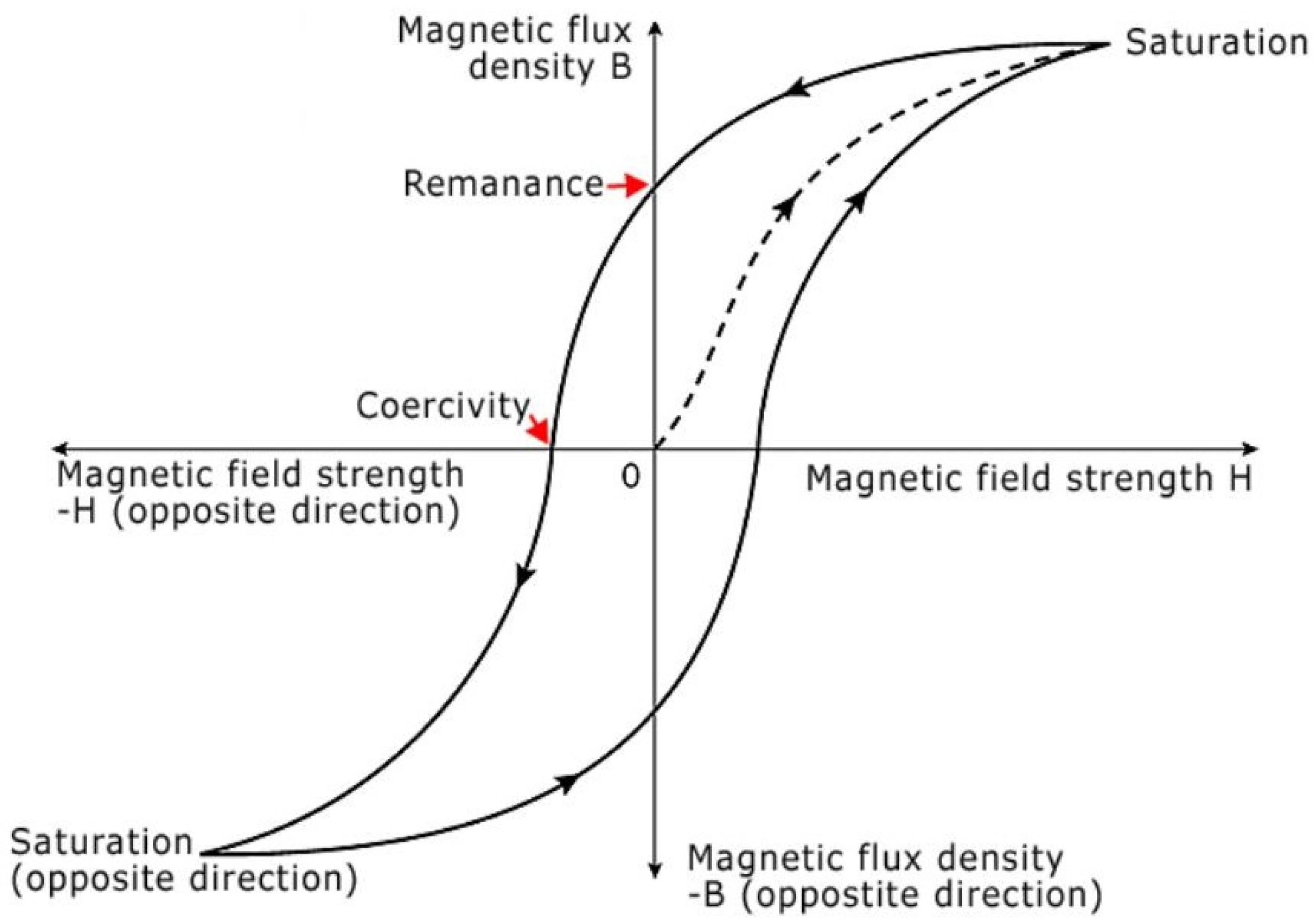
The Jiles–Atherton [
1] accounts for all important features of the hysteresis curve (
Figure 1)—initial magnetization curve, saturation of magnetization, coercivity, remanence/retentivity. The Jiles–Atheron model was developed for anhysteric magnetization (
Man) using the mean field approach [
1]. The effects of magnetic domain wall pinning on defect sites are then considered to account for hysteresis. Examples of defect sites include grain inhomogeneity, for example, angles of dislocation, inhomogeneous strain regions, etc.
The following expression represents the effective magnetic field,
where
α is a parameter representing the experimentally determined inter-domain coupling, and
H is the magnetizing field. For an isotropic material, the magnetization response to this effective field is expressed as
where
MS is the saturation magnetization of the ferromagnetic material with unit A/m, and
f is a function to be defined. This magnetization expression accounts for the magnetic field response and the mean magnetic interaction with the rest of the material using the term
αM, and hence is only a statistical domain distribution. Hence, it does not account for pinning and is considered the anhysteric magnetization. The modified Langevin equation is considered for
f, which leads to the following expression for anhysteric magnetization,
Here,
A is the anhysteric behavior parameter which characterizes the shape of the anhysteric magnetization. When the work done by the field equals the magnetization energy of the sample, the domain wall displacement stops. On removal of the field, the domain wall returns to its original location. The domain wall translation causes an energy loss called the irreversible magnetization component
Mirr, and is given by
Here,
K is the average energy to break the pinning location,
μ is the initial permeability of the material, and
The total magnetization is given by
Here, C is the magnetization reversibility proportion.
Various modifications/additions were made to the Jiles–Atherton model by multiple researchers, for example:
- (a)
The original Jiles–Atherton model only considered isotropic materials. The anhysteric magnetization for anistropic materials is given by
where
E (
i) is given by
where
ϕ is the angle between the applied field and easy magnetization axis,
θ is the angle between the atomic magnetic moment and magnetizing field direction, and
Kan is the magnetic anisotropy energy density with units J/m
3. In some materials such as constructional steels, isotropic and anisotropic phases can be mixed. In these cases, the total anhysteric magnetization is calculated as per Equation (9), where
t is between 0 and 1.
- (b)
Rotating electrical machines experience rotational fluxes, which are more complicated as compared to pulsating fluxes. For the same flux amplitude, magnetic losses due to rotating fluxes are almost 3 to 5 times that of pulsating fluxes. This necessitates a vector hysteresis like the vector Jiles–Atherton model, which retains the simplicity of the original model, which is scalar, but requires the original number of parameters in each spatial direction considered [
9].
- (c)
In some scenarios, the induction is known before the field is applied. A classic example is a finite element model, where the vector Jiles–Atherton model is employed. For these simulations, an inverse Jiles–Atherton model presenting the magnetic induction as an independent variable [
10] is used, with the main equation of this model as
3. Space-Filling Design
In deterministic modeling problems such as circuit SPICE simulations, the variability is negligible, so the traditional design of experiment features such as replication, randomization, and blocking to reduce experimental variability are unnecessary. Computer deterministic models are complex and can involve hundreds of variables with interactions. Space-filling designs are used to find a simpler model form of the complex computer model called a surrogate model. Space-filling designs find accurate representations of complex computer models by spreading out the design points as far apart from each other as possible while staying within the model parameter boundaries. As opposed to traditional designed experiments that have fixed levels for each factor for each simulation, space-filling designs explore the design space between two levels more thoroughly by having different levels in every simulation. This leads to a higher coverage of the parametric space, which is extremely important in the case of the Jiles–Atherton model, which has multiple local minima.
Latin hypercube designs [
15] spread out the points in the design space more evenly across all possible values as compared to sphere packing designs. The parametric space is partitioned into intervals, and a sample is selected from each interval. Uniform design [
16] minimizes the discrepancy between the design points (which have an empirical distribution that approximates uniformity) and a theoretical uniform distribution.
The Latin hypercube was used to set up a space-filling design that explores the design space of the four Jiles–Atherton parameters
MS,
A,
C, and
K because of its computational efficiency compared to the other types of space-filling designs. By default, the number of simulations that need to be run is 10 times the number of factors, which, in this case, means 40 simulations need to be run. First, a linear model (11) is fit where the response SCORE represents the sum of squared errors (SSE) between the actual transformer’s secondary voltage and the transformer’s secondary voltage simulated on PSpice. The analysis is carried out using SAS JMP software.
The estimates of the regression coefficients of the linear model (11) are given in the ‘Estimate’ column in
Table 1, whereas the column ‘Std Error’ gives the standard deviation of each of the parameters. The ‘t Ratio’ column gives the t ratio metric, which tests whether the true value of the parameter is zero. It is a ratio of the estimate to its standard error, and under the null hypothesis (true value of parameter is zero), has a Student’s t distribution. The ‘Prob > |t|’ column lists the
p-value for the test where the true parameter value is zero. A
p value of less than 0.05 implies that the parameter is statistically significant at the 95% confidence level. The goodness of fit of the linear model (11), as measured by the metric RSquare Adjusted, which is the coefficient of determination adjusted to account for overfitting, is 0.71 or 71%. As can be seen from
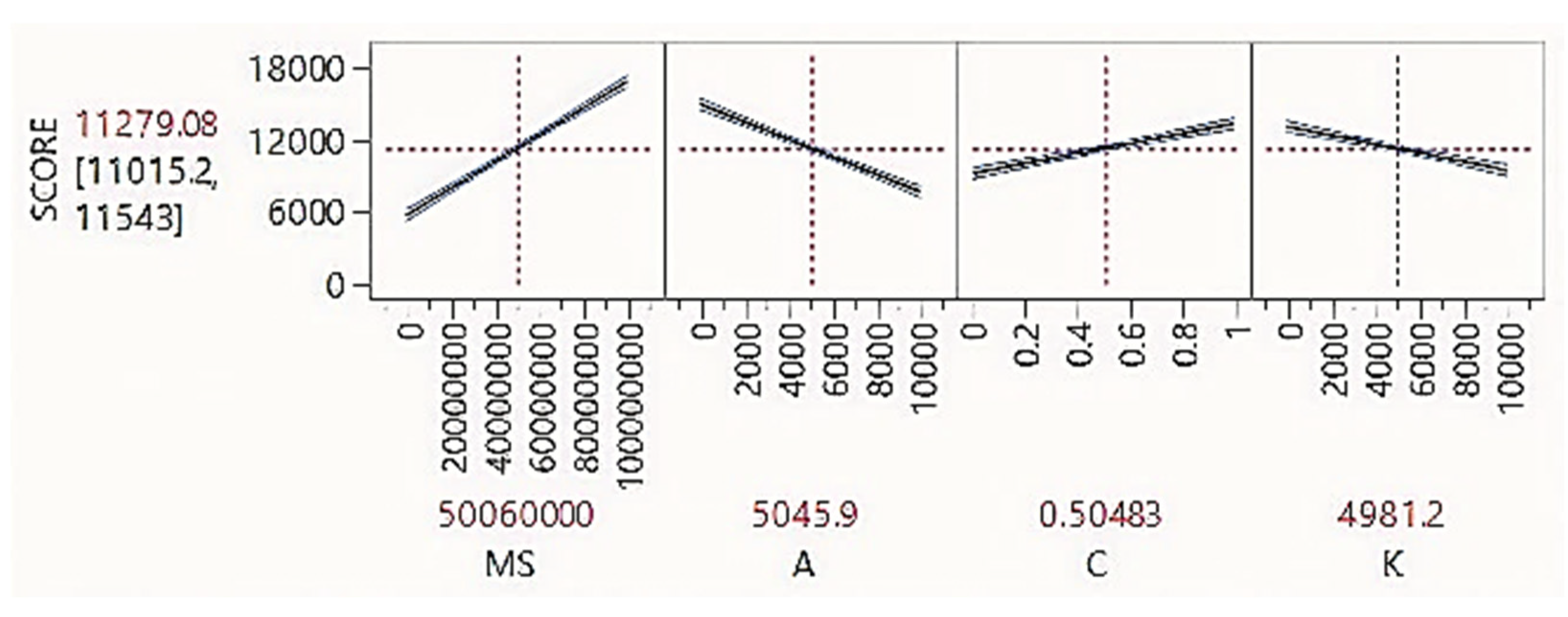
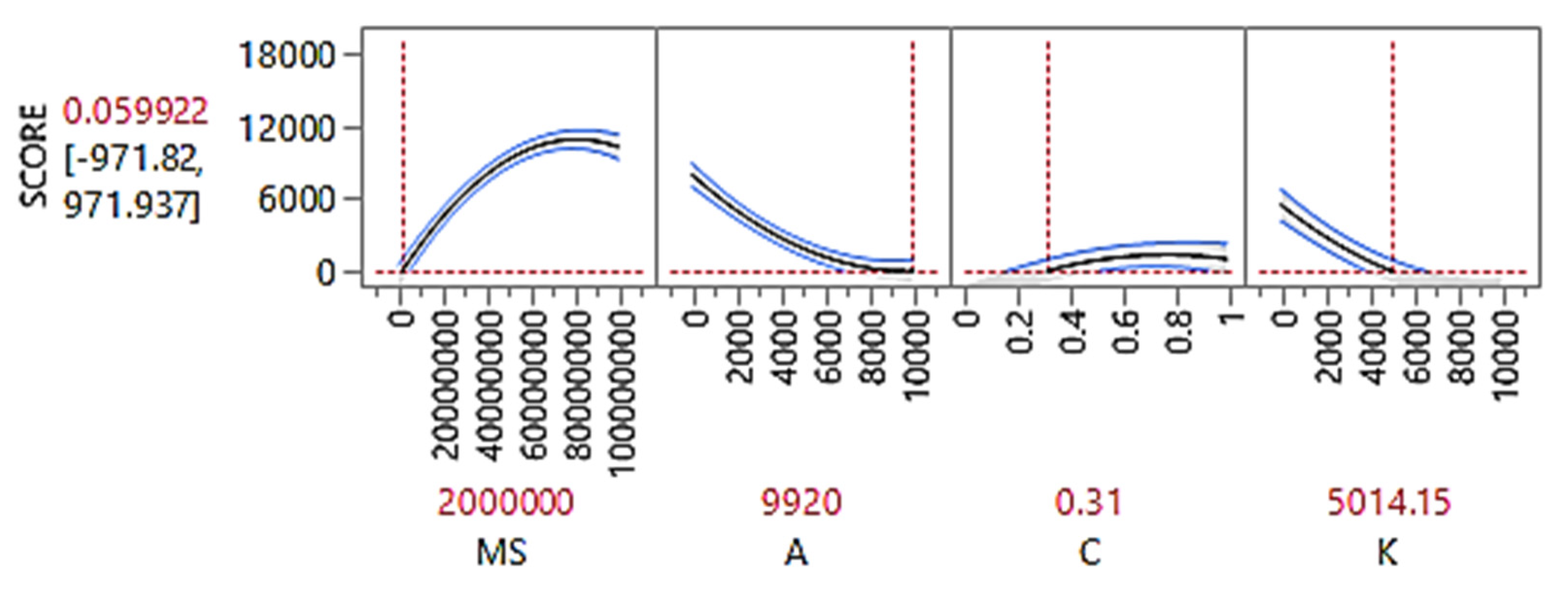
Table 2, as expected, all Jiles–Atherton model parameters are statistically significant to the SCORE at the 95% confidence level. JMP has the option of a prediction profiler (
Figure 2) that can be used to vary the parameter values simultaneously to bring the SCORE (SSE) to zero (
Figure 3).
Figure 2 and
Figure 3 show the individual response surfaces of the different Jiles–Atherton model parameters. The slopes of the response surfaces are the values in the ‘Estimate’ column of
Table 1, which in turn are the regression coefficients of the linear model (11). The larger the absolute value in the ‘Estimate column’ of
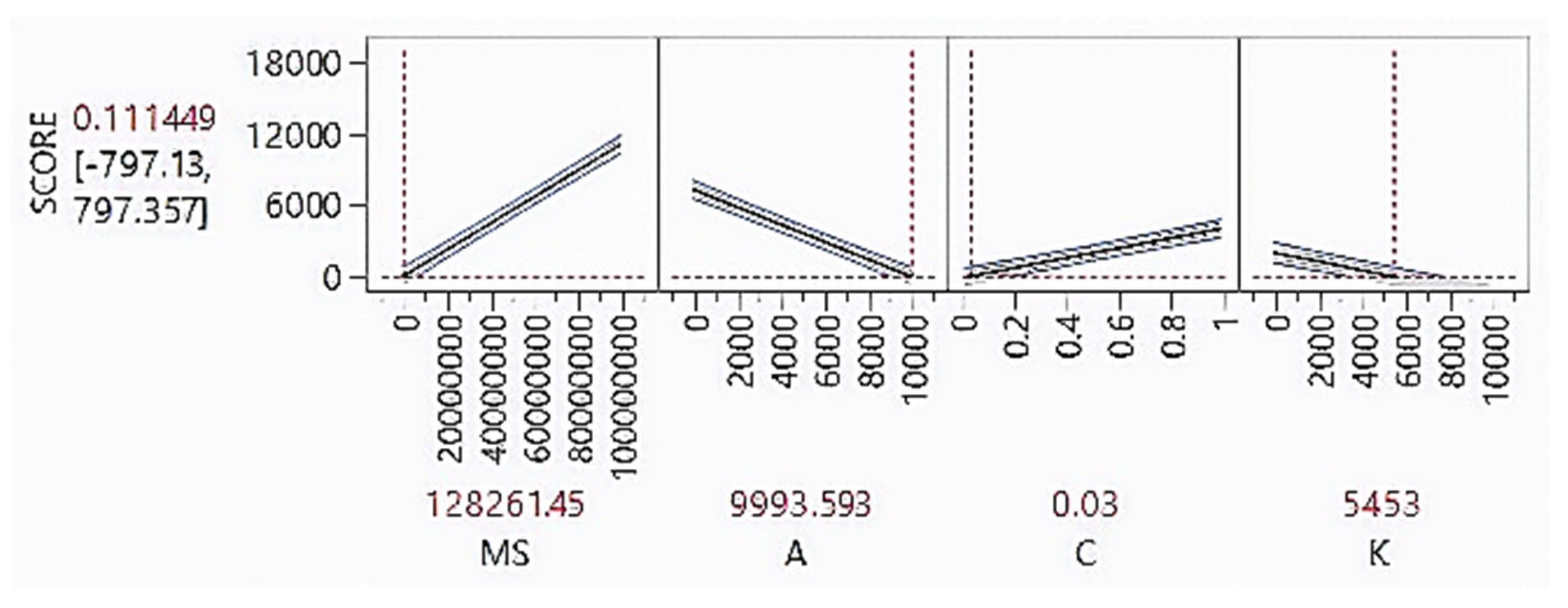
Table 1 of the Jiles Atherton model parameter, the larger its statistical significance and larger the slope of its response surface. The cross-hairs on the prediction profiler can be moved to reduce the response towards zero as much as possible. For example, reducing
MS and increasing
A would cause the response to move towards zero as shown in
Figure 3. This results in a SCORE (SSE) value of 0.111449, but with a wide confidence interval from −797.13 to 797.357.
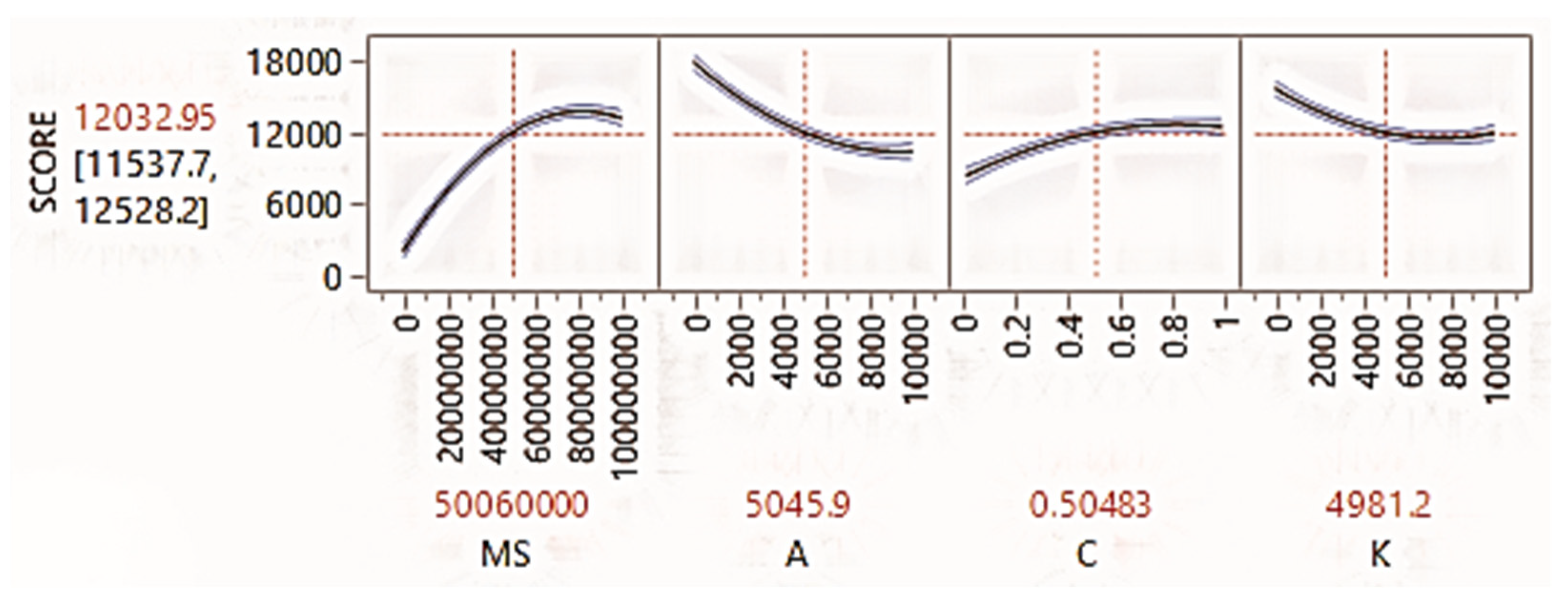
To improve the goodness of fit, we fit a response surface model (12) to check if there are any significant interactions or quadratic effects among the Jiles–Atherton model parameters.
As can be seen from
Table 2, as expected, all the Jiles–Atherton model parameters are significant to the SSE. However, the interaction effects between
MS and
C,
A and
K, and
C and
K are significant, too. Additionally, the quadratic effects of all the Jiles–Atherton model parameters are significant, too. The same is evident from the quadrature of the individual response surfaces in the prediction profiler, as can be seen in
Figure 4 and
Figure 5.
The goodness of fit of the response surface model, as measured by the metric RSquare Adjusted, is 0.84 or 84%. Since it is not a perfect fit i.e., 100%, we further explored the region near the values that give a zero response in the prediction profiler using stochastic optimization.
4. Parameter Identification of The Jiles–Atherton Model
Genetic algorithms [
17] are based on the theory of evolution. A population consists of individuals with genetic material called genes, which reproduce to create the next generation. Genes from two parent individuals are combined using various crossover procedures to create offspring individuals for the next generation and so on and so forth. The selection of individuals in the parent generation to reproduce is dependent on their fitness, i.e., their evaluation of the objective function of the optimization problem. Usually, the individuals with the best fitness move on to the next generation without reproduction in order to propagate the best solution through a process called elitism. Individuals that are not elite reproduce through crossover. To introduce variety in the genes, random changes are introduced into the genes of a fraction of the individuals in the offspring generation. This is analogous to mutation in evolution and helps in avoiding local minima in the optimization of the objective function. This evolution process continues until there is no improvement in the fitness in consecutive generations or until the predefined number of generations is reached.
The genetic algorithm was implemented with 50 individuals in each generation and 50 maximum generations. A crossover probability of 90% and a mutation probability of 5% was used. The full ranges in SPICE and the reduced ranges for each variable after the space-filling design are shown in
Table 3. The fitness function to be minimized corresponds to the total SSE between the actual and simulated transformer’s secondary voltage. The optimal values in those ranges as found by the genetic algorithm are also shown in the table. SAS JMP Pro 15 was used for the space-filling design, and MATLAB was used to implement the genetic algorithm and communicate with the SPICE simulator (OrCAD PSpice). The code required for conducting the approach is available in the
supplementary material. Due to the significant reduction (by about 85%) of the solution space of the Jiles–Atherton model parameters that the stochastic optimization algorithms have to explore, the computational time using this approach is significantly smaller than without the approach. The exact time required for the approach depends on the simulation time for the circuit of which the transformer is a part of.
This modeling technique was developed to be able to simulate a large analog circuit with five transformers. The Jiles–Atherton model parameters learnt by the proposed technique were used to implement the transformers in the SPICE circuit model. The circuit output as a result of the usage of these Jiles–Atherton model parameters was verified with the circuit output of the actual circuit. This procedure confirmed the validity of the developed method. Additionally, this procedure also speaks to the advantage of this technique —estimation of the Jiles–Atherton model parameters without resorting to the need for hysteresis parameter measurement.
5. Conclusions
This paper demonstrated a novel way to identify parameters for the Jiles–Atherton model. A space-filling design was used to search the solution space optimally, which is advantageous because the Jiles–Atherton model has multiple local minima. The overall method can ascertain Jiles–Atherton model parameters without having to use expensive hysteresis measurement devices. The only prerequisite for the application of this method is that the transformer’s secondary voltage (or current) waveforms must be known. This information can be measured by relatively inexpensive measurement devices.
Another advantage of this method is that it significantly reduces (by about 85%) the solution space of the Jiles–Atherton model parameters that the stochastic optimization algorithms have to explore. Additionally, by using space-filling designs, we have been able to discover previously unknown relations between Jiles–Atherton model parameters. For example, in addition to linear effects, the quadratic effects of the Jiles–Atherton model parameters are statistically significant at the 95% confidence level. We have observed that some of these interactions are also significant. A detailed simulation study is required to confirm these observations and possibly modify the Jiles–Atherton model to account for the new observations. This will be the focus of our future work.


