Determining the Correlation between Particulate Matter PM10 and Meteorological Factors

Abstract

In the article, we point out the need to measure the mass concentration of particulate matter (PM) in central Europe in a place of residence (a city and a small town), as PM has a negative impact on human health, especially that of children and the elderly. Since different amounts of PM (mainly peaks) were measured at two locations at a distance of 35 m from each other, a control measurement was also performed to verify the conformity of the measurements of both sensors, which was confirmed with measured courses of quantities. Cases of strong correlation (very close relationship) between PM10 and meteorological factors (temperature, humidity, barometric pressure) were found, but cases of no correlation were found as well, probably due to the effect of wind, which has not been measured yet. The article also points to the fact that, especially during the autumn/winter/spring heating season, the air quality in a small village may be worse than in a large city. This was also confirmed by the detected AQI sub-indices from PM2.5 and PM10. Due to the current rise in prices of gas and electricity, the use of wood combustion as a heating source is nowadays becoming increasingly more attractive, which may contribute to the worsening of the air quality in the future.

1. Introduction

Particulate matter (PM) consists of solid or liquid particles in the air of varying sizes and compositions. Particulate matter is categorized by its size, typically into the following categories: PM10 (particles with diameter <10 µm); PM2.5 or fine particles (<2.5 µm); coarse particles, which complement fine particles that are defined by diameter between 2.5 and 10 µm; and ultrafine particles or PM0.5 (<0.5 µm) [1]. The sources of PM can be natural (which include windblown dust, wildfires, volcano eruptions and sea salt aerosols) or anthropogenic [2,3]. The anthropogenic sources of PM include residential combustion, road traffic (more specifically, combustion from diesel and petrol engines, erosion of the pavement caused by the traffic as well as the abrasion of tires and brakes), and emissions from energy and manufacturing industries (metal processing, construction, manufacturing of cement and bricks, smelting and mining activities) [1,2,4].

The negative effects particulate matter has on health are well researched and documented. It is known that respiratory and cardiovascular systems are negatively affected by PM. The exposure to particulate matter can cause, for example, difficulty breathing, decreased pulmonary function, irregular heartbeat and is linked to asthma, heart attack and lung cancer [3,5,6,7,8]. In 2016, the World Health Organization estimated that 4.2 million premature deaths per year are due to exposure to ambient fine particles [9]. The smaller the particles are, the greater is their impact on human health; while coarse particles deposit in the upper respiratory system, fine particles can reach lung alveoli and ultrafine particles can even enter the bloodstream [10]. Particulate matter affects people of all ages, but children, the elderly, and pregnant women are amongst the most vulnerable [5,6,7,8]. There are no safe levels of PM mass concentration and the impact on human health is significant even for relatively low levels, which is the reason why we consider the measuring and monitoring of PM an important issue worth looking into. After all, to be able to lower the mass concentration of PM, we must first know how much particulate matter there is in the air. We are especially interested in finding if there is any significant correlation between the mass concentration of PM and other physical quantities, such as temperature, humidity, and barometric pressure. We are also interested in AQI calculated from daily averages of PM10 and PM2.5 mass concentrations. The previous research into the correlation between PM and meteorological factors such as temperature, humidity and pressure have found that favorable weather conditions, these conditions being sunny and warm weather as it was found that the increase in temperature helps reduce the concentration of air pollutants, and improve air quality as PM concentration relates significantly to meteorological factors [11,12,13,14]. Paper [11] has found negative correlation between PM concentrations and the average wind speed, precipitation and relative humidity, and positive correlation between PM concentration and barometric pressure. With the increase in the latitude, the impact of temperature on the air pollutant concentration became more obvious. The values of correlation coefficients between the concentration of air pollutants and meteorological conditions in autumn/winter were significantly higher than spring/summer. However, contrary to the findings of [11], the positive correlation between PM and humidity was also confirmed in [12], as the humidity causes the particles to become moist, which increases the weight of particles, which causes the reduction in the diffusion of particulate matter. The same study [12] also confirmed significant negative correlation between PM and barometric pressure, as well as between PM and the wind speed, as when no wind was present particulate matter tended to stick close to the ground. Furthermore, the same study found consistent negative correlation between temperature and PM concentration at different heights. The results of this study were obtained from the October–December period of measurement, which corresponds with the seasonal correlations found in the previous study [11]. Paper [13] found that the effect of meteorological factors (wind speed, temperature, air pressure, and relative humidity) on PM concentrations varied with each season. While wind speed was the most important factor, temperature, humidity and pressure have been found to be key factors during some seasons as well. Wind direction was also considered, and high and low PM concentrations were linked to different wind directions. In spring, air pollutants were more susceptible to the influences of temperature, wind speed and atmospheric pressure but not relative humidity. As in study [11], study [13] found that the correlation between PM and atmospheric pressure is positive as atmospheric pressure obstructs the upward movement of PM. This means that the higher the pressure, the more the particles accumulate, the higher the mass concentrations of PM in the air. In summer, the relative humidity was negatively correlated with PM mainly due to the low relative humidity during that season. Strong wind speeds in summer caused dust suspension, which caused the positive correlation between PM and wind speed. Wind speed was a key factor in the autumn season, when it was correlated negatively with PM, as it had important effect on pollutant diffusion. Just like in the autumn–winter season of [12], study [13] also found negative correlation between PM and temperature. In winter, PM was significantly positively correlated with humidity. Strong positive correlation between PM concentration and temperature was found by [12], though there was a long-term decrease in correlation coefficient in recent years (2010–2017). This suggests that the correlation between PM and meteorological factors varies with time. However, ref. [15] suggests that the effect of temperature on PM concentration is different during different months and during low temperatures (e.g., in December) it is correlated with PM negatively. Study [16] found regional differences in correlations between PM2.5 and meteorological factors. Temperature was positively correlated with PM concentrations throughout the US. The correlation of PM with relative humidity varied with different regions—it was positive in the Northeast and Midwest but negative in the Southeast and the West. It was found that precipitation was negatively correlated with PM throughout the US. A study conducted in the Czech Republic [17] was to characterize vertical distribution of PM in spring and summer. Meteorological factors were measured simultaneously with PM. Strong correlation between PM and meteorological factors were not found.

Studies [11,12,13,15] were conducted in China. Study [12] was conducted in South Korea and study [16] was conducted in the US. We hope that this paper finds how PM is affected by the meteorological factors in central Europe. The weather conditions in central Europe are different than those in East Asia or the United States, which may affect the concentration of PM in different ways. Our study is conducted in Košice (a city), and in a small village located 35 km from Košice. Considering the aforementioned negative effects on human health, we were interested in the state of air quality. This was reflected in PM concentrations in the form of graphs, and AQI in the form of numerical values. Additionally, correlation between PM and meteorological factors (temperature, humidity, pressure) was calculated, which could help with the future predictions of PM mass concentration.

In short, this paper has the following objectives:

• measure the mass concentration of PM, calculate AQI for PM2.5 and PM10;
• compare air quality in a city and in a small village;
• compare the air quality within short distances relative to the sources of PM;
• calculate the correlations between PM and meteorological factors (temperature, humidity, pressure).

2. Materials and Methods

2.1. Measurement Station

To measure particulate matter, a measurement station was created. The station was based on the Arduino Mega board, to which several sensors have been connected along with the Real Time Clock (RTC) module and a microSD module. The sensors used in the measuring station were the following: particulate matter sensor SPS30, which measures mass concentration of PM1, PM2.5, PM4 and PM10, quantity of particles of PM0.5, PM1, PM2.5, PM4 and PM10 and typical size of the particles. SPS30 is an OPC (optical particle counter) based on the principle of laser diffraction. The particle intercepts the laser beam, which causes the beam to scatter. The scattered light is then measured by the photodetector. The intensity of the scattered light allows the individual particles to be counted and measured. The sensor measures mass concentration of PM1 and PM2.5 with the accuracy of ±10 µg/m³ for mass concentration < 100 µg/m³ and ±10% for mass concentration > 100 µg/m³. Mass concentration of PM4 and PM10 is measured with the accuracy of ±25 µg/m³ for mass concentration < 100 µg/m³ and ±25% for mass concentration > 100 µg/m³ [18]. The next sensor used in this measurement station was the temperature and humidity sensor SHT30, which measures temperature with the accuracy of ±0.3 °C and humidity with the accuracy of ±3% RH [19]. The final sensor used in this measurement station was the temperature and pressure sensor MS5611. It measures temperature with the accuracy of ±0.8 °C and pressure with the accuracy of ±1.5 hPa [20]. The measurements were taken every 5 s and saved in a *.csv file on a microSD card. The RTC module assured the measurements were properly timestamped.

2.2. Test Measurement of SPS30

In order to verify that the measured values of the two SPS30 sensors do not significantly differ from each other, a test measurement (Figure 1) has been conducted, for which two SPS30 sensors were used simultaneously.

Figure 1a,b depict the measured values by both SPS30 sensors. 15,784 measurements were made over the course of ~22 h. Experimental data from this measurement are available in Table S1, Supplementary Materials. From these two graphs it is not apparent just how many values measured by S1 differ from the values measured by S2, therefore the difference between these values is plotted in Figure 1c. Most of the time, when the mass concentration of PM10 is ~5 µg/m³, the difference between measurements of S1 and S1 falls between −1 and +1 µg/m³. The exceptions happen during the 20–25 µg/m³ peaks, when the difference between S1 and S2 measurements is 3–4 µg/m³. In all cases, this difference is less than 10 µg/m³, which means that both sensors comply with the accuracy guaranteed by the manufacturer [15]. The scatter plot of the difference between S1 and S2 is shown in Figure 1d.

The reason it is important to evaluate the accuracy of the sensor used for measuring PM is due to the negative effects of particulate matter on human health, as described in the Introduction. In our experience with different sensors, we have come across sensors that did not meet the accuracy guaranteed by the manufacturer. An example of one such sensor is temperature and barometric pressure sensor BMP280, which measures temperature with the accuracy of ±1 °C and barometric pressure with the accuracy of ±1.7 hPa [21]. During our previous work with this type of sensor, we used eight BMP280 sensors to simultaneously measure temperature and pressure, as shown in Figure 2. Measured data by BMP280 sensors are available in Table S2, Supplementary Materials.

As shown in Figure 2a the difference between S5 (which recorded the highest temperature) and S4 (which recorded the lowest temperature) is ~5 °C. Figure 2b shows that S8 (highest recorded pressure) and S1 (lowest recorded pressure) differ by 160 hPa. While the barometric pressure deviated from the accuracy of the sensor by a significantly greater margin, neither the temperature nor the pressure correspond to the accuracy guaranteed by the manufacturer.

However, seeing as there was no such problem in the case of SPS30 (as demonstrated by Figure 1), we have concluded that this sensor is reliable for our measurements of PM, temperature, humidity, and barometric pressure.

2.3. Measurement Locations

The measurements of PM took place over the course of several months (in this article we will include measurements from January, March and May 2022) in multiple locations.

The first set of measurements took place in Slovakia, in Košice at the Department of Theoretical Industrial Electrical Engineering, and was carried out in November and December 2021 [22]. The measurement station was placed outside of a window on the first floor of the building. A park was situated just across the road from this area, and the measuring station was facing the park. The road itself was not often busy, as it was located in the university campus and the nearest four-lane main road was situated 150 m from the department, behind a park, which filtered PM created by traffic.

The second set of measurements was conducted in a small village, on one street with five family houses clustered together as a close neighborhood. All of them used wood combustion as a primary heat source (although one of them could also use gas for heating), which is understandably increasingly attractive, even for the houses which also had the option to heat using gas or electricity due to rising energy prices. The measurements were carried out simultaneously in two places—on the balcony of the house and in the garden on the other side of the same house. The distance between both measuring places was 35 m.

2.4. Data Collection and Processing

The measurements in both locations were carried out in 5-s intervals, which means that there are 2160 measured values in a 3-h interval, 4320 measured values in a 6-h interval and 8640 measured values in a 12-h interval.

The measured data was logged into a *.csv file on a microSD card, after which MATLAB software was used to process the data. The measured data was divided into 3-h, 6-h and 12-h intervals, from which correlation coefficients were calculated. In addition, hourly averages of PM were calculated for the 12-h intervals and plotted in bar graphs. Daily averages of PM were also calculated, which were necessary for calculating AQI values. All graphs were plotted using MATLAB.

2.5. Calculating AQI

Air Quality Index (AQI) indicates the levels of air pollutants from a public health point of view. It evaluates the impact of air pollutants on human health. A number of air pollutants are taken into consideration when calculating AQI: PM2.5, PM10, CO, SO₂, NO₂ and O₃.

Table 1. AQI categories and their corresponding levels of air pollutants. Adapted from [24].

O3 ** (ppm)	O3 *** (ppm)	PM2.5 * (µg/m3)	PM10 * (µg/m3)	CO ** (ppm)	SO2 *** (ppb)	NO2 *** (ppb)	AQI	Category
0.000–0.054	-	0.0–12.0	0–54	0.0–4.4	0–35	0–53	0–50	Good
0.055–0.070	-	12.1–35.4	55–154	4.5–9.4	36–75	54–100	51–100	Moderate
0.071–0.085	0.125–0.164	35.5–55.4	155–254	9.5–12.4	76–185	101–360	101–150	Unhealthy for sensitive groups
0.056–0.105	0.165–0.204	55.5–150.4	255–354	12.5–15.4	186–304	361–649	151–200	Unhealthy
0.106–0.200	0.205–0.404	150.5–250.4	355–424	15.5–30.4	305–604	650–1249	201–300	Very unhealthy
-	0.405–0.504	250.5–350.4	425–504	30.5–40.4	605–804	1250–1649	301–400	Hazardous
-	0.505–0.604	350.5–500.4	505–604	40.5–50.4	805–1004	1650–2049	401–500	Hazardous

* 24-h average. ** 8-h average. *** 1-h average.

shows the categories of AQI and what level of air pollutants correspond to them [23,24]. AQI can be characterized by one of 6 categories: Good, Moderate, Unhealthy for sensitive groups (sensitive groups are defined for each air pollutant in

Table 2. AQI categories and their corresponding levels of air pollutants. Adapted from [24].

Air Pollutant	Sensitive Groups
O3	People with lung disease, children, older adults, people who are active outdoors (incl. outdoor workers), people with certain genetic variants, and people with diets limited in certain nutrients
PM2.5 and PM10	People with heart or lung disease, older adults, children, and people of lower socioeconomic status
CO	People with heart disease
SO2 and NO2	People with asthma, children, and older adults

), Unhealthy, Very unhealthy and Hazardous.

AQI sub-indices [24] are calculated for each air pollutant using the following equation:

$$I_p=\frac{I_{Hi}-I_{Lo}}{B{P}_{Hi}-B{P}_{Lo}}\left(C_p-B{P}_{Lo}\right)+I_{Lo},$$

(1)

where I_p = index for pollutant p, C_p = truncated concentration of pollutant p, BP_Hi = concentration breakpoint greater than or equal to C_p, BP_Lo = concentration breakpoint less than or equal to C_p, I_Hi = AQI value corresponding to BP_Hi, I_Lo = AQI value corresponding to BP_Lo.

From then, the final AQI [24] is determined as:

$$\mathrm{AQI}=\max \left({\mathrm{I}}_{\mathrm{PM}2.5},{ \mathrm{I}}_{\mathrm{PM}10},{\mathrm{I}}_{{\mathrm{O}}_3},{\mathrm{I}}_{\mathrm{CO}},{\mathrm{I}}_{{\mathrm{SO}}_2},{\mathrm{I}}_{{\mathrm{NO}}_2}\right).$$

(2)

However, since only PM2.5 and PM10 were measured, we can only calculate the sub-indices I_PM2.5 and I_PM10. This still has an informational value for us, as it can tell us which parts of the PM have higher impact on the air quality and what that air quality is, at least with respect to PM.

2.6. Post-Hoc Test for Determining Statistical Significance

Our null hypothesis is that there is no significant correlation between PM and other meteorological factors:

$$H_0: \rho =0.$$

(3)

The formula for the test statistic is:

$$t=\frac{r\sqrt{n-2}}{\sqrt{1-r^2}},$$

(4)

where r = correlation coefficient between two quantities, n = sample size.

p-value then can be calculated using an MS Excel function = TDIST(t, n − 2, 2), where t is a value of test statistic calculated by Equation (4), n is the sample size and 2 indicates 2-tailed test. If p ≤ α, we reject the null hypothesis, thus concluding that the non-zero correlation found between the pair of measured quantities is statistically significant. If p > α, null hypothesis cannot be rejected.

With small datasets, it is customary to use α = 0.05. However, we deal with large datasets (n = 2160 for 3-h intervals, n = 4320 for 6-h intervals, n = 8640 for 12-h intervals), so the significance threshold α needs to be scaled by a bandwidth, which can also be adjusted to account for multiple comparisons, a solution offered by Naaman [25]. The scaled significance threshold α is shown in

Table 3. Significance threshold α scaled according to sample size n.

Interval Length	n	α
3 h	2160	1.072 × 10−7
6 h	4320	2.679 × 10−8
12 h	8640	6.698 × 10−9

.

3. Results

3.1. Measurements in Košice, Slovakia

During the first set of measurements (in Košice, Slovakia, at the Department of Theoretical and Industrial Electrical Engineering, data available in Table S3, Supplementary Materials) it was found that the air quality with respect to mass concentration of PM is usually (other than in a few exceptions) very good (VG) or good (G), as per

Table 4. Limit values for hourly averages of PM2.5 and PM10 mass concentrations. Adapted from [26].

Air Quality	Hourly Average of PM2.5 (µg/m3)	Hourly Average of PM10 (µg/m3)
Very Good (VG)	0–14	0–20
Good (G)	14–25	20–40
Worsened (W)	25–70	40–100
Bad (B)	70–140	100–180
Very Bad (VB)	140+	180+

[26].

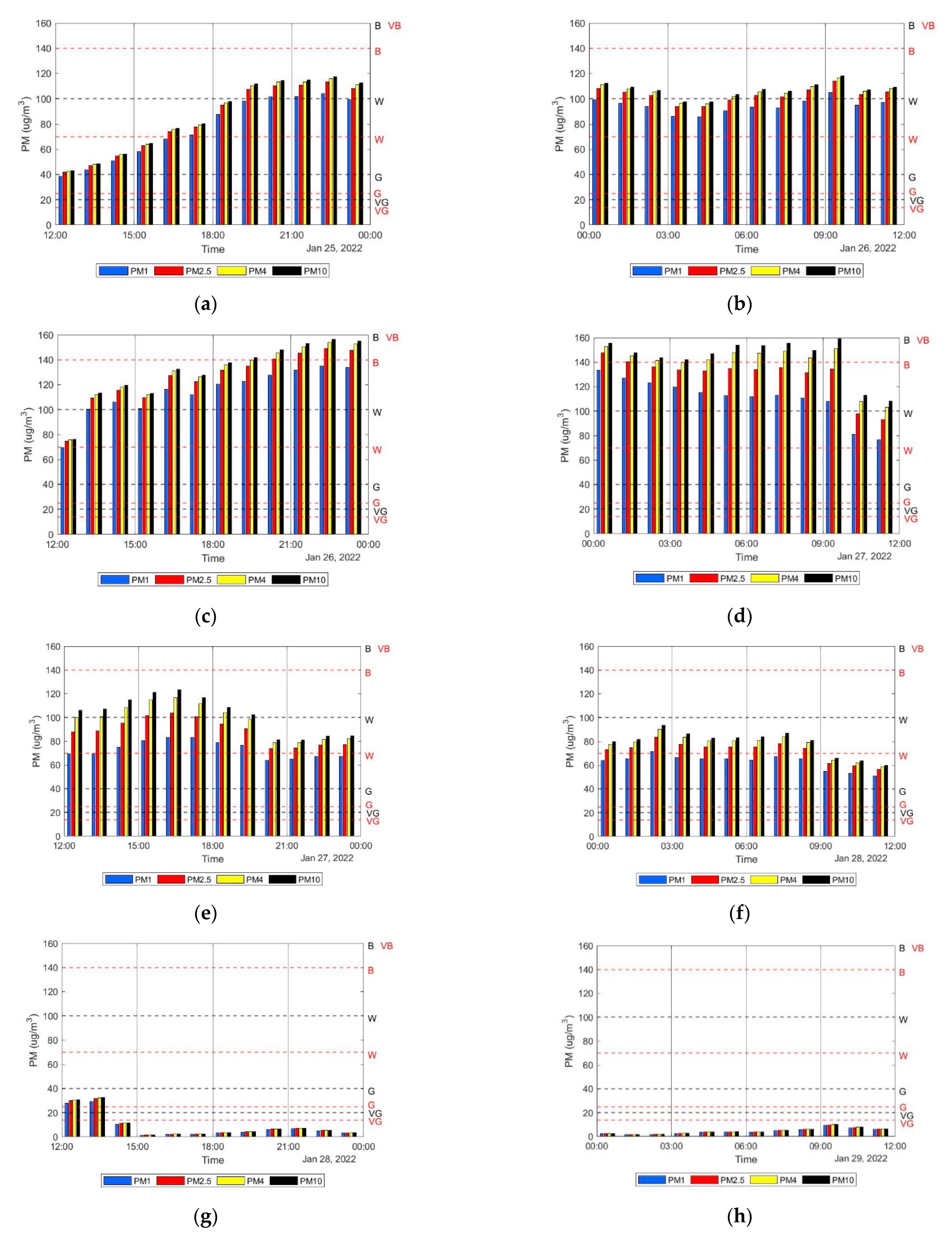
Good air quality was also confirmed by the measurements conducted in January 2022 up until 25 January, when during the afternoon hours (Figure 3a), the mass concentration of PM started to steadily increase. The hourly average of PM10 mass concentration increased from ~40 µg/m³ at 12:00 to 110 µg/m³ at 19:00. The mass concentration stays roughly the same for the next 12 h (Figure 3b). It momentarily dips to ~80 µg/m³ at 12:00 on 26 January 2022 (Figure 3c), before it rises to ~160 µg/m³ by 22:00. PM10 mass concentration then reaches 140–160 µg/m³ for the next 11 h (Figure 3d). However, it is important to note that mass concentration of PM1 starts falling during this period of time. The increase in PM10 compared to PM1 at 9:00 to 10:00 (Figure 3d) is almost 50%, which only happens sometimes (during these measurements and also on 27 January at 15:00 to 18:00—Figure 3e). From 27 January 2022 at 22:00, the concentration of particulate matter (all measured categories) starts decreasing (Figure 3d–g), until it reaches the hourly average of 1 µg/m³ on 28 January 2022 at 15:00, after which the mass concentration stays in the category of very good (VG) air quality levels. The decrease in mass concentration at 11:00–15:00 (Figure 3f,g) is significant. The levels of mass concentration of particulate matter as measured on 25 to 28 January 2022 12:00 (Figure 3a–f) are not typical for this location. Measurements carried out on 28 January 2022 12:00 and onwards (Figure 3g,h) are much closer to the mass concentration, which is usually measured at the Department of Theoretical and Industrial Electrical Engineering (DTIEE), FEEI, TU of Košice.

AQI was calculated from the daily averages of PM2.5 and PM10 for the better understanding of air quality. Table 1 contains the AQI categories characterized by the levels of concentration of different air pollutants (PM2.5, PM10, CO, O₃, SO₂ and NO₂) [23,24]. AQI sub-indices for each pollutant are calculated using Equation (1). The resulting AQI is equal to the maximum value of the AQI sub-indices. Since only PM was measured and no other air pollutants, the overall AQI cannot be determined. However, the I_PM2.5 and I_PM10 can be calculated, and they do carry an informative value of how PM impacts air quality and which PM has greater impact.

Table 5. Air Quality Index for Košice, DTIEE measurement.

Date	PM2.5 * (µg/m3)	IPM2.5	PM10 * (µg/m3)	IPM10
25 January 2022	72.3	160	75	60
26 January 2022	115.4	182	120	83
27 January 2022	109.1	179	123	85
28 January 2022	40.7	114	44	41
29 January 2022	7.2	30	7	7

* 24-h average.

consists of daily averages of PM2.5 and PM10 and their respective AQI sub-indices. For three days (25 to 27 January 2022), the air quality is unhealthy. On 28 January 2022 the air quality is unhealthy for sensitive groups. However, on 29 January 2022 the air quality finally reaches good levels. In all cases, I_PM2.5 negatively influenced the air quality to a greater degree than I_PM10, which is also the case in the following measurements in March 2022 (Section 3.2). Nevertheless it should be noted that this long term increase (lasting about four days) in PM mass concentration is rare in Košice at DTIEE, as we have found that the PM mass concentration measured on 29 January 2022 is much more true to the usual levels (as has been found in our previous measurements in [22]).

The measurements were divided into 12-h (for which the hourly averages of PM mass concentration were calculated and visualized in Figure 3), 6-h and 3-h long intervals. For each interval correlation coefficients between all possible pairs of measured quantities were calculated. In the following tables we present r between PM10 and temperature, humidity, and pressure. Correlation coefficients during the 12-h intervals are shown in

Table 6. Correlation between mass concentration of PM10 and temperature, humidity, pressure: 12-h intervals.

Interval	PM10 and Temperature	PM10 and Humidity	PM10 and Pressure
25 January, 12:00–24:00	−0.931	0.941	−0.703
26 January, 0:00–12:00	0.281	−0.232	−0.003 **
26 January, 12:00–24:00	−0.853	0.874	−0.858
27 January, 0:00–12:00	−0.652	0.527	0.514
27 January, 12:00–24:00	−0.304	0.165	0.563
28 January, 0:00–12:00	−0.859	0.791 *	−0.447
28 January, 12:00–24:00	0.574	−0.366	−0.590
29 January, 0:00–12:00	0.443	−0.474	0.651

* r close to lower limit of moderate correlation (number in white cells) or strong correlation (light grey cells). ** r, for which p > α.

; 6-h intervals in

Table 7. Correlation between PM10 and temperature, humidity, pressure: 6-h intervals.

Interval	PM10 and Temperature	PM10 and Humidity	PM10 and Pressure
25 January, 12:00–18:00	−0.955	0.940	−0.680
25 January, 18:00–24:00	−0.562	0.710	−0.443
26 January, 0:00–6:00	−0.701	−0.229	0.410
26 January, 6:00–12:00	0.125	−0.097	0.484
26 January, 12:00–18:00	−0.915	0.731	−0.736
26 January, 18:00–24:00	−0.780	0.835	−0.778
27 January, 0:00–6:00	−0.394 *	0.373	0.388 *
27 January, 6:00–12:00	−0.725	0.672	0.599
27 January, 12:00–18:00	−0.432	0.342	−0.428
27 January, 18:00–24:00	−0.527	0.176	0.751
28 January, 0:00–6:00	−0.301	0.030 **	−0.348
28 January, 6:00–12:00	−0.913	0.910	−0.813
28 January, 12:00–18:00	0.695	−0.260	−0.792 *
28 January, 18:00–24:00	−0.340	0.615	0.101
29 January, 0:00–6:00	−0.435	−0.388 *	0.854
29 January, 6:00–12:00	0.507	−0.422	0.205

* r close to lower limit of moderate (number in white cells) or strong correlation (light grey cells). ** r for which p > α.

; and 3-h intervals in

Table 8. Correlation between PM10 and temperature, humidity, pressure: 3-h intervals.

Interval	PM10 and Temperature	PM10 and Humidity	PM10 and Pressure
25 January, 12:00–15:00	−0.847	0.922	−0.815
25 January, 15:00–18:00	−0.900	0.747	0.096 **
25 January, 18:00–21:00	−0.721	0.723	−0.267
25 January, 21:00–24:00	−0.632	0,369	0.077 **
26 January, 0:00–3:00	−0.220	−0.497	0.573
26 January, 3:00–6:00	−0.595	0.719	−0.605
26 January, 6:00–9:00	0.473	−0.413	0.710
26 January, 9:00–12:00	−0.715	0.744	0.225
26 January, 12:00–15:00	−0.941	0.683	−0.707
26 January, 15:00–18:00	−0.896	0.739	−0.553
26 January, 18:00–21:00	−0.780	0.804	−0.688
26 January, 21:00–24:00	−0.284	0.369	−0.232
27 January, 0:00–3:00	−0.399 *	0.555	0.641
27 January, 3:00–6:00	−0.701	0.726	0.120
27 January, 6:00–9:00	−0.350	0.357	0.244
27 January, 9:00–12:00	−0.862	0.846	0.343
27 January, 12:00–15:00	−0.438	0.440	−0.371
27 January, 15:00–18:00	−0.634	0.398 *	0.019 **
27 January, 18:00–21:00	−0.888	0.625	0.779
27 January, 21:00–24:00	−0.481	0.460	−0.492
28 January, 0:00–3:00	−0.467	0.078 **	−0.863
28 January, 3:00–6:00	0.018 **	−0.289	0.221
28 January, 6:00–9:00	−0.601	0.550	−0.591
28 January, 9:00–12:00	−0.653	0.689	−0.018 **
28 January, 12:00–15:00	0.350	0.858	−0.823
28 January, 15:00–18:00	−0.558	0.597	0.574
28 January, 18:00–21:00	−0.417	0.606	0.591
28 January, 21:00–24:00	−0.555	0.639	−0.440
29 January, 0:00–3:00	0.264	0.589	0.030 **
29 January, 3:00–6:00	−0.757	−0.207	0.832
29 January, 6:00–9:00	0.444	−0.249	0.784
29 January, 9:00–12:00	0.364	−0.136	0.368

* r close to lower limit of moderate (number in white cells) or strong correlation (light grey cells). ** r for which p > α.

. The cells in Table 6, Table 7 and Table 8 with corresponding correlation coefficient (r) are shaded in three colors. White color indicates weak correlation (|r| < 0.4) (or no correlation, when r approaches 0); light grey indicates moderate correlation (0.4 < |r| < 0.8) and dark grey indicates strong correlation (|r| > 0.8) [27]. The asterisk marks r close to the lower limit of moderate or strong correlation.

As can be seen from Table 6, there are only four measurements with weak correlation and one with none. The rest of the measurements show correlation; most of them moderate but some show strong correlation (ex. |r| = 0.93–0.94, a very close relationship between the measured quantities). The first row (25 January, 12:00–24:00) indicates strong correlation between PM10 and Temperature, and Humidity; and moderate correlation between PM10 and pressure. In the 2nd row, there is a weak correlation on 26 January, 0:00–12:00. Furthermore, r for PM10 and Pressure equals −0.003 (no correlation).

After performing a post-hoc test to get the adjusted p-values (two-tailed, n = 8640), it was found that all except for one p-value were less than α (as corresponding to Table 3).

After dividing the 12-h interval ex. of the second row from Table 6 (26 January, 0:00–12:00) into 6-h intervals (Table 7), it is apparent that out of six correlation coefficients, three show moderate correlation (between PM10 and Pressure, during the 0:00–6:00 and 6:00–12:00 intervals and between PM10 and Temperature during the 0:00–6:00 interval). This finding is interesting, since r between PM10 and Pressure was close to zero during the 12-h interval, while the 6-h intervals both show moderate correlation.

All p-values (two-tailed, n = 4320) except for one in Table 7 were equal to or lesser than α (as corresponding to Table 3).

Even more interesting is the case when the same 12-h interval from Table 6 is divided into four 3-h intervals, which means 12 correlation coefficients will be calculated. Table 8 shows that out of all 3-h intervals, only three of them show weak or no correlation for all the physical quantities (white cells of the table) and the rest of the interval shows mostly moderate correlation. Another surprise in Table 7 and Table 8 is that for the first row in Table 6 (25th January, 12:00–24:00), r for PM10 and Pressure during the 12-h interval is −0.703, while for the 6-h intervals r = −0.681 and −0.443. The biggest surprise was dividing the 12-h interval into 3-h intervals, as in Table 8, for 25th January, 12:00–15:00 r = −0.815 and the other three intervals show no correlation (r ≈ 0). It is possible to observe the development of r for other measurements in Table 8 in a similar way.

All except for seven p-values (two-tailed, n = 2160) were equal to or lesser than α (as corresponding to Table 3).

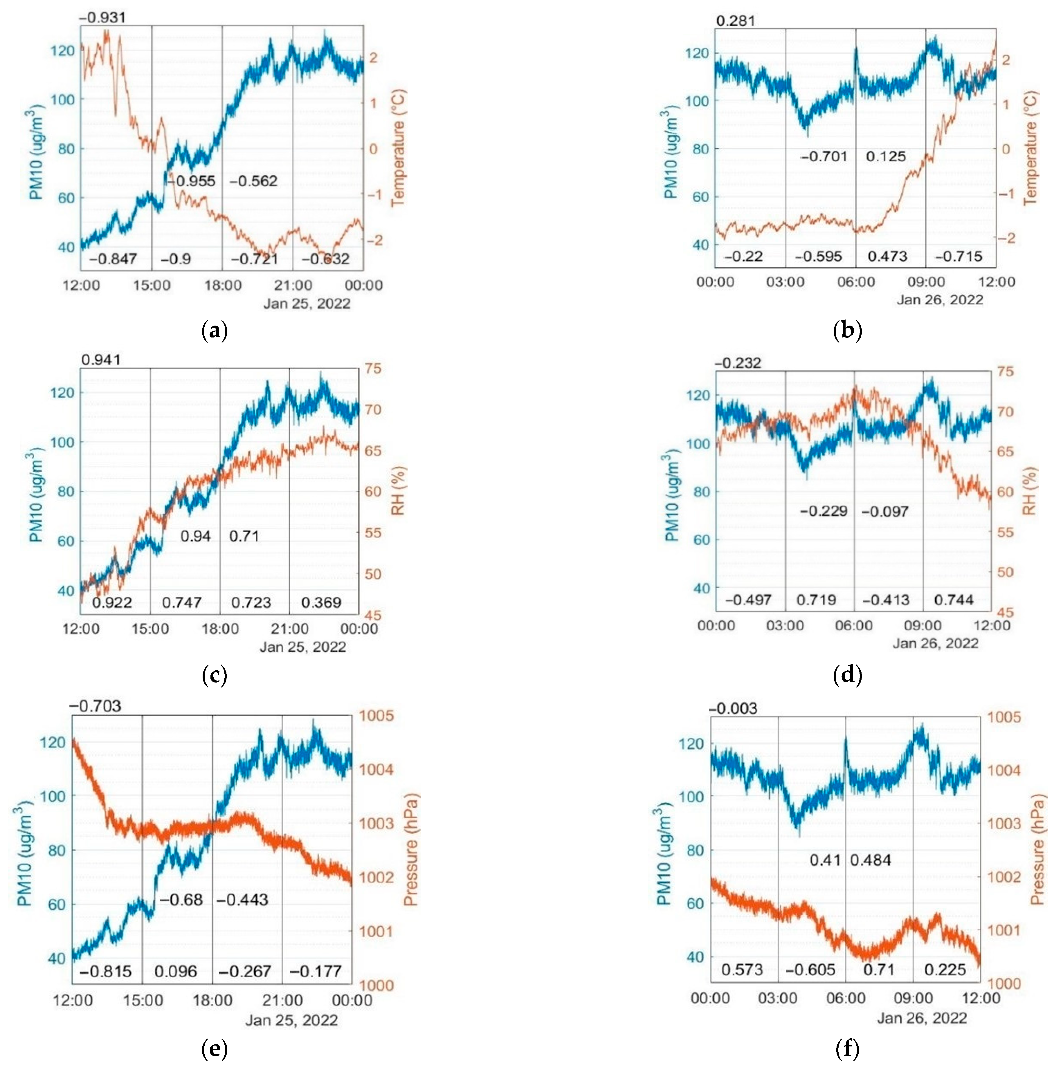
We were interested in finding what the changes were in measured quantities that correspond to r calculated for the intervals in Table 6, Table 7 and Table 8. Figure 4 illustrates the changes in measured quantities over 12 h for the first and second row in Table 6. Since the positive and negative correlations are indicated in the tables, it will be possible to observe the increase or decrease in both measured quantities in the case of positive r, or the increase in one and the decrease in the other measured quantity in the case of negative r. The timeline in Figure 4 is divided into 3-h intervals, which means it will be possible to observe the change in measured quantities and r corresponding not only for the 12-h intervals, but also for the 6-h and 3-h intervals.

The numbers written on the bottom of the graphs inside the 3-h intervals are the corresponding correlation coefficients from Table 8 for the 3-h intervals. The numbers written in the middle of the graph next to the 6-h line are the corresponding r from Table 7 for the 6-h intervals and the number written in the top left corner of the picture is the corresponding r from Table 6 for the 12-h interval. In the left column, all the graphs show the measured quantities on 25th January, 12:00–24:00 and in the right columns, the graphs show the measured quantities on 26th January 0:00–12:00. The first row shows the changes in mass concentration of PM10 and Temperature, and the second row shows the changes in mass concentration of PM10 and Humidity. Finally, the 3rd row shows the changes in mass concentration of PM10 and Pressure.

In Figure 4a it is apparent why r = −0.931. The increase in PM10 mass concentration corresponds to the decrease in temperature, which is why r is of such high value with a negative sign. Similarly, in Figure 4c, the increase in PM10 mass concentration corresponds to the increase in Humidity, so r = 0.941 with a positive sign. Figure 4e is an answer to why r = −0.703 for correlation between PM10 and Pressure. The barometric pressure is almost constant from 14:00 to 19:00 and it is the reason r is not close to the value of −0.9, even though for the 3-h interval from 12:00 to 15:00, r = −0.815. On the other hand, in Figure 4f r = −0.003 for the 12-h interval. However, for the 3-h or 6-h intervals r shows moderate correlation between PM10 and pressure. Other graphs in Figure 4 can be described in a similar way.

The question which arose from these measurements is: why is there not always at least moderate correlation between PM10 and other quantities? Why does the value of r change significantly with each interval? If there was a relationship found between the mass concentration of particulate matter and other quantities, it would be possible to predict the future development of mass concentration of PM and therefore warn the population against the high concentration of PM in the air. Mass concentration of PM could be forecast similarly to weather. The air pollution by particulate matter changes not only with temperature, humidity, and pressure, but also with wind speed and direction [12,13]. Unfortunately, comparing the measured data with the wind speed and direction data has not yet been implemented in our measuring station due to a lack of availability of components or long delivery times needed for extending our measuring station with an anemometer.

3.2. Measurements in a Small Village

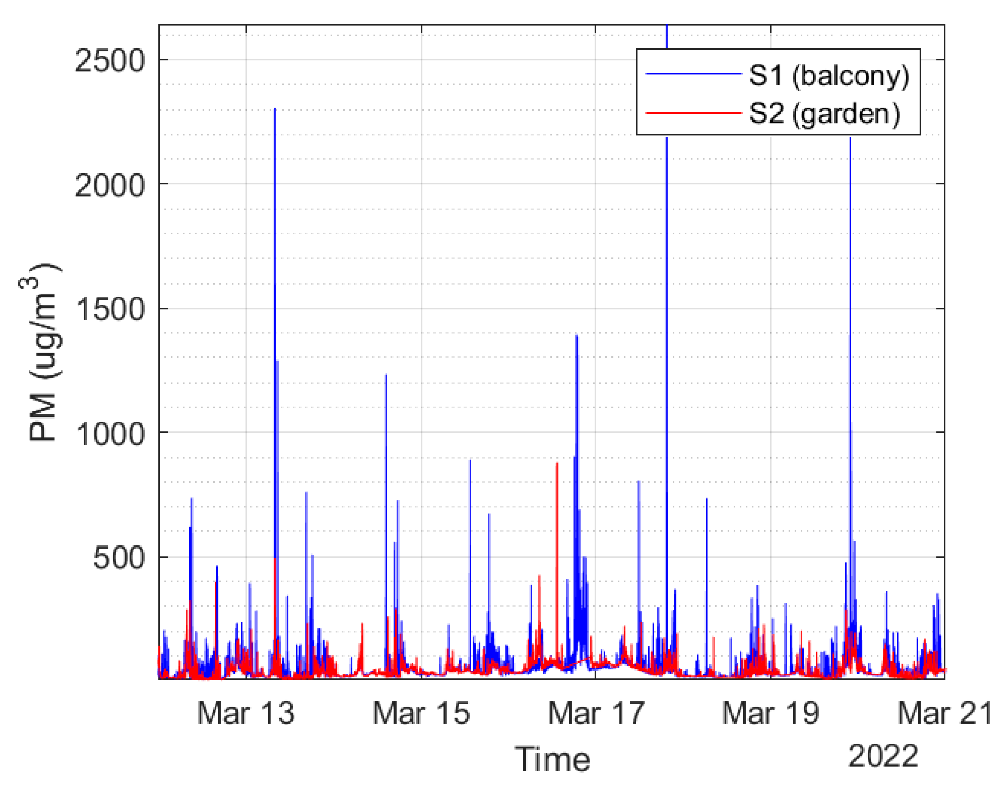
Another question is whether the place of measurement also affects the mass concentration of PM, and if so, to what degree. Therefore, a second set of measurements (Figure 5) was carried out in a small village (the place of measurement described in 2.3. Measurement Locations). Measured data are available in Tables S4–S6, Supplementary Materials.

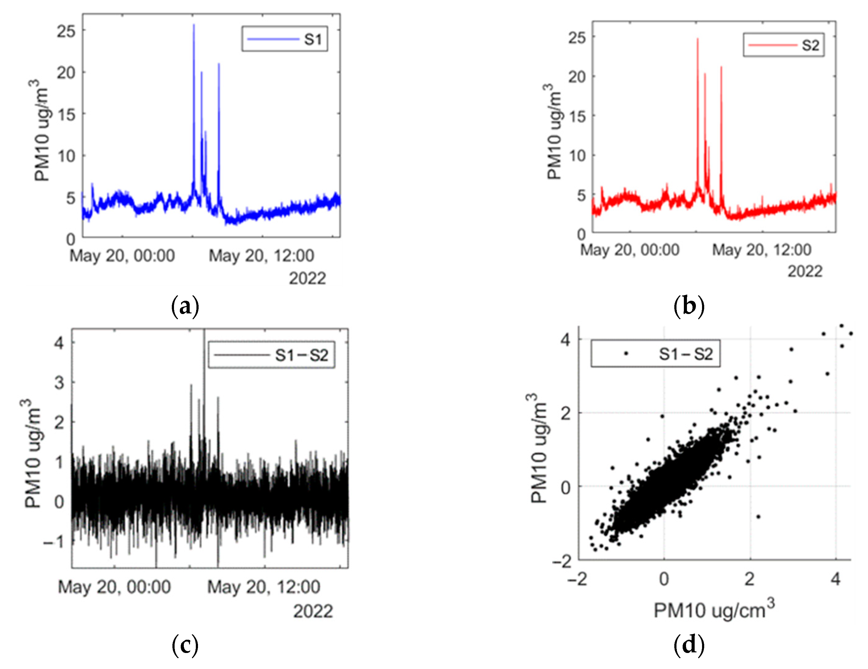
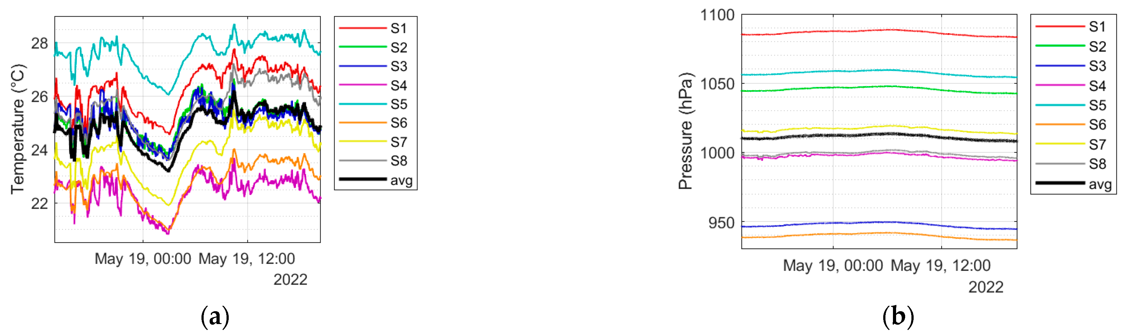
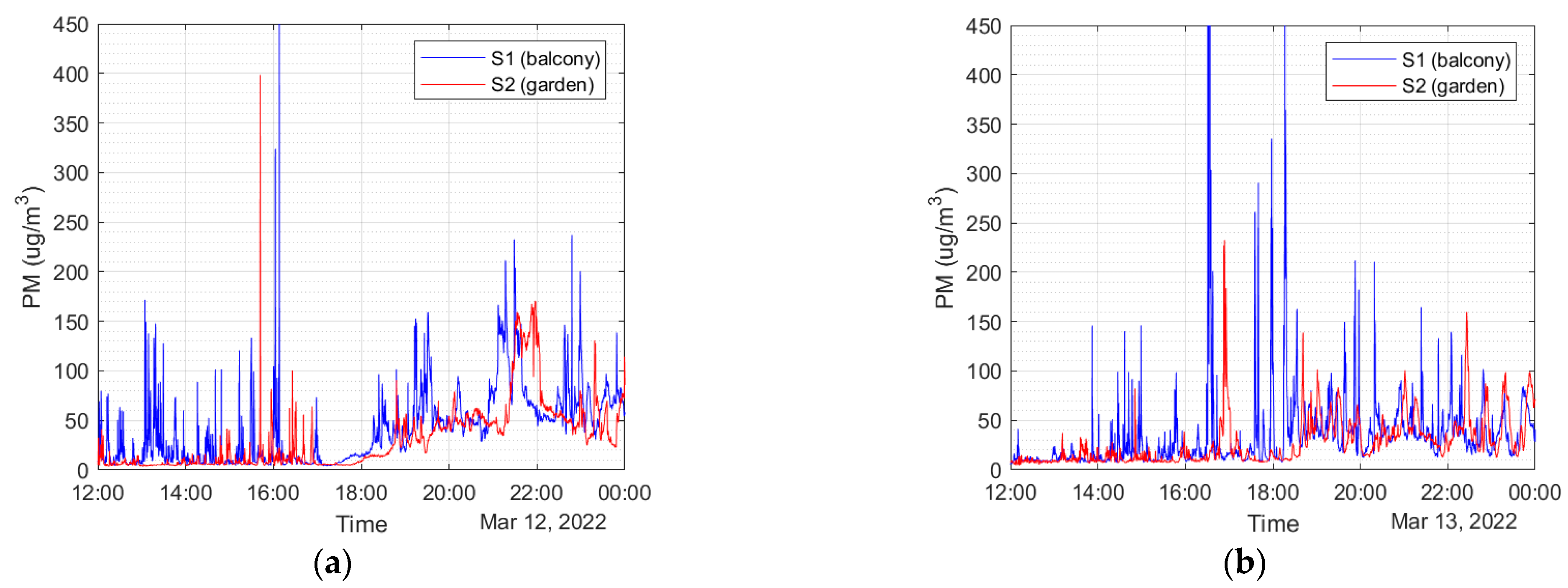
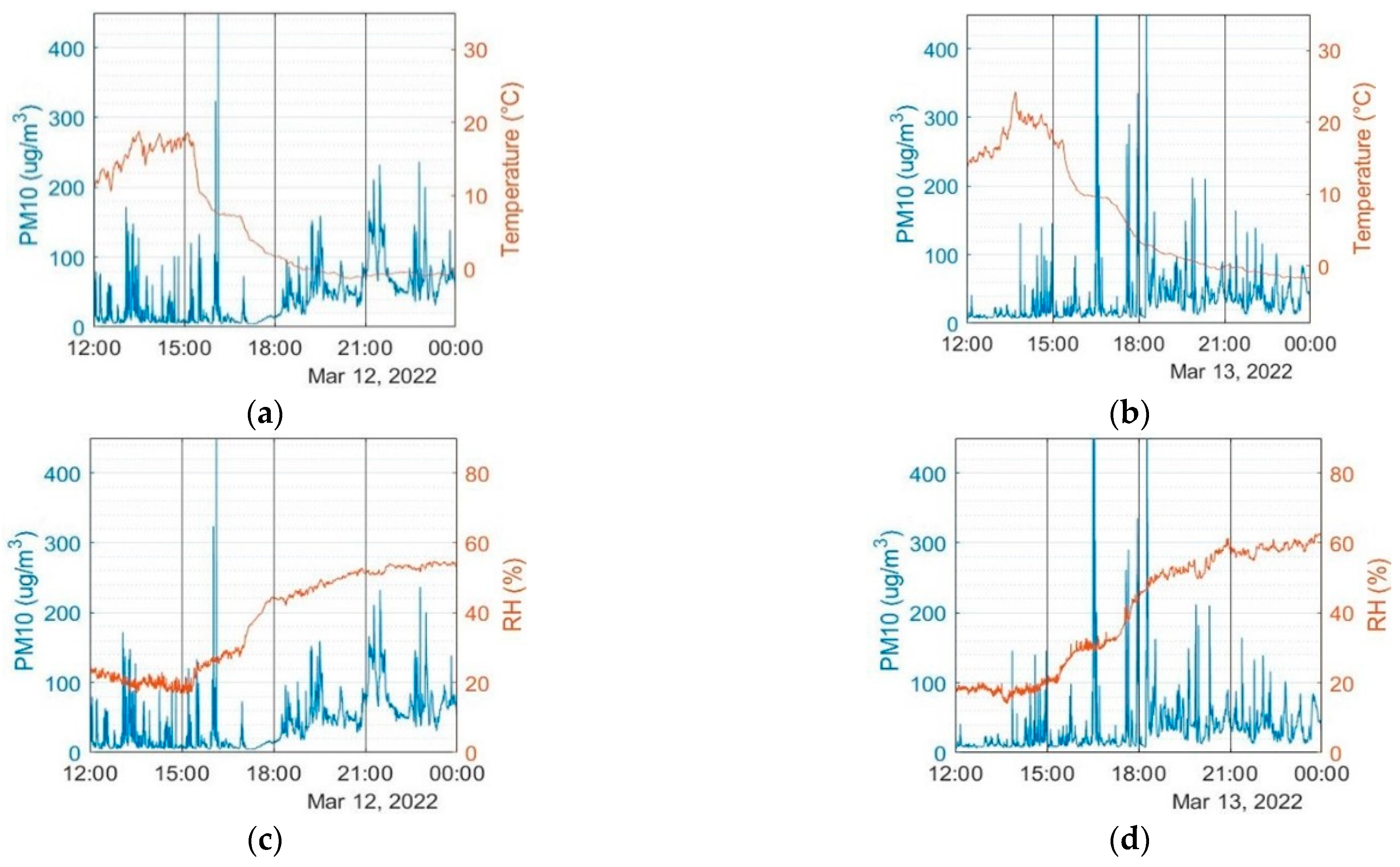
As it can be seen in Figure 5, values measured by sensor S1 on the balcony and sensor S2 in the garden differ. The most noticeable differences are during short-term peaks in mass concentration of PM10. For a better view, Figure 6 shows a close-up on the 12:00–24:00 intervals on 12th (Figure 6a) and 13th March (Figure 6b). It is important to note, that while the y-axis scale is set to 450 µg/m³, there are three peaks in Figure 6b that exceed this scale:

1.

at 16:30:38, PM10 mass concentration was 477.37 µg/m³;

2.

at 16:32:18, PM10 mass concentration was 760.45 µg/m³;

3.

at 18:36:16, PM10 mass concentration was 508.15 µg/m³.

All three peaks were recorded on the balcony. Overall, a higher number of these peaks were recorded on the balcony as opposed to the garden. Not only are they more common on the balcony but they also reach higher values. Occasionally, S2 located in the garden recorded higher peaks (ex. at 15:41:49 PM10 mass concentration in the garden was 398.45 µg/m³ in Figure 6a) but that was a rare occurrence. However, the baseline levels of PM10 mass concentration are comparable between both measuring places, which are also documented by Figure 7.

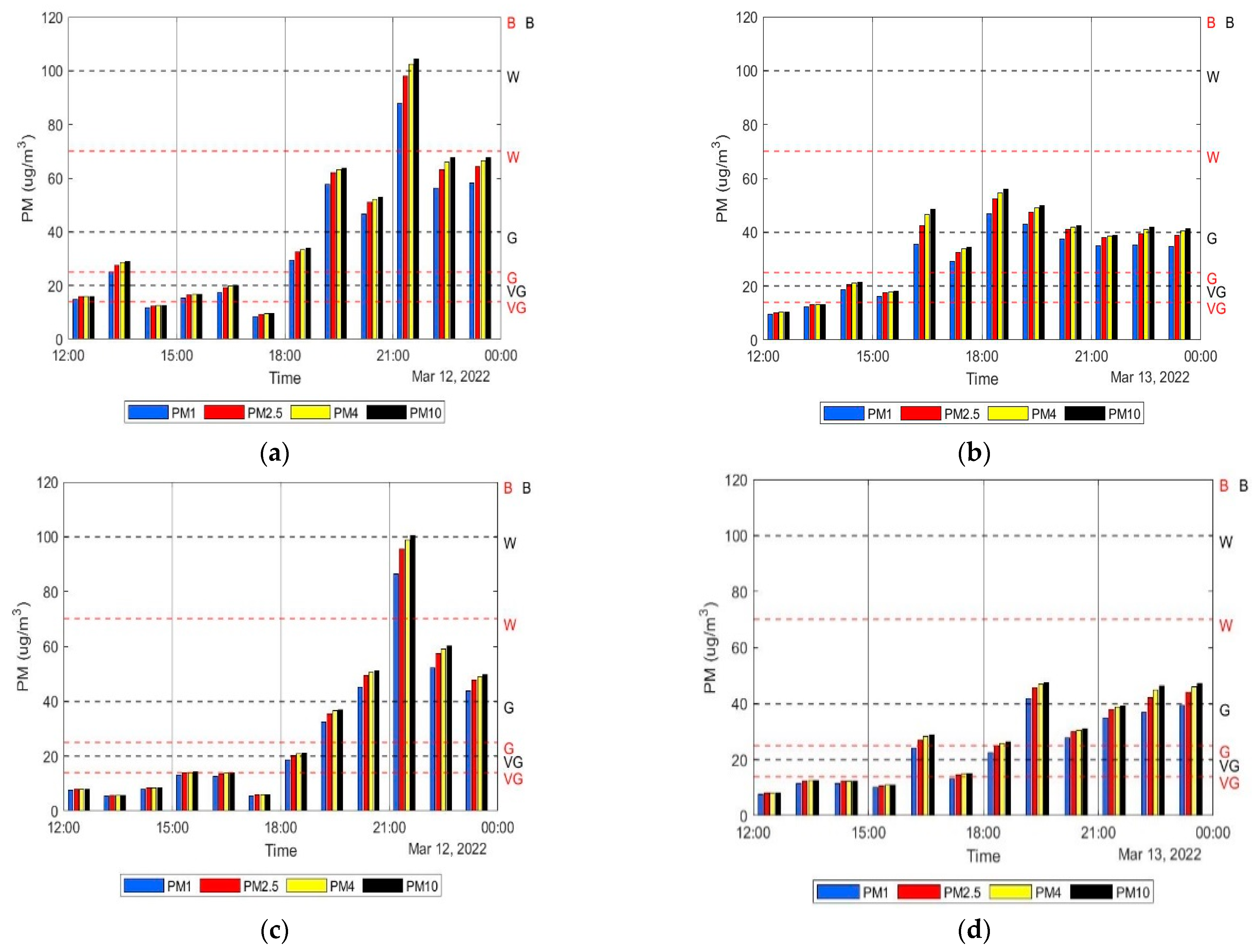
Figure 7 shows the hourly averages of mass concentration of particulate matter. Figure 7a,b were calculated from the measurements that were conducted on the balcony while Figure 7c,d were calculated from the measurements carried out in the garden. If we compare measurements from 12th March, 12:00–24:00, both the measurement on the balcony (Figure 7a) and in the garden (Figure 7c) follow a similar trend. The hourly averages of PM mass concentration tend to be slightly higher for the balcony measurements compared to the garden measurements, especially at 13:00–14:00, 19:00–20:00, 22:00–24:00. It can be seen from Figure 6a that during that time, there were frequent peaks recorded by the sensor S1, but also the baseline PM mass concentration was higher on the balcony than in the garden. As for the measurements from 13th March, 12:00–24:00, the hourly averages of mass concentration of PM also tend to be higher for the balcony measurements (Figure 7b) than the garden measurements (Figure 7c). The biggest difference is at 14:00–15:00, 16:00–19:00. During other measured days the hourly averages of mass concentration are generally higher on the balcony as well. However, there were also a few exceptions when the mass concentration of PM was higher in the garden.

The question which we were interested in next was: how much does the correlation between PM10 and meteorological factors (temperature, humidity, pressure) change with the change in location? The measurements taken showed that even though the two measuring places were distant from each other by 35 m, there was a significant difference between the immediate mass concentration of PM (e.g., short but high peaks in the mass concentration) (Figure 5 and Figure 6) and a slight difference in hourly averages of the mass concentration of PM (Figure 7). This raises the question: how will that affect the correlation?

Table 9. Air Quality Index for the balcony measurement.

Date	PM2.5 * (µg/m3)	IPM2.5	PM10 * (µg/m3)	IPM10
11 March 2022	48.0	132	53	49
12 March 2022	33.1	95	35	32
13 March 2022	33.9	97	37	34
14 March 2022	34.5	98	35	33
15 March 2022	44.9	124	46	43
16 March 2022	71.7	159	74	60
17 March 2022	54.2	147	56	51
18 March 2022	28.1	85	29	27
19 March 2022	44.3	123	46	43
20 March 2022	38.4	108	39	36
21 March 2022	30.5	90	31	28

* 24-h average.

shows daily averages of PM2.5 and PM10 as well as their respective air quality sub-indices for the measurement on the balcony. The air quality reached moderate levels during a total of 5 days (on 12–14, 18 and 21 March), unhealthy for sensitive groups during a total of 5 days (on 11, 15, 17, 19 and 20 March) and unhealthy levels for one day (on 16 March).

As for I_PM2.5 and I_PM10 (

Table 10. Air Quality Index for the garden measurement.

Date	PM2.5 * (µg/m3)	IPM2.5	PM10 * (µg/m3)	IPM10
11 March 2022	27.7	84	30	28
12 March 2022	28.1	85	29	27
13 March 2022	26.6	82	28	26
14 March 2022	32.8	95	34	31
15 March 2022	38.4	108	39	36
16 March 2022	61.1	154	62	55
17 March 2022	54.1	147	55	51
18 March 2022	25.2	79	26	24
19 March 2022	36.3	103	37	35
20 March 2022	32.4	94	33	31
21 March 2022	35.6	101	36	33

* 24-h average.

) for the garden measurement, the air quality was moderate during a total of 6 days (on 11–14, 18 and 20 March), unhealthy for sensitive people during a total of 4 days (on 15, 17, 19 and 21 March) and unhealthy during 1 day (on 16th March). Hourly averages of PM2.5 and PM10 as well as I_PM2.5 and I_PM10 were better in the garden (Table 10) than on the balcony (Table 9) every day except for 21 March 2022. This is another confirmation that the distance from the source of PM (family houses which use wood combustion as a heat source) impacts the air quality.

Next, both measurements were divided into 12-h intervals.

Table 11. Correlation between mass concentration of PM10 and temperature, humidity, pressure: balcony measurement.

Interval	PM10 and Temperature	PM10 and Humidity	PM10 and Pressure
12 March, 0:00–12:00	−0.032 ***	0.058 ***	0.158
12 March, 12:00–24:00	−0.538 **	0.605 **	−0.560 **
13 March, 0:00–12:00	−0.031 ***	0.018 ***	0.061 ***
13 March, 12:00–24:00	−0.276 *	0.273 *	0.192 *
14 March, 0:00–12:00	0.139	−0.089	0.354
14 March, 12:00–24:00	−0.140 *	0.076	0.069
15 March, 0:00–12:00	0.446 *	−0.431 **	0.432
5 March, 12:00–24:00	−0.257	0.262	−0.150
16 March, 0:00–12:00	−0.209	0.480	−0.252
16 March, 12:00–24:00	−0.381	0.257	0.039 ***
17 March, 0:00–12:00	−0.101	0.133	0.213
17 March, 12:00–24:00	−0.061 ***	0.069	0.006 **/***
18 March, 0:00–12:00	−0.120	0.153 *	−0.048 ***
18 March, 12:00–24:00	−0.460	0.452	−0.205
19 March, 0:00–12:00	−0.123	0.129	−0.024 ***
19 March, 12:00–24:00	−0.490	0.518	0.520 **
20 March, 0:00–12:00	−0.135 *	0.202 *	0.003 ***
20 March, 12:00–24:00	−0.534 **	0.502	−0.435

* The values of r which show weak correlation in Table 6 but show moderate correlation in Table 7 or vice versa. ** The values of r which differ from Table 7 by less than 0.05. *** r for which p > α.

and

Table 12. Correlation between mass concentration of PM10 and temperature, humidity, pressure: garden measurement.

Interval	PM10 and Temperature	PM10 and Humidity	PM10 and Pressure
12 March, 0:00–12:00	−0.180	0.185	−0.016 ***
12 March, 12:00–24:00	−0.504 **	0.581 **	−0.599 **
13 March, 0:00–12:00	−0.270	0.219	0.121
13 March, 12:00–24:00	−0.527 *	0.553 *	0.494 *
14 March, 0:00–12:00	0.000 ***	0.007 ***	0.166
14 March, 12:00–24:00	−0.402 *	0.388	0.164
15 March, 0:00–12:00	0.384 *	−0.433 **	0.553
15 March, 12:00–24:00	−0.334	0.398	−0.303
16 March, 0:00–12:00	0.293	0.626	−0.370
16 March, 12:00–24:00	−0.283	0.090	−0.306
17 March, 0:00–12:00	−0.356	0.376	0.031 ***
17 March, 12:00–24:00	−0.190	0.263	0.010 **/***
18 March, 0:00–12:00	−0.329	0.411 *	−0.165
18 March, 12:00–24:00	−0.522	0.538	−0.379
19 March, 0:00–12:00	−0.257	0.304	−0.119
19 March, 12:00–24:00	−0.577	0.658	0.507 **
20 March, 0:00–12:00	−0.405 *	0.492 *	−0.206
20 March, 12:00–24:00	−0.577 **	0.594	−0.543

* The values of r which show moderate correlation in Table 7 but weak correlation in Table 6 or vice versa. ** The values of r which differ from Table 6 by less than 0.05. *** r for which p > α.

consist of the correlation coefficients from the measurement on the balcony and in the garden, respectively. As is the case with Table 5, Table 6 and Table 7, the cells within the table are colored according to how strong the correlation between PM10 and other physical quantities is. If |r| < 0.4, then the cells are white, as there is weak correlation (or no correlation if r approaches 0). If 0.4 < |r| < 0.8, there is moderate correlation, and the cells are shaded light grey. Dark grey is used for cells with |r| > 0.8, or strong correlation [27]. However, in our case, no strong correlation was found in Table 11 and Table 12, so there are no cells shaded with dark grey color. For most intervals, in both Table 11 and Table 12, either weak or no correlation was found. In Table 11, only 15 out of 54 correlation coefficients show moderate correlation. In Table 12, the number of correlation coefficients that correspond to moderate correlation is 21. Seven cells in total change from having none or weak correlation in Table 6 to having moderate correlation in Table 7 and one cell changes from r > 0.4 in Table 11 to r < 0.4 in Table 12 (correlation between mass concentration of PM10 and temperature on 15 March, 0:00–12:00). However, the value of this cell in Table 12 is 0.384, which is close to 0.4. Still in most cases, the correlation improves during the garden measurement (Table 12). There is even one interval, in which all correlations (between PM10 and temperature, PM10 and humidity, as well as PM10 and pressure) improve from weak correlation in Table 11 to strong correlation in Table 12—13 March, 12:00–24:00. Mass concentration of PM10 during this interval can be seen in Figure 6b (both the balcony and the garden measurement) and the hourly averages of mass concentration of PM is shown in Figure 7b (the balcony measurement) and Figure 7d (the garden measurement). The cells, which have moderate correlation in Table 11 and weak correlation in Table 12 and vice versa, are marked by one asterisk (*).

Although there are many cases where correlation coefficient changes from Table 11 to Table 12, there are also some intervals, in which the changes are very small. Cells, in which the difference between r in Table 11 and Table 12 is smaller than 0.05, are marked with a double asterisk (**). There are eight such cells, three of which belong to the same interval (12 March, 12:00–24:00). The mass concentration of PM10 for this interval is shown in Figure 6a and the hourly averages in Figure 7a,c. The comparison of PM10 mass concentration and meteorological factors for those intervals is shown in Figure 8 and Figure 9.

The fact that most correlation coefficients indicate either weak or no correlation, and some indicate only moderate correlation (Table 11 and Table 12), while the previous measurements in Košice showed the majority of intervals as having moderate correlation with some strong correlation or weak correlation, may be caused by the peaks that have been measured in the village. After all, even the garden measurements, which show smaller peaks that are less frequent, improve the correlation slightly. In Košice no peaks were measured and therefore mass concentration of PM is distributed more evenly even during a longer time interval. This even distribution is disrupted in the village by residents in family houses burning wood and therefore creating these local non-regular short increases in particulate matter. These peaks then affect the correlation found in Table 6 and Table 7.

As for the p-values corresponding to r in Table 11 and Table 12, there were eleven p-values (two-tailed, n = 8640) which exceeded α (as corresponding to Table 3) in Table 11, and only five p-values which exceeded α in Table 12. For the rest of the intervals, p ≤ α. This suggests that the peaks, which are more often found in the balcony measurement (Table 11), negatively impact the correlation between PM and meteorological factors.

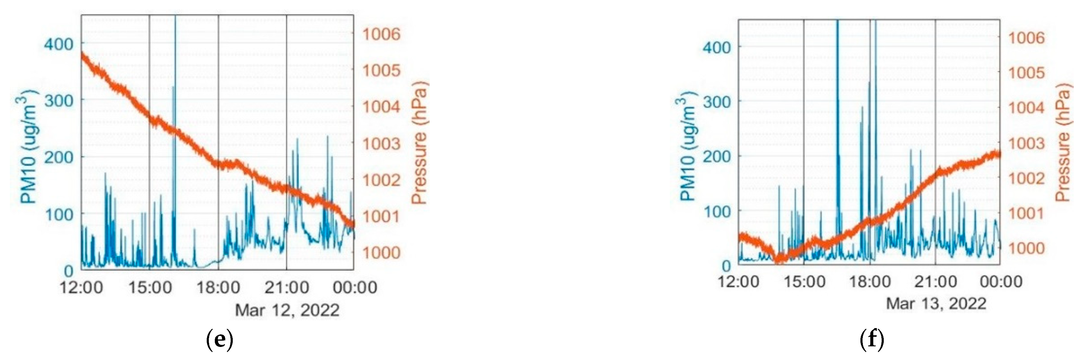
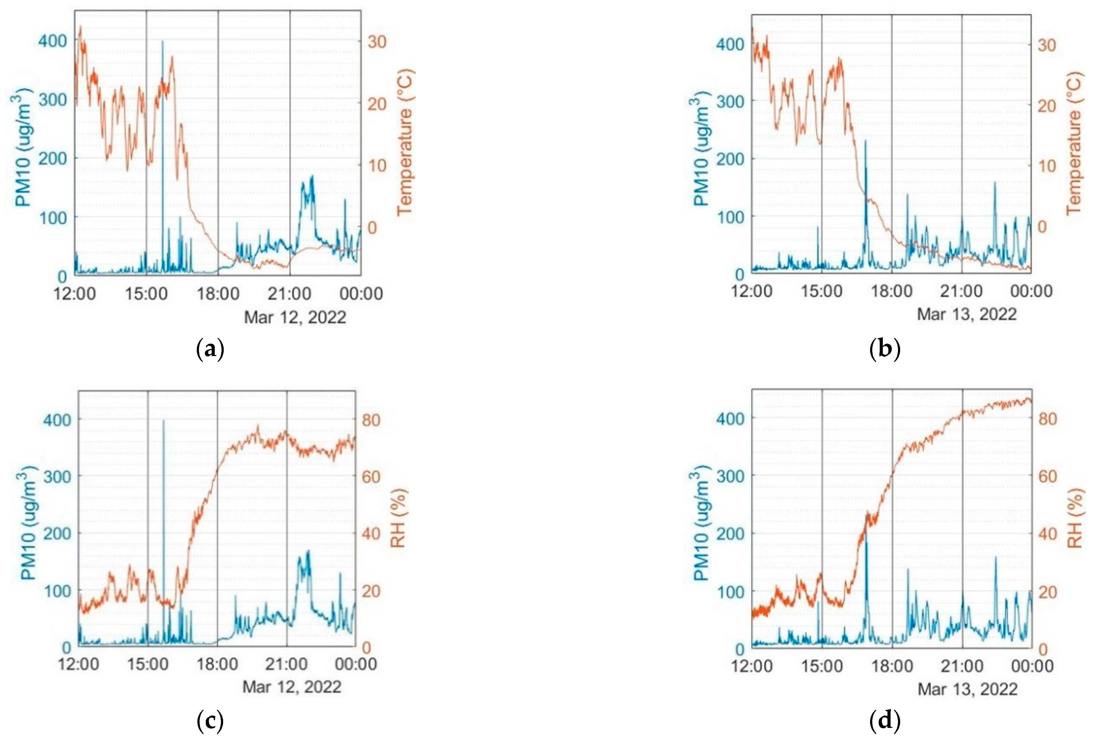
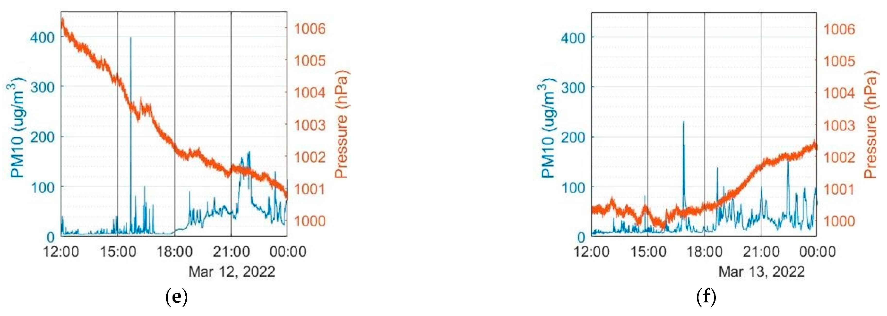
To better illustrate correlation, the changes in PM10 mass concentration and temperature, humidity, and pressure during the intervals mentioned above (12 and 13 March, 12:00–24:00) are shown in Figure 8 (balcony measurement) and Figure 9 (garden measurement). In Figure 8b,d,f, three peaks of PM10 mass concentration exceed the y-axis scale, just like in Figure 6b. They reach 477.37, 760.45 and 508.15 µg/m³. The effect the peaks have on the correlation can be best seen in Figure 8b, where PM10 mass concentration and temperature are plotted. Even in the section where temperature is constant or decreasing slowly (18:00–24:00), there is still a number of changes in PM10 caused by the peaks. Therefore, it is reasonable that weak correlation was found in those intervals.

Now compare the changes in PM10 mass concentration in Figure 8b to the changes in PM10 mass concentration in Figure 9b. The peaks are smaller, but, more importantly, less frequent, and therefore the distribution of mass concentration is more uniform. There are still some peaks, and there are not many clear examples when both quantities simultaneously increase or decrease, or where one quantity increases and the other quantity decreases (compared to Figure 4, when such intervals can be clearly identified). As such, from the graph in Figure 9b, it is more difficult to predict whether there will be any correlation found. However, we can rely on the correlation coefficient to reveal if there is any correlation between the measured quantities and how strong it is (ex., for Figure 9b). Moderate correlation was found between PM10 mass concentration and temperature. Other graphs in Figure 8 and Figure 9 can be compared in a similar way.

4. Discussion

Comparing our measurements in Košice at DTIEE with our measurements in a small village, we have found that in a small village, short-term (over the course of several seconds to minutes) increases in PM mass concentrations were very common due to the measuring place being located near the sources of PM (houses heating with solid fuel). In Košice at DTIEE, the levels of mass concentration were much more stable. The increases in mass concentration were more likely to be long term (for example over the course of four days, as demonstrated in this paper). Furthermore, air quality was usually worse in the small village with the exception of the four-day increase in PM mass concentrations in Košice at DTIEE. In fact, the air quality on 29 January 2022 is much more indicative of the usual air quality in Košice, which we concluded in our previous research [22]. Furthermore, air quality sub-indices calculated from PM2.5 and PM10 indicate that PM2.5 affects the air quality to a greater degree, regardless of the place of measurement. I_PM2.5 was consistently higher that I_PM10 both in Košice at DTIEE and in the small village (on the balcony and in the garden).

We also paid attention to comparing the measurements in a small village on the balcony vs. in the garden. The measuring place on the first floor balcony was closer to the sources of PM (chimneys of the houses, which used solid fuel/wood for heating) by about 35 m than the measuring place in the garden. It was found that the peaks (short-term increases in PM mass concentration) recorded in the garden were lower and less frequent than those recorded on the balcony at the same time.

As for the correlation between PM and meteorological factors (temperature, humidity, barometric pressure), more cases of correlation were found in Košice than when measuring in a small village. This may be due to a more even distribution of PM within Košice, as the main source of PM in Košice (road transport) is more evenly distributed within the city (although the US Steel factory distant by 12 km from the department where the measurements were carried out must also be taken into account). Therefore, PM is more homogeneously distributed in Košice than in a small village, where the chimneys of houses are located relatively near each other and pollute the air with smoke from wood combustion. Therefore it seems that, especially during the heating season (fall/winter/spring), the air quality is better in a big city like Košice than in a small village, where it is even possible to feel the deteriorating air quality during the heating season with one’s own senses. As fine particles (PM2.5) have a significant negative impact on the health of children and the elderly, the need to measure PM concentrations has become greater than before. The fact that the typical particle size is in the range of 0.5–0.75 μm (these particles are included in PM1, and the sensor is able to measure particles with a diameter larger than 0.3 μm) makes the situation with the air we breathe even more alarming, as the ultrafine particles (PM0.5) very easily penetrate into the human bloodstream.

Overall, when the correlation was found, the measured PM10 had a tendency to correlate negatively with temperature and pressure and positively with humidity, which proves some of the statements in [12,13,14,15]. A sudden change in the correlation over 12 h from a strong/moderate correlation to weak correlation (Table 2, first and second lines) suggests that another factor, which might affect the measurement, may be the wind, as it has been stated by [12,13]. Just like the wind, another group of houses, which are closer to the garden, may affect the measurements in the garden but not on the balcony. The impact of wind on PM concentration and correlation will be assessed in the near future. Regional differences, as concluded by study [16] may also be a factor as to why the strength of the correlation varies with measuring location (city vs. village). With the current crisis in Europe and the rising prices of gas and electricity, as well as regionally available wood for heating family homes, we can assume a worsening of the AQI index and, later, even greater health problems for the population.

References

1. Hester, R.E. Airborne Particulate Matter: Sources, Atmospheric Processes and Health; Royal Society of Chemistry: Cambridge, UK, 2016. [Google Scholar]
2. Kremler, M. Report on Air Quality in Slovak Republic in 2020; Slovak Hydrometeorological Institute: Bratislava, Slovakia, 2020. (In Slovak) [Google Scholar]
3. Schraufnagel, D.E. The Health Effects of Ultrafine Particles. Exp. Mol. Med. 2020, 52, 311–317. [Google Scholar] [CrossRef] [PubMed]
4. World Health Organization. Health Effects of Particulate Matter: Policy Implications for Countries in Eastern Europe, Caucasus and Central Asia. J. Korean Med. Assoc. 2013, 50, 3. [Google Scholar]
5. Kampa, M.; Castanas, E. Human Health Effects of Air Pollution. Environ. Pollut. 2008, 151, 362–367. [Google Scholar] [CrossRef] [PubMed]
6. Kyung, S.Y.; Jeong, S.H. Particulate-Matter Related Respiratory Diseases. Tuberc. Respir. Dis. 2020, 83, 116–121. [Google Scholar] [CrossRef] [PubMed]
7. Götschi, T.; Heinrich, J.; Sunyer, J.; Künzli, N. Long-Term Effects of Ambient Air Pollution on Lung Function: A Review. Epidemiology 2008, 19, 690–701. [Google Scholar] [CrossRef] [PubMed] [Green Version]
8. Brook, R.D. Cardiovascular Effects of Air Pollution. Clin. Sci. 2008, 115, 175–187. [Google Scholar] [CrossRef] [PubMed] [Green Version]
9. World Health Organization. Ambient (Outdoor) Air Pollution. Available online: https://www.who.int/news-room/fact-sheets/detail/ambient-(outdoor)-air-quality-and-health (accessed on 30 May 2022).
10. Mühlfeld, C.; Rothen-Rutishauser, B.; Blank, F.; Vanhecke, D.; Ochs, M.; Gehr, P. Interactions of Nanoparticles with Pulmonary Structures and Cellular Responses. Am. J. Physiol. Lung Cell. Mol. Physiol. 2008, 294, L817–L829. [Google Scholar] [CrossRef] [PubMed] [Green Version]
11. Liu, Y.; Zhou, Y.; Lu, J. Exploring the Relationship between Air Pollution and Meteorological Conditions in China under Environmental Governance. Sci. Rep. 2020, 10, 14518. [Google Scholar] [CrossRef] [PubMed]
12. Jiang, B.; Sun, C.; Mu, S.; Zhao, Z.; Chen, Y.; Lin, Y.; Qiu, L.; Gao, T. Differences in Airborne Particulate Matter Concentration in Urban Green Spaces with Different Spatial Structures in Xi’an, China. Forests 2022, 13, 14. [Google Scholar] [CrossRef]
13. Yang, H.; Peng, Q.; Zhou, J.; Song, G.; Gong, X. The Unidirectional Causality Influence of Factors on PM2.5 in Shenyang City of China. Sci. Rep. 2020, 10, 8403. [Google Scholar] [CrossRef] [PubMed]
14. Kim, M.J. Changes in the Relationship between Particulate Matter and Surface Temperature in Seoul from 2002–2017. Atmosphere 2019, 10, 238. [Google Scholar] [CrossRef] [Green Version]
15. Luo, H.; Zhou, W.; Jiskani, I.M.; Wang, Z. Analyzing Characteristics of Particulate Matter Pollution in Open-Pit Coal Mines: Implications for Green Mining. Energies 2021, 14, 2680. [Google Scholar] [CrossRef]
16. Tai, A.P.K.; Mickley, L.J.; Jacob, D.J. Correlations between Fine Particulate Matter (PM2.5) and Meteorological Variables in the United States: Implications for the Sensitivity of PM2.5 to Climate Change. Atmos. Environ. 2010, 44, 3976–3984. [Google Scholar] [CrossRef]
17. Štrbová, K.; Raclavská, H.; Bílek, J. Impact of Fugitive Sources and Meteorological Parameters on Vertical Distribution of Particulate Matter over the Industrial Agglomeration. J. Environ. Manag. 2017, 203, 1190–1198. [Google Scholar] [CrossRef] [PubMed]
18. Sensirion. Particulate Matter Sensor for Air Quality Monitoring and Control. Datasheet SPS30. Available online: https://cdn.sos.sk/productdata/98/89/92718144/sps30-2.pdf (accessed on 30 May 2022).
19. Sensirion. Automotive Grade Humidity and Temperature Sensor. Datasheet SHT3x-DIS. Available online: https://www.mouser.com/datasheet/2/682/Sensirion_Humidity_Sensors_SHT3x_Datasheet_digital-971521.pdf (accessed on 30 May 2022).
20. TE Connectivity. Barometric Pressure Sensor, with Stainless Steel Cap. MS5611-01BA03 Datasheet. Available online: https://www.te.com/commerce/DocumentDelivery/DDEController?Action=showdoc&DocId=Data+Sheet%7FMS5611-01BA03%7FB3%7Fpdf%7FEnglish%7FENG_DS_MS5611-01BA03_B3.pdf%7FCAT-BLPS0036 (accessed on 30 May 2022).
21. BOSCH. Digital Pressure Sensor. BMP280 Datasheet. Available online: https://cdn-shop.adafruit.com/datasheets/BST-BMP280-DS001-11.pdf (accessed on 30 May 2022).
22. Kirešová, S.; Guzan, M.; Galajda, P. Measuring Particulate Matter (PM) using SPS30. In 32nd International Conference Radioelektronika; IEEE: Košice, Slovakia, 2022; pp. 160–165. [Google Scholar]
23. Shihab, A.S. Assessment of Ambient Air Quality of Mosul City/Iraq Via Air Quality Index. J. Ecol. Eng. 2021, 22, 241–250. [Google Scholar] [CrossRef]
24. United States Environmental Protection Agency. Technical Assistance Document for the Reporting of Daily Air Quality—The Air Quality Index (AQI). Available online: https://www.airnow.gov/sites/default/files/2020-05/aqi-technical-assistance-document-sept2018.pdf (accessed on 14 July 2022).
25. Naaman, M. Almost Sure Hypothesis Testing and a Resolution of the Jeffreys-Lindley Paradox. Electron. J. Stat. 2016, 10, 1526–1550. [Google Scholar] [CrossRef]
26. Slovak Hydrometeorological Institute. Hourly Concentrations of Air Pollutants. Available online: https://shmu.sk/sk/?page=1&id=oko_imis (accessed on 4 February 2022). (In Slovak).
27. Hanák, R. Correlation. Available online: https://statistikapspp.sk/korelacia/ (accessed on 1 June 2022). (In Slovak).
Figure 1. Comparative measurement between two SPS30 sensors: (a) Sensor 1 (S1); (b) Sensor 2 (S2); (c) Difference between Sensor 1 and Sensor 2 (S1–S2); (d) scatter plot of the difference between Sensor 1 and Sensor 2 (S1–S2).
Eng 03 00025 g001
Figure 2. Measurements carried out by eight BMP280 sensors: (a) temperature; (b) pressure.
Eng 03 00025 g002
Figure 3. Hourly averages of mass concentration of PM1, PM2.5, PM4, PM10 measured in January 2022 in Košice at DTIEE: (a) 25th 12:00–24:00; (b) 26th 0:00–12:00; (c) 26th 12:00–24:00; (d) 27th 0:00–12:00; (e) 27th 12:00–24:00; (f) 28th 0:00–12:00; (g) 28th 12:00–24:00; (h) 29th 0:00–12:00. Dashed lines represent limit values for the air quality with respect to concentration of PM2.5 (red) or PM10 (black). Abbreviations next to the dashed lines indicate the air quality: VG = Very Good, G = Good, W = Worsened, B = Bad, corresponding to Table 4.
Eng 03 00025 g003
Figure 4. Changes in the measured quantities: PM10 and Temperature in January 2022 (a) 25th 12:00–24:00; (b) 26th 0:00–12:00; PM10 and Humidity on (c) 25th 12:00–24:00; (d) 26th 0:00–12:00; PM10 and Pressure on (e) 25th 12:00–24:00; (f) 26th 0:00–12:00.
Eng 03 00025 g004
Figure 5. Measurement of PM10 in a small village on the balcony of the family house (blue line) and in the garden (red line).
Eng 03 00025 g005
Figure 6. Measurement of PM10 on the balcony (blue line) and in the garden (red line) in March 2022: (a) 12th 12:00–24:00; (b) 13th 12:00–24:00.
Eng 03 00025 g006
Figure 7. Hourly averages of mass concentration of PM1, PM2.5, PM4, PM10: measured on the balcony in March 2022: (a) 12th 12:00–24:00, (b) 13th 12:00–24:00; measured in the garden on: (c) 12th 12:00–24:00, (d) 13th 12:00–24:00. Abbreviations next to the dashed lines indicate the air quality: VG = Very Good, G = Good, W = Worsened, B = Bad, corresponding to Table 4.
Eng 03 00025 g007
Figure 8. Changes in the measured quantities: PM10 and temperature (a) on 12 March 2022, (b) 13 March 2022; PM10 and humidity (c) on 12 March 2022, (d) on 13 March 2022, PM10 and pressure (e) on 12 March 2022 and (f) 13 March 2022; measured on the balcony.
Eng 03 00025 g008aEng 03 00025 g008b
Figure 9. Changes in the measured quantities: PM10 and temperature (a) on 12 March 2022, (b) 13 March 2022; PM10 and humidity (c) on 12 March 2022, (d) on 13 March 2022, PM10 and pressure (e) on 12 March 2022 and (f) 13 March 2022; measured in the garden.
Eng 03 00025 g009aEng 03 00025 g009b