Homogenization Method to Calculate the Stiffness Matrix of Laminated Composites

Abstract

New analytical models have been developed for predicting equivalent Young’s and shear moduli of laminate composites. Sets of procedures and calculations are presented in order to obtain equivalent properties in all levels, lamina and laminate. An ultimate path to predict the mechanical properties of laminated composites on the perspective of the material, orientation, and thickness has been developed. By calculating the mechanical properties using Chamis model then an Objectif function with five norms, these norms allow the mechanical properties to be examined and the ultimate answer to be predicted. Another model discusses an alternative concept of equivalent lamina elements (ELEs) by first using Chamis model for hybrid composites. Next, the ELEs are laminated in the direction and integrated into the compliance matrix for each ply. In addition, four new Generalization models for equivalence in thickness and in angle are presented in this paper. The analytical results are validated against other developed models in published articles as well as experimental results. Numerical case studies were conducted to assess the precision of results from the suggested models. The results demonstrated the capability and efficiency of the presented models for predicting the mechanical properties of multi-layer/multi-material laminate composites under different orientation conditions.

1. Introduction

Composite materials consist of two or more components such as fiber and matrix and may or may not be fillers in case of polymer composite materials. They have a wide range of applications, such as industrial, automotive engineering medical aerospace electrical, transportation, and sports [1].

The integration of two materials gives better properties compared with individual components [2].

Composites structures are often classified as four basic structures or levels, i.e., lamina, laminate, sandwich, and woven composites. A lamina (also called a ply or layer) is a single flat layer of unidirectional fibers or woven fibers arranged in a matrix, a thin layer of a composite material, while a laminate is a stack of plies of composites. Each layer can be laid at various orientations and can be made up of different material systems.

In recent years, conventional materials are continuously being replaced by a variety of composite materials. This fact has caused an increasing interest on the modeling of composites. Several approaches have been developed, but there is still a strong need of predicting models that can be used for the stiffness and strength assessment of this type of materials in practical situations. [1] Constitutive models for fiber-reinforced composite laminates can be classified according to the scale in which they are defined [3].

1.1. Problematic

In composite materials, the properties are different depending on the fiber orientation in the matrix, so knowing the properties or obtaining the correct and more accurate properties is a very important key when it comes to analyzing the structures [4]. Using composite materials in engineering industries requires complicated analysis and modeling which in most cases computer software runs. It is difficult and time-consuming to calculate the properties of a very thick laminate with each layer having different stacking sequences. It would be simpler and less time-consuming to use average properties that would represent the desired model, instead of going through calculations and obtaining stiffness matrices for each layer, i.e., ply-by-ply approach.

While experimental tests made to determine the effective elastic properties of composites, i.e., Young’s and shear moduli (Ex, Ey, Ez, Gxy, Gxz, and Gyz) and Poisson’s ratios (νxy, νxz, and νyz), are expensive in terms of money and time, analytical and numerical modeling could present a good alternative solution for industries and the obtained results are supposed to be more accurate. These methods have the disadvantages of a great deal of time consumed on the tasks of defining the geometry of the composite, meshing, and calculation procedures, besides the need of super computers to make the computation. Analytical modeling presents a more flexible and easier tool in terms of geometric modeling and the time saved in calculation, without the need of super computers. Therefore, in order to overcome these difficulties, equivalent properties of lamina or laminate are often used. Equivalent properties or effective stiffness properties are an average measure of the stiffness of the desired material. The actual averaging process must be done carefully and delicately in order to obtain equivalent properties.

Up to now, many models have been proposed to analyze the microstructures and mechanical performance of laminates composites. Many scholars have paid great efforts to the prediction of mechanical properties of laminate composite, but there is no physical model or method that can predict the mechanical properties and behavior of the composite materials with different sets of parameters in terms of orientation, material properties, and thicknesses. The novelty of this paper is to provide the most accurate results of the mechanical properties using an effective algorithm that can be used as an alternative to software or experimental studies. Different analytical models predict different elastic properties of composites. Additional problems involve estimating model adequacy and choosing the most accurate model. Different models are more accurate, depending on the composite content, the shape of the inclusions, and the relationship between the properties of the inclusions and the matrix [2].

The works on the mechanical analysis and optimization design of laminate composites are extremely limited. To the author’s knowledge, there is no literature on applying the classical laminate theory to analyze the mechanical properties of laminate composites. In addition, there is no literature on using the ABD matrix (The ABD matrix is a 6 × 6 matrix that serves as a connection between the applied loads and the associated strains in the laminate. It essentially defines the elastic properties of the entire laminate) to find and predict the mechanical/engineering properties of laminated composites, such as compliance or stiffness matrices. Therefore, it is valuable to propose a theoretically analytical model to investigate the mechanical properties of laminate composites due to its advantages in low modeling cost and high computational efficiency.

It is important to calculate strain and stress to know the effectiveness of compound combinations. Combined applications are widely available in the field of automotive, airports, and sports.

1.2. State of Art

There have been a number of publications regarding predicting composite materials properties and equivalent or effective properties of composite materials. Richardson [5] predicted stiffness using rule of mixtures (ROM), ROM with efficiency factors, classical laminate analysis, and empirical formulas. To discuss effective properties of composites, Lydzba [6] used the homogenization method to define the heterogeneous medium that possesses the property of statistical homogeneity as an equivalent homogeneous material that would have the same average properties. Chan [7] represented the lumping procedures, in which a group of plies lumps into a single layer to reduce the size of the problem and to increase the efficient computation, which is often used in thick composite structure modelling. On the other hand, Kumar [8] presented a new analytical model to replace the original laminate ABD by much simpler ABD-equivalent virtual material models. These virtual material models, under the usual assumptions made in the lamination theory, have the same constitutive relationship as the corresponding two-dimensional (2D) plate model of the original laminate but require only a small fraction of computational integration costs in three dimensions.

It is noted that all the numerical approaches consist in building a representative volume element (RVE) able to statistically represent the overall material [9]. Prescribed loads or displacements are applied at the RVE, and the resulting stresses and strains are correlated with the whole structure at the macroscale by means of the averaging principle [10]. However, 2D RVEs may not give accurate results for composite materials [5], especially for out-of-plane properties, demanding more laborious and time-consuming three-dimensional (3D) models [6]. As an alternative, analytical models are used for composite homogenization, usually being derived from the strength of materials or semi-empirical relations. Numerical and analytical models usually share important assumptions in the homogenization process, namely neglecting the fiber/matrix interface and, homogeneous fibers and matrixes and perfect fiber alignment [9]. In addition, in the evaluation process, the properties of the individual constituents are required, and these may be hard to obtain, especially for fibers [9].

Regarding the longitudinal Young’s modulus (E1) and the in-plane Poisson ratio (ν12), the ROM is able to provide accurate results, even for hybrid composites [7,8,9,10,11]. For the other engineering constants, Banerjee [7] extended the semi-empirical models proposed by Halpin [12].

Alternatively, as proposed by Chamis [13], HC (Hybrid Composite) properties can be estimated by splitting it on the primary composite (PC) and the secondary composite (SC), where the first is reinforced by fiber 1 and the second is reinforced by fiber2, with the matrix proportionally distributed. The PC and SC properties are calculated analogously to single-fiber composites [8]. Then, the ROM is applied to compute E2 from PC and SC. This same methodology is adopted by Chamis to compute G12 and G23. ν23 can be computed under the transversally isotropic consideration [9].

The model presented by Chou [11] applies the same division and equations proposed by Chamis [8] to compute PC and SC properties. However, the final properties are evaluated using an inverse ROM.

The relations presented above are well accepted in the literature for laminate composites [14]. However, many new models with greater complexity were developed, avoiding assumptions related to long fibers [15] and straight fibers [16] or focusing on other reinforcement geometries, such as particles or nanotubes [17]. The semi-analytical model proposed by Aboudi [18] was also applied for HC [19], yielding good mechanical predictions. The tensile loadings of specimens produce different failure types, and researchers have studied the inhomogeneity of the matrix [20]. Research interest has been focused on towards fiber-reinforced polymeric composites, as these composite materials exhibit excellent mechanical properties. Parvanesh et al. [21] studied the mechanical behavior of PVC (poly(vinyl chloride)) nanocomposites. They have studied the Young’s modulus and tensile strength of polymer composites, and the result suggested that good stress transfer can be obtained at an amorphous interface, depending on the polymer.

The local/global stiffness matrix approach is similar to the transfer and flexibility matrix formulation presented by Bufler [22] for isotropic layered media with constant elastic properties. This approach was later reformulated in terms of the local stiffness matrix by Rowe and Booker [23] and applied to nonhomogeneous isotropic layered soils. Chatterjee et al. [24] extended the method to anisotropic layered media for generalized plane deformation problems and used it to solve the problem of an interlaminar crack in an arbitrarily laminated composite plate under three-point loading.

1.3. Paper Organization

The first section introduces basic ideas about composites including fibers and matrices and basic definitions used in the mechanics of composites. This section starts with a review of basic topics of stress, strain, and elastic moduli. Then, the mechanical behaviors of a single lamina were discussed, including concepts about the stress–strain relationship for a lamina and the stiffness and strength of a lamina, and finally, the equivalence in orientation was discussed by studying the case of rotating fibers and rotating the whole ply, i.e., fiber and matrix in a laminate composite.

Secondly, two ways to find the equivalence in thickness were presented using the greatest common divisor (GCD) and another mathematical method based on the stress- strain relation and Hook’s Law.

Thirdly, two new analytical models were developed for predicting equivalent Young’s and Shear moduli of a laminate composite. The mechanical properties was calculated using Chamis model and an Objectif function with five norms, which allowed the mechanical properties to be examined and ultimate answer to be predicted. Moreover, another model, an alternative concept of equivalent lamina elements (ELEs), was first established using Chamis model for hybrid composites. Next, the ELEs were laminated in the direction and integrated into the compliance matrix for each ply. Finally, the results obtained with these models were compared to experimental results from other papers and journals, and some conclusions are shown.

The objective of the paper is to present new analytical models for analyzing the mechanical properties of laminate composites in all levels, i.e., lamina, laminate, and structure, from the perspectives of the material, orientation, and thickness. The contribution of all unit cells to the elastic properties of specimen was considered in the analytical model. In addition, the effects of the fiber orientation and thickness on the elastic properties were discussed in detail. Finally, some valuable conclusions are drawn.

An efficient recursive algorithm, the stiffness matrix method, has been developed for generally anisotropic multi-layered media. This algorithm has the computational efficiency and simplicity of the standard transfer matrix method and is unconditionally computationally stable for high frequency and layer thickness. In this algorithm, the stiffness (compliance) matrix is calculated for each layer and recursively applied to generate a stiffness (compliance) matrix for a layered system.

This algorithm allows researchers and end users to calculate the stiffness and compliance matrix of any composite material, with any form, orientation, or thickness, by saving time and cost while finding the optimal solution.

2. Methodology

In this paper, we calculated the mechanical properties of laminate composites on three different levels and on three different categories. In one category, the variety of materials used and their homogenization that consisted of two different methods were discussed. In the other categories or paths, a variety of thicknesses and orientation, in which we are able to provide researchers the ultimate path and algorithm to calculate the stiffness matrix of laminated composites and to predict the mechanical properties, was discussed.

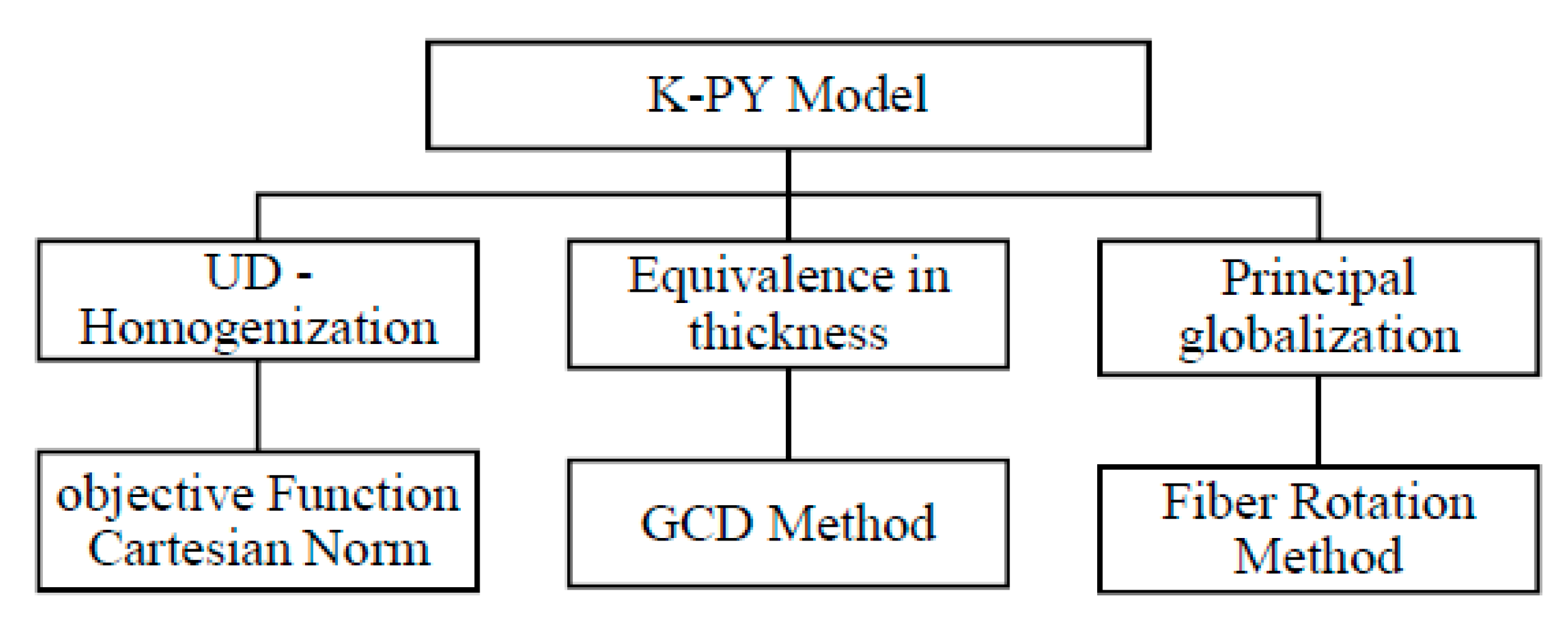
The ultimate path is called the K-PY algorithm, and it is shown in the conclusion part and based on the results found from comparing with experimental data from the literature (Figure 1).

2.1. UD (Unidirectional)—Homogenization:

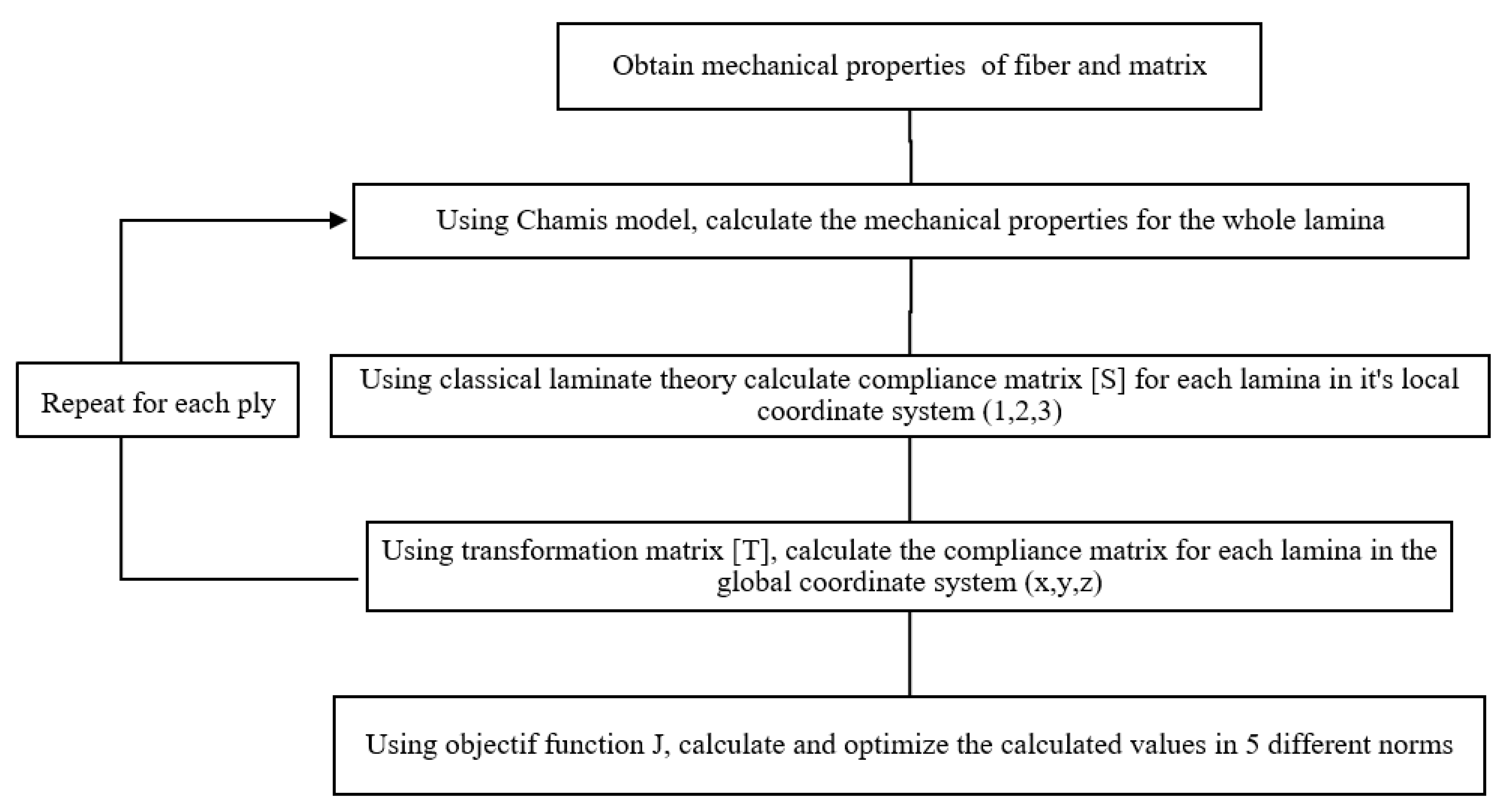
Two new analytical models were proposed to predict the mechanical performance of laminate composites based on Chamis model [25]. The multi-scale modeling strategy was adopted to predict the elastic properties of the composites (Figure 2). The KY analytical model consists totally of three basic steps. Firstly, the elastic performance of constituent components in lamina (or layer), i.e., the fiber and the pure resin matrix, is computed. Secondly, the stiffness matrix of each layer can be obtained by the stiffness-volume-averaging theory. Thirdly, an objective function is implemented to optimize the calculation and to find the optimal solution. Another model was investigated, which consists of finding equivalence of fibers in angle to be in the same direction 0° and to adopt the new fibers into Chamis and Sinclair’s hybrid method [8].

2.1.1. Algorithm Objectif Function

For laminate composites, every kind of unit cell actually includes two types of constituent components, i.e., the fiber and the pure resin matrix. First, the compliance matrix of the lamina was calculated. Similar to many micro-mechanical models, the fibers and the resin matrix assume transversely isotropic, and both of them assume to be linearly elastic in the model. To obtain the elastic properties of the laminate composites, the fiber–matrix ROM proposed by Chamis was chosen to compute the engineering elastic constants. The Chamis micro-mechanical model is the most widely used and trusted model, which gives an equation for all five independent elastic properties as follows [25]:

E₁₁ = V^fE^f₁₁ + V^mE^m,

(1)

E₂₂ = E₃₃ = E^m/(1− √V^f (1 − E^m/(E^f₂₂))),

(2)

G₂₃ = G^m/(1 − √V^f (1 − G^m/(G^f₂₃))),

(3)

G₁₂ = G₁₃ = G^m/(1 − √V^f (1 − G^m/(G^f₂₂))),

(4)

ν₂₃ = V^fν^f₂₃ + V^m (2ν^m − ν₁₂·(E₂₂/E₁₁)),

(5)

ν₁₂ = ν₁₃ = ν^m + ν^f (ν^f₁₂ − ν^m),

(6)

where V^f is the fiber volume fraction; E^f₁₁ is the Young’s elastic modulus of the fiber in principle axis 1; E^f₂₂ is the Young’s elastic modulus of the fiber in principle axis 2; G^f₁₂ is the longitudinal shear modulus of the fiber; G^f₂₃ is the transverse shear modulus of the fiber; ν^f₁₂ is the primary Poisson’s ratio of the fiber; E^m, ν^m, and G^m represent the Young’s elastic modulus, Poisson’s ratio, and shear modulus of the matrix, respectively.

The compliance matrix of the fiber [S] can be calculated easily. For the pure resin matrix pocket, it is generally regarded as isotropic materials. Once the elastic modulus and Poisson’s ratio of the resin matrix are given, it is easy to determine its constitutive relationship.

It is easy to obtain their stiffness matrix in the local material coordinate systems (1, 2, 3) to (x, y, z) by inverting their compliance matrix [Sij] [7].

Then, we can obtain the stiffness in the global coordinate system by transforming the stresses and strains via the generalized transformation matrix as the following form:

$$\left[S\right]={{\left[T\right]}_{\mathrm{k}}}^{\mathrm{T}}{\left[S\right]}_{\mathrm{k}}{\left[T\right]}_{\mathrm{k}}$$

(7)

where l_i, m_i, and n_i (i = 1, 2, 3) are the direction cosines and are defined as the cosines of the angle between the axes of the local and global coordinate systems before and after rotation:

$$\left[T\right]=\left[\begin{array}{cccccc}{l}_1^2& m_1^2& n_1^2& 2m_1{n}_1& 2n_1{l}_1& 2l_1{m}_1\\ l_2^2& m_2^2& n_2^2& 2m_2{n}_2& 2n_2{l}_2& 2l_2{m}_2\\ l_3^2& m_3^2& n_3^2& 2m_3{n}_3& 2n_3{l}_3& 2l_3{m}_3\\ l_2{l}_3& m_2{m}_3& n_2{n}_3& m_2{n}_3+m_3{n}_2& n_2{l}_3+n_3{l}_2& l_2{m}_3+l_3{m}_2\\ l_3{l}_1& m_3{m}_1& n_3{n}_1& m_3{n}_1+m_1{n}_3& n_3{l}_1+n_1{l}_3& l_3{m}_1+l_1{m}_3\\ l_1{l}_2& m_1{m}_2& n_1{n}_2& m_1{n}_2+m_2{n}_1& n_1{l}_2+n_2{l}_1& l_1{m}_2+l_2{m}_1\end{array}\right]$$

(8)

$$\left[\begin{array}{ccc}{l}_1& m_1& n_1\\ l_2& m_2& n_2\\ l_3& m_3& n_3\end{array}\right]=\left[\begin{array}{ccc}sin\tau cos\phi & -sin\phi & -cos\tau cos\phi \\ sin\tau sin\phi & cos\phi & -cos\tau sin\phi \\ cos\tau & 0& sin\tau \end{array}\right]$$

(9)

Each of the matrices is evaluated in ply k, and then the contributions of all the plies n are added.

• Objective function

The objective function indicates how much each variable contributes to the mechanical properties to be optimized. It takes the following general form:

$$\begin{array}{c}\mathrm{J}={\sum }_{i=1}^n[{\left(E_{11}-Ex{x}_{\mathrm{i}}\right)}^n+{\left(E_{22}-Ey{y}_{\mathrm{i}}\right)}^n+{\left(E_{33}-Ez{z}_{\mathrm{i}}\right)}^n+{\left(G_{13}-Gx{z}_{\mathrm{i}}\right)}^n+\\ {\left(G_{23}-Gy{z}_{\mathrm{i}}\right)}^n+{\left(G_{12}-Gx{y}_{\mathrm{i}}\right)}^n+{\left(v_{12}-vxy\right)}^n+{\left(v_{23}-vyz\right)}^n+{\left(v_{13}-vxz\right)}^n],\end{array}$$

(10)

where n is the power of the decision variable Xi; Exx_i, Eyy_i … are the reel values of the mechanical properties; E₁₁, E₂₂ … are the unknown values to be optimized. To solve and optimize the solutions from the Objectif function J, the partial derivative to each component is applied as following:

$$\begin{array}{c}\frac{\partial J}{\partial E_{11}}=0, \frac{\partial J}{\partial E_{22}}=\frac{\partial J}{\partial E_{33}}=0,\\ \frac{\partial J}{\partial G_{13}}=\frac{\partial J}{\partial G_{12}}=0, \frac{\partial J}{\partial G_{23}}=0,\\ \frac{\partial J}{\partial v_{12}}=\frac{\partial J}{\partial v_{13}}=0, \frac{\partial J}{\partial v_{23}}=0,\end{array}$$

(11)

Norm 0:

E₁₁ = min{Exx_i}, E₂₂ = min{Eyy_i}, E₃₃ = min{Ezz_i},

(12)

Norm ∞:

E₁₁= max{Exx_i}, E₂₂ = max{Eyy_i}, E₃₃ = max{Ezz_i},

(13)

Norm Cartesian:

$$E_{11}=Average\left\{{\sum }_{i=1}^{n}Ex{x}_{\mathrm{i}}\right\},$$

(14)

$$E_{22}=Average\left\{{\sum }_{i=1}^{n}Ey{y}_{\mathrm{i}}\right\},$$

(15)

$$E_{33}=Average\left\{{\sum }_{i=1}^{n}Ez{z}_{\mathrm{i}}\right\},$$

(16)

Norm 3:

The second-order equation is shown as:

$$n·{E^2}_{11}-2·E_{11}·{\sum }_{i=1}^{n}Ex{x}_{\mathrm{i}}+{\sum }_{i=1}^n{E}^{2}x{x}_{\mathrm{i}}=0$$

(17)

$${∆}^{\prime }={\mathrm{b}}^{\prime 2}-\mathrm{ac}={\left({\sum }_{i=1}^n{E}^{2}x{x}_{\mathrm{i}}\right)}^2-n·\left({\sum }_{i=1}^n{E}^{2}x{x}_{\mathrm{i}}\right)$$

(18)

∆′ < 0 is represented by the Cauchy-Schwarz inequality [26], so Norm 3 is not taken into consideration.

The Cauchy-Schwarz inequality is an elementary inequality and at the same time a powerful inequality, which can be stated as follows: Let (a1, a2, ..., an) and (b1, b2, ..., bn) be two sequences of real numbers, then:

$$(\sum _{i=1}^n{a_{\mathrm{i}}}^2)(\sum _{i=1}^n{b_{\mathrm{i}}}^2)\ge (\sum _{i=1}^n{a}_{\mathrm{i}}{b}_{\mathrm{i}}{)}^2$$

(19)

With equality if and only if the sequences (a1, a2, ..., an) and (b1, b2, ..., bn) are proportional, there is a constant λ, such that a^k = λb^k for each k ∈ {1, 2, ..., n}.

Norm 4:

$$n·{E^3}_{11}-{\sum }_{i=1}^n{Ex{x}_{\mathrm{i}}}^3+3E_{11}[ {\sum }_{i=1}^{n}Ex{x}_{\mathrm{i}}²-E_{11}· {\sum }_{i=1}^{n}Ex{x}_{\mathrm{i}}]=0$$

(20)

$$a=n, b=-3·{\sum }_{i=1}^{n}Ex{x}_{\mathrm{i}},c=3{\sum }_{i=1}^{n}Ex{x}_{\mathrm{i}}²,d=-{\sum }_{i=1}^n{Ex{x}_{\mathrm{i}}}^3$$

(21)

$$E_{11,1}=\sqrt[3]{\frac{-q-\sqrt{{∆}_1}}{2}}+\sqrt[3]{\frac{-q+\sqrt{{∆}_1}}{2}}-\frac{b}{3a}$$

(22)

$$E_{11,2}=\frac{-b-a·E_{11,1}-\sqrt{{∆}_2}}{2a}<0 not acceptable$$

(23)

$$E_{11,3}=\frac{-b-a·E_{11,1}+\sqrt{{∆}_2}}{2a}$$

(24)

where:

$$q=\frac{2b^3-9abc+27a^{2}d}{27a³},p=\frac{3ac-b²}{3a²}$$

(25)

$${∆}_1=q^2+\frac{4p³}{27}$$

(26)

$${∆}_2=(b+a E_{11,1})²-4a(c+(b+a{E}_{11,1}) E_{11,1}$$

(27)

2.1.2. Hybrid Method

This section presents a review of the current status of hybrid composite materials technology, in terms of materials available and properties, and an outline of some of the trends, obvious and speculative, with emphasis on analytical models (Figure 3) including some details of smart hybrid composites. The equations are a simple extension of those applied for unidirectional single-fiber composites [8]. HC properties can be estimated by splitting it on PCs and SCs [13].

• Chamis model for Hybrid Composites:

As mentioned earlier, for the Young’s modulus (E1) and the in-plane Poisson ratio (ν12), the ROM is able to provide accurate results, even for hybrid composites [7,8,9,10,11]. The equations are a simple extension of those applied for unidirectional single-fiber composites.

For the other engineering constants, Banerjee [7] extended the semi-empirical models proposed by Halpin [12].

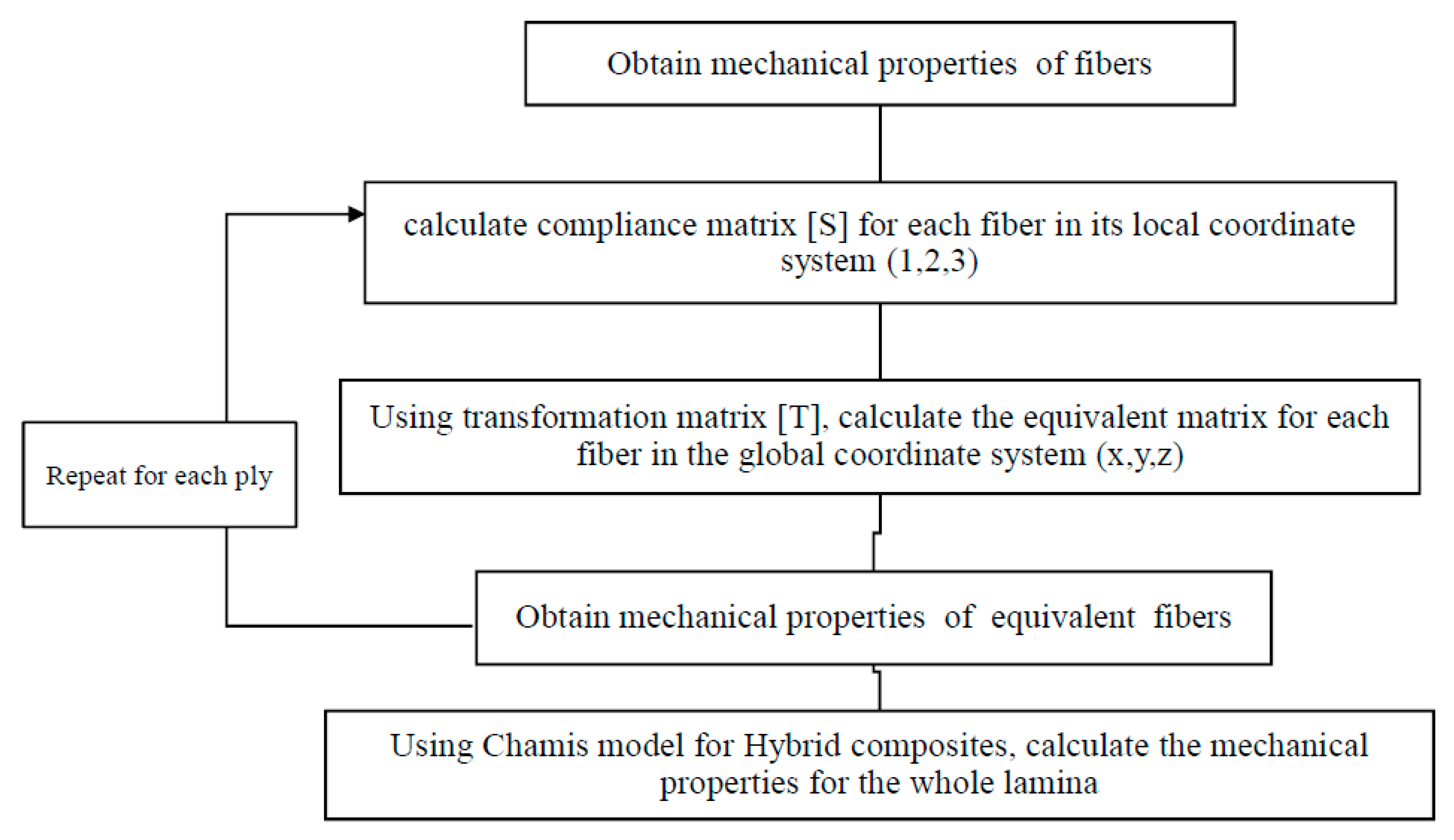
The compliance matrix [S] for each fiber in its local coordinate system (1,2,3) was calculated. Using transformation matrix [T], the equivalent matrix for each fiber in the global coordinate system (x,y,z) was calculated [27]. The mechanical properties of equivalent fibers were obtained. Using Chamis model for hybrid composites, the mechanical properties of the whole lamina were calculated.

$$E_1={\sum }_{i=1}^n{E^{\mathrm{fi}}}_{\mathrm{i}}{V}^{\mathrm{fi}}+E^{\mathrm{m}}{\mathrm{V}}^{\mathrm{m}},E_2=E_3=E^{\mathrm{m}}\left[\frac{1+1.165·{\sum }_{i=1}^n {\eta }^{\mathrm{fi}}{V}^{\mathrm{fi}}}{1-{\sum }_{i=1}^n {\eta }^{\mathrm{fi}}{V}^{\mathrm{fi}}}\right]$$

(28)

$${\eta }^{\mathrm{fi}}=\frac{\frac{E^{\mathrm{fi}}}{E^{\mathrm{m}}}-1}{\frac{{E^{\mathrm{fi}}}_{\mathrm{i}}}{E^{\mathrm{m}}}+1.165}$$

(29)

$$G_{23}=G^{\mathrm{m}}\left[\frac{1+0.9·{\sum }_{i=1}^n {\eta }^{\mathrm{fi}}{V}^{\mathrm{fi}}}{1-{\sum }_{i=1}^n {\eta }^{\mathrm{fi}}{V}^{\mathrm{fi}}}\right], G_{13}=G_{12}=G^{\mathrm{m}}\left[\frac{1+1.01·{\sum }_{i=1}^n {\eta }^{\mathrm{fi}}{V}^{\mathrm{fi}}}{1-{\sum }_{i=1}^n {\eta }^{\mathrm{fi}}{V}^{\mathrm{fi}}}\right]$$

(30)

$${\zeta }^{\mathrm{fi}}=\frac{\frac{{G^{\mathrm{fi}}}_{\mathrm{i}}}{G^{\mathrm{m}}}-1}{\frac{{G^{\mathrm{fi}}}_{\mathrm{i}}}{G^{\mathrm{m}}}+1.01}$$

(31)

where subscripts m and fi designate the matrix and the fibers, respectively; E₂ is the transverse Young’s modulus, G₁₂ is the in-plane shear modulus, V is the volume fraction, and ξ is a parameter associated with the fiber geometry (for circular fibers, it is 1.165 and 1.01).

It is noted that the fiber volume fraction should be divided into a number of plies so that their sum should be equal with the matrix volume fraction (the percentage of fiber volume in the entire volume of a fiber-reinforced composite material) up to 100%.

2.2. Principal Globalization

Generally, a laminate does not consist only of unidirectional laminae because of their low stiffness and strength properties in the transverse direction. Therefore, in most laminates, some laminae are placed at an angle (Figure 4) It is thus necessary to develop the stress–strain relationship for an angle lamina. The coordinate system is used for showing an angle lamina. The axes in the 1–2 coordinate system are called the local axes or the material axes. The direction 1 is parallel to the fibers, and the direction 2 is perpendicular to the fibers. In some references, direction 1 is also called the longitudinal direction L, and the direction 2 is called the transverse direction T. The axes in the x–y coordinate system are called the global axes or the off-axes. The angle between the two axes is denoted by angle θ.

The global and local stresses in an angle lamina are related to each other through the angle of the lamina θ:

$$\left[\begin{array}{c}\sigma x\\ \sigma y\\ \tau xy\end{array}\right]=\left[T\right]·\left[\begin{array}{c}{\sigma }_1\\ {\sigma }_2\\ {\tau }_{12}\end{array}\right],$$

(32)

where [T] is called the transformation matrix.

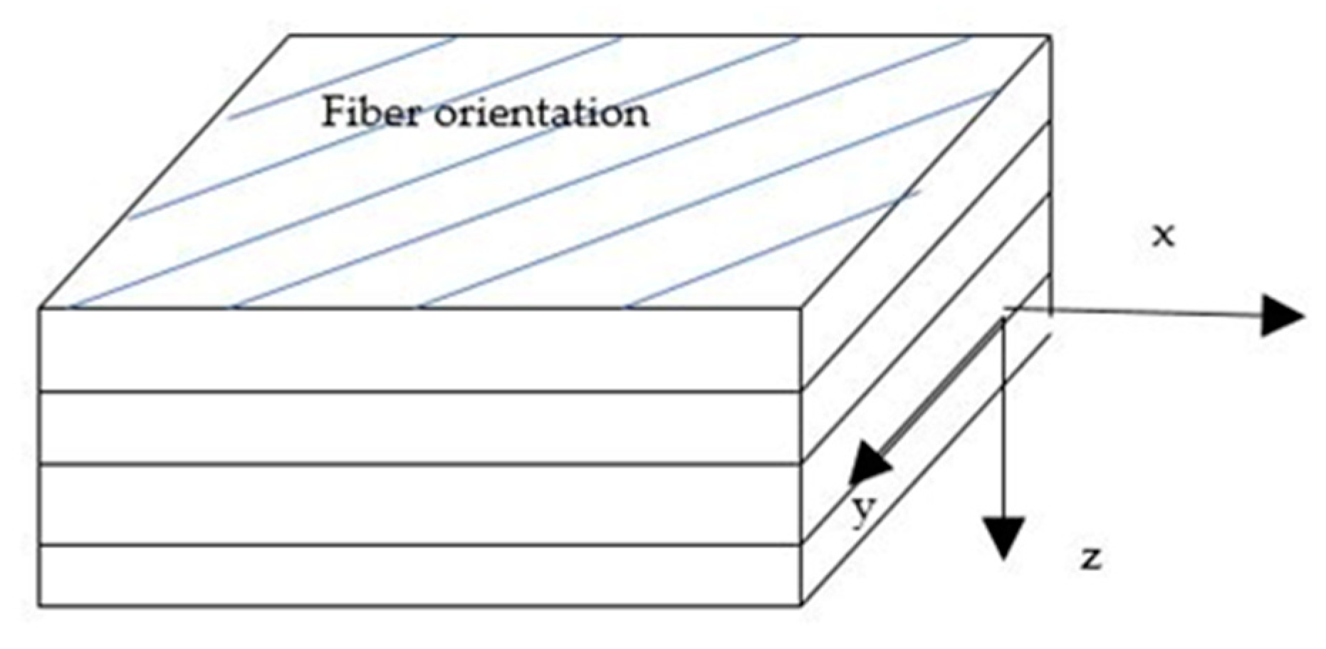
The mechanical properties of a typical unidirectional lamina are severely limited in the transverse direction. If one stacks several unidirectional layers (Figure 5) this may be an optimum laminate for unidirectional loads. However, for complex loading and stiffness requirements, this would not be desirable. This problem can be overcome by making a laminate with layers stacked at different angles for given loading and stiffness requirements. This approach increases the cost and weight of the laminate, and thus, it is necessary to optimize the ply angles. Moreover, layers of different composite material systems may be used to develop a more optimum laminate.

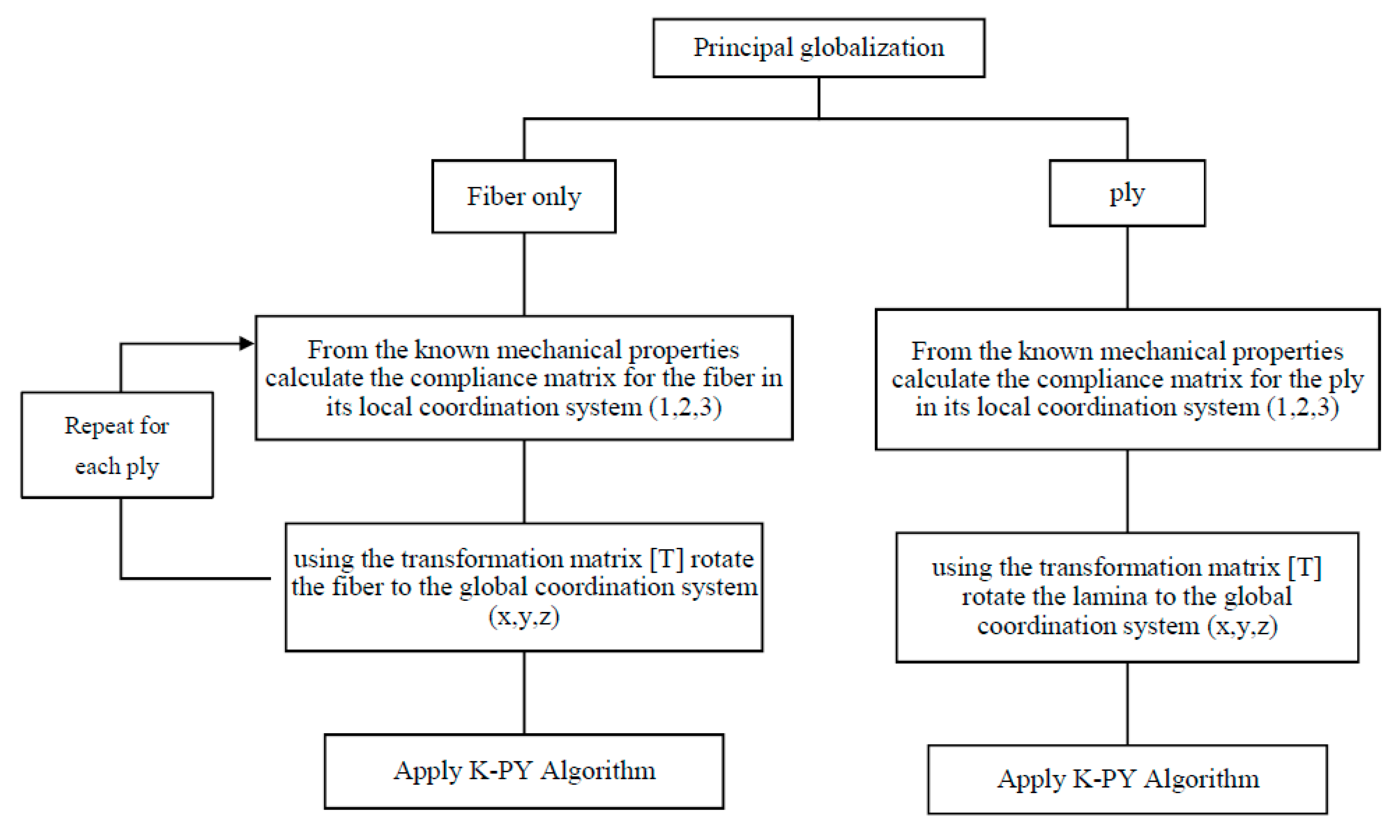
The idea is simply to find the equivalent lamina (or fiber) in order to be able to have a stack of laminae in the same direction. This equivalent can be found in two different ways (Figure 6).

Algorithm:

Figure 6. Algorithm Principal Globalization.

Figure 6. Algorithm Principal Globalization.

2.3. Thickness

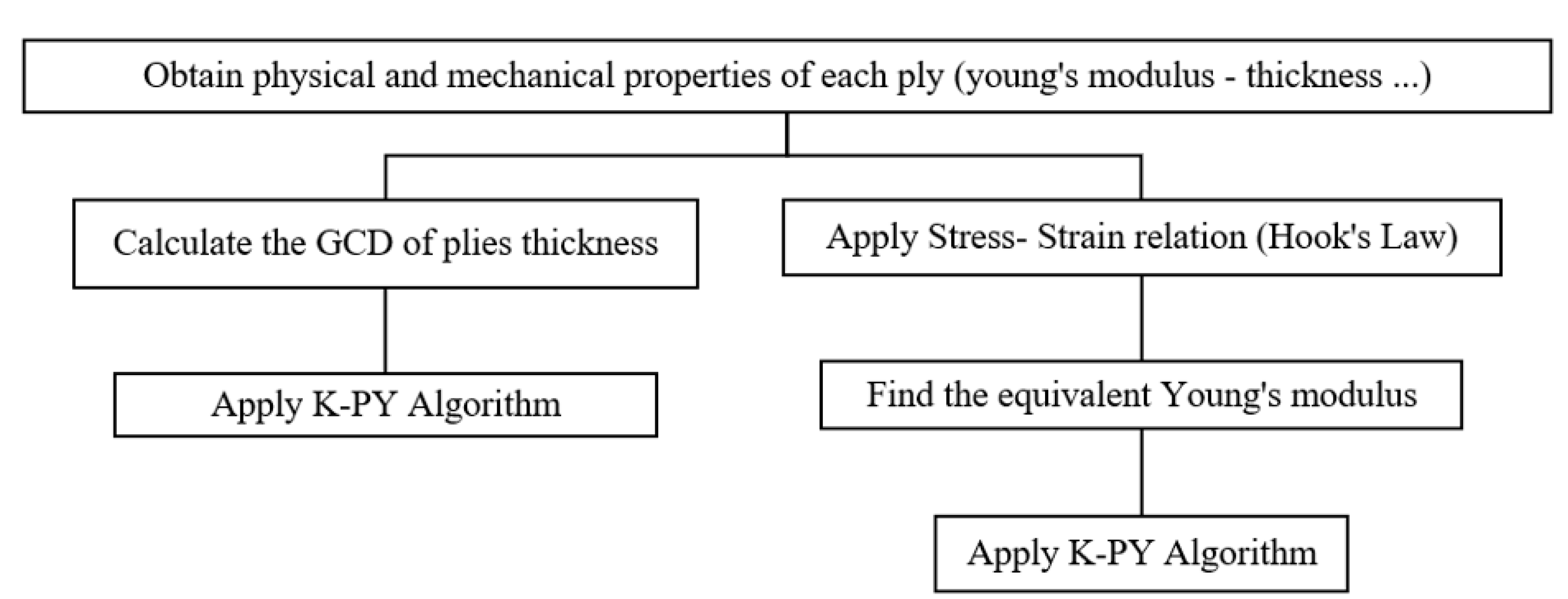
Size effects influence not only the strength of individual fibers, but also the longitudinal tensile strength and failure process of composite specimens and structures [28,29]. Most authors agree that the statistics of fiber strength are essential for establishing the relationship between the composite longitudinal tensile strength and size; in addition, other sources of size effects [30,31,32,33,34,35] are often considered as well. Size effects pose a challenge for the design of large composite structures based on experimental data measured in small coupons, and predictive models are therefore of utmost importance. This section suggests a generalized method for equivalence in thickness of laminate composites (Figure 7).

Algorithm:

Figure 7. Algorithm Thickness Method.

Figure 7. Algorithm Thickness Method.

2.3.1. GCD of Plies

This idea is simply based on finding the GCD for the thicknesses in composite materials in order to unify the thicknesses provided. The GCD with two or more integers, which are not all zero, is the largest positive integer that divides each of the integers. By calculating the GCD, the number of plies is equal to the initial thickness, and thus, we replaced the initial thickness with a number of plies with a uniform thickness, even if the composite materials have different types of fibers or matrices.

2.3.2. Stress–Strain Relation (Hook’s Law Method)

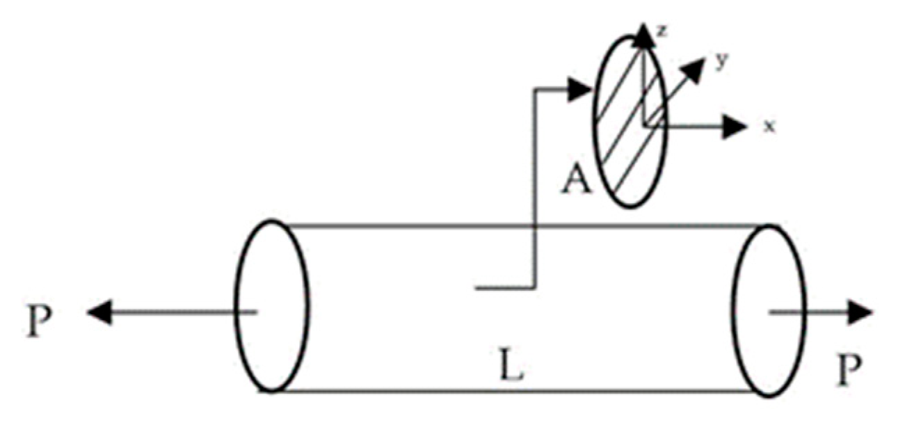
A mechanical structure takes external forces, which act upon a body as surface forces (for example, bending a stick) and body forces (for example, the weight of a standing vertical telephone pole on itself). These forces result in internal forces inside the body. Knowledge of the internal forces at all points in the body is essential because these forces need to be less than the strength of the material used in the structure. Stress, which is defined as the intensity of the load per unit area, determines this knowledge because the strengths of a material are intrinsically known in terms of stress. The determination of stress distributions of beams in necessary for determining the level of performance for the component. In particular, stress-based failure theories require determination of the maximum combined stresses in which the complete stress state must be either measured or calculated. Consider a bar of cross-section A and length L (Figure 8). A uniform tensile load P is applied to the two ends of the rod; by finding the state of stress, and strain energy per unit volume of the body. Assume that the rod is made of a homogeneous isotropic material of Young’s modulus, E. Normal Stress: Having derived the proportionality relation for strain, ε_x, in the x-direction, the variation of stress, σ_x

Using generalized Hook’s law:

$$\left[\begin{array}{c}{\epsilon }_{11}\\ {\epsilon }_{22}\\ {{\rm Y}}_{12}\end{array}\right]=\left[\begin{array}{ccc}\frac{1}{E_1}& \frac{-v_{12}}{E_2}& 0\\ \frac{-v_{12}}{E_1}& \frac{1}{E_2}& 0\\ 0& 0& \frac{1}{G_{12}}\end{array}\right]·\left[\begin{array}{c}{\sigma }_{11}\\ {\sigma }_{22}\\ {\tau }_{12}\end{array}\right]$$

(33)

$${\epsilon }_{11}=\frac{{\sigma }_{11}}{E_1}-\frac{v_{12}·{\sigma }_{22}}{E_2}$$

(34)

$${\epsilon }_{22}=-\frac{v_{12}·{\sigma }_{11}}{E_1}+\frac{{\sigma }_{22}}{E_2}$$

(35)

$${{\rm Y}}_{12}=\frac{{\tau }_{12}}{G_{12}}$$

(36)

Since the whole idea is to find equivalent

$${\epsilon }_{11}\left(\mathrm{eq}\right)=\frac{{\sigma }_{11}\left(\mathrm{eq}\right)}{E_1\left(\mathrm{eq}\right)}-\frac{{\nu }_{12}·{\sigma }_{22}\left(\mathrm{eq}\right)}{E_2\left(\mathrm{eq}\right)}$$

(37)

$${\epsilon }_{22}\left(\mathrm{eq}\right)=-\frac{{\nu }_{12}·{\sigma }_{11}\left(\mathrm{eq}\right)}{E_1\left(\mathrm{eq}\right)}+\frac{{\sigma }_{22}\left(\mathrm{eq}\right)}{E_2\left(\mathrm{eq}\right)}$$

(38)

$${{\rm Y}}_{12}\left(\mathrm{eq}\right)=\frac{{\tau }_{12}\left(\mathrm{eq}\right)}{G_{12}\left(\mathrm{eq}\right)}$$

(39)

where:

$${\sigma }_{11}=\frac{6FL}{bh2}$$

(40)

$${\sigma }_{22}=\frac{6Fb}{Lh2}$$

(41)

$${\tau }_{12}=\frac{F}{bh}$$

(42)

Since

$${\epsilon }_{11}={\epsilon }_{11}\left(\mathrm{eq}\right),{\epsilon }_{22}={\epsilon }_{22}\left(\mathrm{eq}\right),{{\rm Y}}_{12}={{\rm Y}}_{12}\left(\mathrm{eq}\right)$$

(43)

$$\frac{{\sigma }_{11}}{E_1}-\frac{v_{12}·{\sigma }_{22}}{E2}=\frac{{\sigma }_{11}\left(\mathrm{eq}\right)}{E_1\left(\mathrm{eq}\right)}-\frac{v_{12}·{\sigma }_{22}\left(\mathrm{eq}\right)}{E_2\left(\mathrm{eq}\right)}$$

(44)

$$-\frac{v_{12}·{\sigma }_{11}}{E_1}+\frac{{\sigma }_{22}}{E_2}=-\frac{v_{12}·{\sigma }_{11}\left(\mathrm{eq}\right)}{E_1\left(\mathrm{eq}\right)}+\frac{{\sigma }_{22}\left(\mathrm{eq}\right)}{E_2\left(\mathrm{eq}\right)}$$

(45)

$$\frac{{\tau }_{12}}{G_{12}}=\frac{{\tau }_{12}\left(\mathrm{eq}\right)}{G_{12}\left(\mathrm{eq}\right)}$$

(46)

And From Equations (38)–(43), we have:

$$\frac{L}{b}\times \frac{1}{h^2\left(eq\right)·E_{11}\left(eq\right)}-\frac{v_{21}·b}{L}\times \frac{1}{h^2\left(eq\right)·E_{22}\left(eq\right)}=\frac{L}{b}\times \frac{1}{h^2·E_{11}}-\frac{v_{21}·b}{L}\times \frac{1}{h^2·E_{22}}$$

(47)

$$-\frac{{\mathit{v}}_{21}·\mathit{L}}{\mathit{b}}\times \frac{\mathbf{1}}{{\mathit{h}}^{\mathbf{2}}\left(\mathit{e}\mathit{q}\right)·{\mathit{E}}_{11}\left(\mathit{e}\mathit{q}\right)}+\frac{\mathit{b}}{\mathit{L}}\times \frac{\mathbf{1}}{{\mathit{h}}^2\left(\mathit{e}\mathit{q}\right)·{\mathit{E}}_{22}\left(\mathit{e}\mathit{q}\right)}=-\frac{{\mathit{v}}_{21}·\mathit{L}}{\mathit{b}}\times \frac{1}{h^2·E_{11}}+\frac{b}{L}\times \frac{\mathbf{1}}{{\mathit{h}}^2·{\mathit{E}}_{22}}$$

(48)

Assuming that:

$$\mathsf{\alpha }=\frac{\mathit{L}}{\mathit{b}}\times \frac{\mathbf{1}}{{\mathit{h}}^2·{\mathit{E}}_{11}}-\frac{{\mathit{\nu }}_{21}·\mathit{b}}{\mathit{L}}\times \frac{\mathbf{1}}{{\mathit{h}}^2·{\mathit{E}}_{22}}$$

(49)

$$\mathsf{\beta }=-\frac{{\mathit{v}}_{21}·\mathit{L}}{\mathit{b}}\times \frac{1}{h^2·E_{11}}+\frac{b}{L}\times \frac{1}{h^2·E_{22}}$$

(50)

Therefore, the solution of Equations (44)–(46) is:

$$\frac{1}{E_{11}\left(eq\right)}=h^2\left(eq\right)·(\frac{ \alpha b\left(b-v{2}_{21}\left(L-b\right)\right)+v_{21}\beta b2}{bL-v{2}_{21}L2})$$

(51)

$$\frac{1}{E_{22}\left(eq\right)}=h^2\left(eq\right)·\left(\frac{v_{21}·\alpha +\beta }{\frac{b}{L}-v{2}_{21}}\right)$$

(52)

$$G_{12}\left(\mathrm{eq}\right)=\frac{h·G_{12}}{h\left(eq\right)}$$

(53)

3. Materials

In order to verify the applicability of this analytical model based on the equivalence in thickness, a model with two different ply is used in this work. A comparison between the results of present modeling, experimental data and previously developed multi-scale modeling. Four different examples are generated. As case studies, different mechanical properties are considered and the results are extracted.

3.1. UD—Homogenization

In order to verify the applicability of the analytical models, three types of examples were chosen from the specimens studied by Toledo and Menezes and their co-workers [32] to calculate the engineering elastic constants of laminate composites.

The laminates studied in this section are the following:

• Glass/epoxy [0/0] laminate;
• Silenka E-Glass 1200 tex MY750/HY917/DY063 epoxy [0/90]s laminate;
• Silenka E-Glass 1200 tex/MY750/HY917/DY063 epoxy [+45/−45]s laminate;
• E-Glass 21xK43 Gevetex/LY556/HT907/DY063 [+90/+30/−30]s laminate.

Elastic properties of fibers and matrices are shown in [32,33].

3.2. Principal Globalization

A three-ply [0/90]s graphite/epoxy laminate with elastic properties as shown in

Table 1. Elastic properties of fibers.

Fibers (GPa)
E-Glass Ef11 = Ef22 = 72.4; Gf12 = 30.2; νf23 = 0.2
Silenka E-Glass 1200 tex Ef11 = Ef22 = 74; Gf12 = 30.2; νf23 = 0.2
E-Glass 21xK43 Gevetex Ef11 = Ef22 = 80; Gf12 = 30.2; νf23 = 0.2

and

Table 2. Elastic properties of matrices.

Matrices
Epoxy Em = 2.76; Gm = 1.567; νm = 0.35
MY750/HY917/DY063 epoxy Em = 3.35; Gm = 1.24; νm = 0.35
LY556/HT907/DY063 Em = 3.35; Gm = 1.24; νm = 0.35

:

3.3. Equivalence in Thickness

The elastic properties of the materials are derived from

Table 3. Elastic properties of fibers and matrices.

Graphite/Epoxy Laminate Properties
Vf = 0.7
E1 = 181
E2 = E3 = 10.3
G12 = G13 = 7.17
G23 = 5.79
ν12 = ν13 = 0.28

and

Table 4. Elastic properties of fibers and matrices.

Property	E-Glass/Epoxy Laminate	Carbon Fiber/Epoxy Laminate
Vf	0.6	0.6
E1	45.6	126
E2 = E3	16.2	11
G12 = G13	5.83	6.6
G23	5.79	3.93
ν12 = ν13	0.278	0.28
ν23	0.4	0.4

[36].

4. Results and Discussion

With the purpose of validating the developed modeling technique, the results were compared with experimental data published in open literature. A comparison between the results of present modeling, experimental data, and previously developed multi-scale modeling was conducted. As case studies, different mechanical properties were considered, and the results are shown in

Table 5. Ex Young’s modulus comparison.

Type of Composite	Orientation	Experimental	Norm 0	Norm ∞	Norm Cart.	Norm 3	Norm 4	Hybrid Method
Glass/epoxy	[0/0]	56	55.14	55.14	55.14	55.14	32.39	50
E-Glass 1200 tex MY750/HY917/DY063 epoxy	[0/90]s	29.2	12.564	45.74	29.152	29.152 ± 16.58i	24.14	31.19
E-Glass 1200 tex MY750/HY917/DY063 epoxy	[+45/−45]s	14.4	12.72	12.72	12.72	12.72	7.471	16.511
E-Glass/LY556/HT907/DY063	[+90/+30/−30]s	27.4	12.52	29.12	28.8766	28.8766 ± 13.085i	21.71	30.633

,

Table 6. Ey Young’s modulus comparison.

Type of Composite	Orientation	Experimental	Norm 0	Norm ∞	Norm Cart.	Norm 3	Norm 4	Hybrid Method
Glass/epoxy	[0/0]	15	18.18	18.18	18.18	18.18	10.679	13
E-Glass 1200 tex MY750/HY917/DY063 epoxy	[0/90]s	17.2	12.86	21.673	17.2665	17.2 ± 4.4064i	11.155	21.476
E-Glass 1200 tex MY750/HY917/DY063 epoxy	[+45/−45]s	17.1	18.67	18.67	18.67	18.67	10.966	21.281
E-Glass/LY556/HT907/DY063	[+90/+30/−30]s	22.3	12.55	39.154	24.401	24.401 ± 11.05i	18.623	27.374

,

Table 7. Gxy Shear modulus comparison.

Type of Composite	Orientation	Experimental	Norm 0	Norm ∞	Norm Cart.	Norm 3	Norm 4	Hybrid Method
Glass/epoxy	[0/0]	3	2.57	2.57	2.57	2.57	1.5	5.5
E-Glass 1200 tex MY750/HY917/DY063 epoxy	[0/90]s	5.83	4.832	6.464	5.648	5.648 ± 0.816i	3.428	3.7876
E-Glass 1200 tex MY750/HY917/DY063 epoxy	[+45/−45]s	10.6	7.047	7.047	7.047	7.047	4.14	5.6186
E-Glass/LY556/HT907/DY063	[+90/+30/−30]s	5.79	5	6.43	5.66	5.66 ± 0.588i	3.383	3.924

,

Table 8. Engineering constants comparison.

Engineering Constants (GPa)	Kaw	Fiber Method	PLY Method
Ex	124.5	124.728	126.828
Ey	67.43	68.27	69.25
Gxy	7.17	7.55	7.64

,

Table 9. Ex Young’s modulus comparison.

Type of Composite	Thickness (mm)	CLT Experimental	GCD Method	Hook’s Law Method
G–G–G–G–G–G	0.05–0.03	46.875	46.54	44.1
C–C–C–C–C–C	0.05–0.03	126.857	127.104	122.458
G–G–C–C–G–G	0.05–0.03	65.346	73.39	61.56
C–C–G–G–C–C	0.05–0.03	108.42	100.25	101.75

,

Table 10. Ey Young’s modulus comparison.

Type of Composite	Thickness (mm)	CLT Experimental	GCD Method	Hook’s Law Method
G–G–G–G–G–G	0.05–0.03	16.658	18.2	17.674
C–C–C–C–C–C	0.05–0.03	11.07	10.29	11.358
G–G–C–C–G–G	0.05–0.03	15.369	15.563	15.90
C–C–G–G–C–C	0.05–0.03	12.365	12.92	12.983

and

Table 11. Gxy Shear modulus comparison.

Type of Composite	Thickness (mm)	CLT Experimental	GCD Method	Hook’s Law Method
G–G–G–G–G–G	0.05–0.03	5.83	5.89	6.72
C–C–C–C–C–C	0.05–0.03	6.6	6.81	7.61
G–G–C–C–G–G	0.05–0.03	6	6.19	7.55
C–C–G–G–C–C	0.05–0.03	6.423	6.5	7.63

, each of which shows a clear comparison between the experimental results and the presented algorithm.

For example, Table 5, Table 6, Table 7, Table 8, Table 9, Table 10 and Table 11 show the comparison of longitudinal and transversal Young’s moduli and shear modulus between four different materials and fibers with different orientations and the two methods suggested in the UD-homogenization section of the K-PY algorithm, as well as a comparison implied between the two suggested methods, which are the 5 norms and the hybrid method.

On the other hand, Table 8 shows a clear comparison for the section of principal globalization and compares the results not only with experimental results with the literature but also those between the two suggested algorithms, i.e., the fiber method and the PLY method.

Finally, Table 9, Table 10 and Table 11 show comparisons related to the thicknesses study methods with the classical laminate theory and the two suggested methods by the author, i.e., the GCD and the hook’s law method.

4.1. UD—Homogenization

For all case studies, the fiber volume fraction was considered constant in all layers. The obtained results are presented in Table 5, Table 6 and Table 7.

As it was predicted, norm 0 shows lower results among the five presented models, while norm ∞ was the highest. The Cartesian norm was the most accurate between all presented methods due to its direct relation to Chamis model, as discussed earlier. Norm 3 is not dependable, since its solution is always imaginary at ply number that exceeds two due to the Cauchy-Schwarz inequality [19], but it is notable that the real part is similar to the Cartesian norm because it is a second-order equation. Norm 4 and the hybrid method were not as efficient as the Cartesian norm.

It was observed that the Young’s modulus in direction 1 is the most accurate parameter up to 0.1% (in comparison with that in the second experiment) for the longitudinal Young’s modulus Ex, and that the maximum average error is shown for the Cartesian Norm model with 4.55%. For the transverse Young’s modulus the percentage of error is much higher than for the longitudinal Young’s modulus, with an average of 10.2% (the minimum percentage of error was for the second experiment with 0.38%). In addition, the average percentage of error for shear modulus in the Cartesian norm was 13.2% (with 2.24% as the lowest value from experiment 4).

Moreover, the percentage of errors with the hybrid method was higher, so their results are shown and not dependent on the ultimate path of the K-PY algorithm.

In addition to the high accuracy level of the current modeling technique, the very short runtime required of the modeling renders the developed multi-scale modeling as a cost-effective computational tool for estimating the Young’s moduli of laminate composites.

4.2. Principal Globalization

Since the Cartesian norm was the most accurate among all presented methods, a clear comparison between the experimental values presented by Kaw [26] and the predicted results from the K-PY Equivalence model was implemented.

As shown in Table 8, the comparison was focused on Young’s modulus Ex, Ey and Shear modulus Gxy. The fiber method present more accurate and precise values with the percentages of error varied from 0.128% for longitudinal Young’s modulus Ex, 1.23% for transversal Young’s modulus Ey, and 5% for Shear modulus Gxy, while the PLY method shows higher percentages of errors, such as 2.6% for Ex, 2.62% for Ey, and 6.15% for Gxy.

4.3. Equivalence in Thickness

The obtained results are presented in Table 9, Table 10 and Table 11.

Table 9, Table 10 and Table 11 give a clear comparison between the experimental values and the predicted results from the present K-PY Equivalence in thickness model in both GCD and Hook’s law methods. The comparison was focused on Young’s moduli Ex, Ey, and shear modulus Gxy. From Table 9 and Table 10, good agreement was obtained between the predicted results and the available experimental values of the GCD method. The relative errors for the Young’s moduli were 5.18% and 6.02%, respectively, while for Hook’s law method they were around 5.52% and 4.03%, respectively. Moreover, the relative error for shear modulus Gxy was 2.1% for the GCD method, while for Hook’s law method it was around 18.7%. As illustrated in Table 9, Table 10 and Table 11, as for the comparison of Young’s modulus, it can be seen that the result were greater than the experimental values by about 5–6% for the GCD method while for Hook’s law method it was greater than 4–5%. Similarly, the result for shear modulus Gxy was 2.1% for the GCD method while for Hook’s law method it was greater than18%. From the aforementioned analysis, the contribution of K-PY Equivalence in thickness model in the GCD method can be taken into account for precisely predicting the elastic properties. The results showed that the present analytical model based on finding equivalent and with the application of thickness uniformity can be used to effectively evaluate the elastic properties for laminate composites.

5. Conclusions

The constitutive models presented in this paper are able to reproduce the behavior of laminated composites formed by fiber-reinforced laminae with different orientations or different types of fibers. The suggested hypotheses are the simplest that can be applied to isotropic fibers. As it was shown in the methodology section, applying the algorithm is easy and simple. Other models were also presented to discuss the equivalence of fibers or ply from the perspective of angle or thickness.

Good agreement was observed among numerical results, with smaller differences in the transversal strains, as shown in the results section that the Young’s modulus in direction 1 was the most accurate parameter up to 0.1% (in comparison with that from the second experiment) for the longitudinal Young’s modulus Ex and that the maximum average error is shown for the Cartesian norm model with 4.55% but with an average percentage of error of transversal strains of 10.2% (the minimum percentage of error was 0.38% for the second experiment); this can be due basically to the lack of precision in the mechanical properties of the components, fundamentally of the fibers, used as input data.

In general, application examples and comparisons with experimental results showed that the models are able to properly reproduce the mechanical behaviors of laminae and composite laminates. The models also describe the failure of the composite, taking into account what happens in each component. It also allows identifying the failure mode of the composite, produced by the failure of one or more of its components. It is able to reproduce complex failure modes that change from the matrix to the fibers as shown for equivalence in thicknesses and orientation where the percentages of errors were only up to 2% and less from results section in all predicted Young’s and shear moduli, since only in equivalence in thicknesses the highest value of error was 5% for Gxy, depending on the type of stress state. The model works better for some types of laminates, and further analysis and model calibration are needed.

The models were covered in the paper, based directly on Chamis model with an objective function for optimization and hybrid-based model that discuss the equivalence of fiber in angle. The equivalence in orientation and in thickness was also discussed in this paper, and a new Generalization model was presented. The framework presented is potentially valid for other fiber conditions such as fiber volume fraction, but these cases would require further development.

Ultimately, it is concluded that the most accurate path to predict and reproduce the behavior of laminated composites in the orientation case is to apply the rotation/equivalence on fiber and then to apply K-PY model using the Objectif function with the Cartesian norm. While for equivalence in thickness, it was concluded that the GCD method is the most accurate method to use. As shown in the results, all values from Table 5, Table 6, Table 7, Table 8, Table 9, Table 10 and Table 11 had relatively low percentages of error, differing from 0.128% as shown in Table 8. The percentage is related to the lack of the exact and precise database structure of the used material, but it does show a great capability to use the algorithm to find the ultimate and optimal solution. This algorithm (Figure 9) is easily adaptable to laminates with periodicity, such as multi-angle lay-up composites. This algorithm allows researchers and end users to calculate the stiffness and compliance matrix of any composite material, with any form, orientation, or thickness, saving so much time and cost while finding the optimal solution.

Optimal Path Algorithm:

Figure 9. Optimal Path Algorithm.

Figure 9. Optimal Path Algorithm.

References

1. Daniel, G.; Suong, V.H.; Tsai, W.S. Composite Materials: Design and Applications; CRC Press: Boca Raton, FL, USA, 2003. [Google Scholar]
2. Chamis, C.C. Mechanics of composite materials: Past, present, and future. J. Compos. Technol. Res. 1989, 11, 3–14. [Google Scholar]
3. Sanjay, K.M. Composites Manufacturing: Materials, Product and Engineering; CRC Press: Boca Raton, FL, USA, 2002. [Google Scholar]
4. Ogin, S.L.; Brøndsted, P.; Zangenberg, J. Composite Materials: Constituents, Architecture, and Generic Damage Modeling Damage, Fatigue and Failure of Composite Materials; Woodhead Publishing: Sawston, UK, 2016; pp. 3–23. [Google Scholar]
5. Richardson, D. The Fundamental Principles of Composite Material Stiffness Predictions; University of the West England: Bristol, UK, 2011. [Google Scholar]
6. Lydzba, D. Effective Properties of Composites, Introduction to Micromechanics; Wroclaw University of Technology: Wrocław, Poland, 2011. [Google Scholar]
7. Chan, W.S. Equivalent thermal expansion coefficients of lumped layer in laminated composites. Compos. Sci. Technol. 2006, 66, 2402–2408. [Google Scholar] [CrossRef]
8. Kumar, G.; Shapiro, V. Efficient 3D analysis of laminate structures using ABD-equivalentmaterial models. Finite Elem. Anal. Des. 2015, 106, 41–55. [Google Scholar] [CrossRef] [Green Version]
9. Yin, H.; Zhao, Y. Introduction to the Micromechanics of Composite Materials, 1st ed.; CRC Press: Boca Raton, FL, USA, 2016. [Google Scholar]
10. Dixit, A.; Mali, H.S.; Misra, R.K. Unit cell model of woven fabric textile composite for multiscale analysis. Procedia Eng. 2013, 68, 352–358. [Google Scholar] [CrossRef] [Green Version]
11. Kuksenko, D.; Böhm, H.J.; Drach, B. Effect of micromechanical parameters of composites with wavy fibers on their effective response under large deformations. Adv. Eng. Softw. 2018, 121, 206–222. [Google Scholar] [CrossRef]
12. Nazarenko, L.; Stolarski, H.; Altenbach, H. Thermo-elastic properties of random composites with unidirectional anisotropic short-fibers and interphases. Eur. J. Mech. A Solids 2018, 70, 249–266. [Google Scholar] [CrossRef]
13. Banerjee, S.; Sankar, B.V. Mechanical properties of hybrid composites using finite element method based micromechanics. Compos. Part B Eng. 2014, 58, 318–327. [Google Scholar] [CrossRef]
14. Chamis, C.C.; Sinclair, J.H. Mechanics of intraply hybrid composites—Properties, analysis, and design. Polym. Compos. 1980, 1, 7–13. [Google Scholar] [CrossRef]
15. Chou, T.-W. Microstructural Design of Fiber Composites; Cambridge University Press: Cambridge, UK, 1992. [Google Scholar]
16. Halpin, J.C.; Kardos, J.L. The Halpin-Tsai equations: A review. Polym. Eng. Sci. 1976, 16, 344–352. [Google Scholar]
17. Swolfs, Y.; Gorbatikh, L.; Verpoest, I. Fibre hybridisation in polymer composites: A review. Compos. Part A Appl. Sci. Manuf. 2014, 67, 181–200. [Google Scholar] [CrossRef]
18. Henry, J.; Pimenta, S. Modelling hybrid effects on the stiffness of aligned discontinuous composites with hybrid fibre-types. Compos. Sci. Technol. 2017, 152, 275–289. [Google Scholar] [CrossRef]
19. Minculete, N.; Moradi, H.R. Some Improvements of the Cauchy-Schwarz Inequality Using the Tapia Semi-Inner-Product. Mathematics 2020, 8, 2112. [Google Scholar] [CrossRef]
20. Escalante-Solís, M.A.; Valadez-González, A.; Herrera-Franco, P.J. A note on the effect of the fiber curvature on the micromechanical behavior of natural fiber reinforced thermoplastic composites. Express Polym. Lett. 2015, 9, 1119–1132. [Google Scholar] [CrossRef]
21. Hassanzadeh-Aghdam, M.K.; Ansari, R.; Mahmoodi, M.J. Micromechanical estimation of biaxial thermomechanical responses of hybrid fiber-reinforced metal matrix nanocomposites containing carbon nanotubes. Mech. Mater. 2018, 119, 1–15. [Google Scholar] [CrossRef]
22. Wisnom, M.R.; Khan, B.; Hallett, S.R. Size effects in unnotched tensile strength of unidirectional and quasi-isotropic carbon/epoxy composites. Compos. Struct. 2008, 84, 21–28. [Google Scholar] [CrossRef]
23. Anto, A.D.; Mia, S.; Hasib, M.A. The influence of number and orientation of ply on tensile properties of hybrid composites. J. Phys. Mater. 2019, 2, 025002. [Google Scholar] [CrossRef]
24. Dobah, Y.; Ghazzawi, Y.; Bourchak, M. Mechanical properties of hybrid carbon fibre reinforced polyethene and epoxy composites. ARPN J. Eng. Appl. Sci. 2015, 10, 7053–7057. [Google Scholar]
25. Parvanesh, V.; Shariati, M.; Nezakati, A. Statistical analysis of the parameters influencing the mechanical properties of layered MWCNTs/PVA nano composites. Int. J. Nano Dimens. 2015, 6, 509–516. [Google Scholar]
26. Kaw, A.K. Mechanics of Composite Materials, Mechanical and Aerospace Engineering Series; CRC Press: Boca Raton, FL, USA, 2005. [Google Scholar]
27. Bufler, H. Theory of elasticity of a multilayered medium. J. Elast. 1971, 1, 125–143. [Google Scholar] [CrossRef]
28. Rowe, R.K.; Booker, J.R. Finite layer analysis of nonhomogeneous soils. J. Eng. Mech. Div. 1982, 108, 115–132. [Google Scholar] [CrossRef]
29. Chatterjee, S.N.; Pindera, M.-J.; Pipes, R.B.; Dick, B. Composite Defect Significance; MSC TFR 1312/1108 (NADC Report No. 81034-60); Spring Hottse: Montgomery County, PA, USA, 1982; Available online: http://citeseerx.ist.psu.edu/viewdoc/download?doi=10.1.1.895.3671&rep=rep1&type=pdf (accessed on 1 September 2021).
30. Aboudi, J. Micromechanical analysis of thermo-inelastic multiphase short-fiber composites. Compos. Eng. 1995, 5, 839–850. [Google Scholar] [CrossRef] [Green Version]
31. Babu, P.E.J.; Savithri, S.; Pillai, U.T.S.; Pai, B.C. Micromechanical modeling of hybrid composites. Polymer 2005, 46, 7478–7484. [Google Scholar] [CrossRef]
32. Younes, R.; Hallal, A.; Fardoun, F.; Chehade, F.H. Comparative Review Study on Elastic Properties Modeling for Unidirectional Composite Materials. Compos. Prop. 2012, 17, 391–408. [Google Scholar]
33. Toledo, M.W.E.; Nallim, L.G.; Luccioni, B.M. A micro-macromechanical approach for composite laminates. Mech. Mater. 2008, 40, 885–906. [Google Scholar] [CrossRef]
34. de Menezes, E.A.W.; Eggers, F.; Marczak, R.J.; Iturrioz, I.; Amico, S.C. Hybrid composites: Experimental, numerical and analytical assessment aided by online software. Mech. Mater. 2020, 148, 103533. [Google Scholar] [CrossRef]
35. Soden, P.D.; Hinton, M.J.; Kaddour, A.S. Lamina properties, lay-up configurations and loading conditions for a range of fiber-reinforced composite laminates. Compos. Sci. Technol. 1998, 58, 1011–1022. [Google Scholar] [CrossRef]
36. Wisnom, M.R. Size effects in the testing of fibre-composite materials. Compos. Sci. Technol. 1999, 59, 1937–1957. [Google Scholar] [CrossRef]
Figure 1. All paths of K-PY algorithm.
Eng 02 00026 g001
Figure 2. Algorithm Objectif Function.
Eng 02 00026 g002
Figure 3. Algorithm Hybrid Method.
Eng 02 00026 g003
Figure 4. Local and global axes of an angle lamina.
Eng 02 00026 g004
Figure 5. Fibre orientation in a lamina.
Eng 02 00026 g005
Figure 8. Cross section of beam.
Eng 02 00026 g008