Accurate Empirical Calculation System for Predicting the Seepage Discharge and Free Surface Location of Earth Dam over Horizontal Impervious Foundation

Abstract

In the numerical analysis of the Laplace equation, which is the governing equation of the seepage phenomena of homogeneous, isotropic earth dams, it has been confirmed that numerical analysis with high accuracy is possible by using the interpolation finite difference method (IFDM). In a previous paper, based on this numerical analysis method, the equivalent Kozeny (KZ) flow method was proposed as a new empirical method to calculate the seepage discharges and free surface locations of earth dams. Although this method is generally a highly accurate method compared with the empirical method of A. Casagrande, owing to calculating the seepage problems within a few percentages of discharge relative errors, several additional studies are necessary. By integrating the finding of this study to the previous literature, an empirical seepage calculation system with high accuracy, the equivalent KZ flow method, is created. Owing to the finally proposed empirical method, called “interpolation-equivalent KZ flow method”, the discharge and free surface location can be predicted with high accuracy in a wide range.

1. Introduction

Conventionally, high-accuracy numerical analyses of seepage problems of earth dams have been implemented using the finite element method. Numerical analyses using the finite difference method (FDM) have been limited to cases where the calculation domains are comparatively simple. However, by applying the interpolation finite difference method (IFDM), two- and three-dimensional elliptic partial differential equations (PDEs) over complex domains with high speed and high accuracy can be freely solved [1,2,3] The IFDM is composed of two kinds of methods [3] (1) Algebraic Polynomial Interpolation Method (APIM), where finite difference schemes are formulated instantaneously over equally or unequally spaced grid points, and (2) Boundary Polynomial Interpolation Method (BPIM), where numerical calculations are executed only over equally spaced grid points, and the boundary interpolation is performed to match the boundary conditions. In the paper, the numerical calculations are executed by the IFDM-BPIM.

This method is adopted as a numerical analysis method for solving confined/unconfined seepage problems. In such problems, because of the adoption of IFDM-BPIM using the quadratic interpolation at the boundary, it has been shown that highly accurate numerical calculations are possible even in the FDM [4,5].

Empirical methods proposed in the first half of the previous century—(1) A. Casagrande method, (2) Schaffernak–Van Iterson method, and (3) L. Casagrande method—have been adopted in design standards [6,7] without sufficient verifications. Fukuchi (2018) [5] summarized the critique of these empirical methods as follows.

“Many researchers have pointed out various problems in A. Casagrande’s method, and some have proposed alternatives (Uginchus, 1960 [8]; Lo, 1971 [9]; Browzin, 1976 [10]). Several issues have since been raised. Shrivastava (2015) [11] suggested a modified equation for the phreatic line in an earthen dam, which is much more accurate than that given by A. Casagrande. Salmasi and Jafari (2016) [12] computed the locations of the free surface for 28 examples using the SEEP/W software (GEO-SLOPE 2009) [13] and found that, in most cases, the Schaffernak–Van Iterson method has more than 20% error and A. Casagrande’s method has more than 30% error. Using SEEP/W, Jamel (2016) [14] computed the discharges for 729 examples without a drain and found that A. Casagrande’s solution has more than 15% error.” Despite many criticisms of these empirical methods, attempts to construct a new empirical method have not yet been made.

The author has also confirmed that with these methods, even if the permissible error is set to 10%, sufficient calculation accuracy is not guaranteed. These empirical methods should be critically examined by comparing them with numerical calculation at its current state. In this study, an empirical estimation with a permissible error of a few percent is considered. With respect to discharge, it is defined that the absolute relative error of an empirical discharge ($q_e$) to the numerically calculated discharge ($q_n$) is within 3%; thereafter, the criterion is the numerically calculated discharge, specifically, $\left|q_e-q_n\right|/q_n\times 100\%\le 3\%$. With respect to the location of the free surface, the maximum calculation error usually occurs at the discharge point B and is evaluated by its vertical y-coordinate $yB$. The absolute relative error of an empirical discharge point $y{B}_e$ to the numerically calculated discharge point $y{B}_n$ is within 3%; thereafter, the criterion is the entrance face head H, specifically, $\left|y{B}_e-y{B}_n\right|/H\times 100\%\le 3\%$. The error-within-three-percent estimation means that both conditions are satisfied. In a previous paper [5], we mainly focused on the estimated discharge and discussed the calculation accuracy of the empirical method. In this study, the estimation accuracy, including the discharge point, is evaluated.

Even at this point in time, when the governing differential equations are instantaneously numerically analyzed, the author believes that highly accurate empirical methods are required to grasp the overall picture of seepage phenomena [5]. If conventional empirical methods have structural defects and a highly accurate prediction is impossible, then it is necessary to establish a better rule of thumb. From this viewpoint, an empirical method, the equivalent Kozeny (KZ) flow method, was proposed in the previous paper. The theory presented in this paper is inseparably associated with this concept.

In the following, Section 2 outlines the governing equation and its finite differential equation (FDE); regarding the detail numerical calculation method, refer to the previous two papers [4,5]. Section 3 shows the basic results of the equivalent KZ flow confirmed in the previous paper [8]. The empirical method of A. Casagrande was discussed in detail in the previous paper. Section 4 newly describes the numerical calculation results for (2) Schaffernak–Van Iterson method and (3) L. Casagrande method. Section 5 details the interpolation-equivalent KZ flow, which is the main subject of this paper. Section 6 summarizes the basic results of this paper and discusses the effectiveness of the proposed method. It is confirmed that the results of the proposed empirical methods agree with the numerical calculation results with high accuracy in almost all usual type isotropic homogeneous earth dams.

2. Governing Equation of Numerical Calculation

In our previous papers [4,5], numerical calculation methods based on the IFDM-BPIM were explained in detail. Here, the governing partial differential equation (PDE) and its FDE are verified. In the IFDM, the PDE for the potential calculation is the following parabolic PDE:

$$\frac{\partial h}{\partial t}=\frac{{\partial }^{2}h}{\partial x^2}+\frac{{\partial }^{2}h}{\partial y^2}\left(\equiv {\nabla }^{2}h\right)$$

(1)

where $h$ is the total head ($position head, y,+pressure head, p$) and $t$ denotes time; then, $\partial h/\partial t$ is the pseudo-acceleration term [5,15]. The $x$-direction is horizontal and the $y$-direction is vertical. Under a fixed boundary condition, as $t\to \infty$, $\partial h/\partial t\to 0,$ the equation reduces to the Laplace equation, ${\nabla }^{2}h=0$. The following expression describes the stream function, $s$:

$$\frac{\partial s}{\partial t}=\frac{{\partial }^{2}s}{\partial x^2}+\frac{{\partial }^{2}s}{\partial y^2}\left(\equiv {\nabla }^{2}s\right)$$

(2)

The numerical calculation methods for Equations (1) and (2) are the same; consider Equation (1). The Laplace equation, ${\nabla }^{2}h=0$, is usually calculated using the successive over relaxation (SOR) scheme. On the other hand, Equation (1) is usually solved by the forward time, centered space (FTCS) scheme. The FDE of the FTCS scheme is expressed as follows [4]:

$$h_{i,j}^{n+1}=h_{i,j}^n+{\phi }_{i,j}\Delta t\left[F_x^{″}\left(h_{i,j}^n\right)+F_y^{″}\left(h_{i,j}^n\right)\right], {\phi }_{i,j}\equiv {\left(l_{wi,j}\right)}^{p_w}$$

(3)

$$F_x^{″}\left(h_{i,j}^n\right)=\frac{h_{i-1,j}^n-2h_{i,j}^n+h_{i+1,j}^n}{{\left(\Delta x\right)}^2}$$

(3a)

$$F_y^{″}\left(h_{i,j}^n\right)=\frac{h_{i,j-1}^n-2h_{i,j}^n+h_{i,j+1}^n}{{\left(\Delta y\right)}^2}$$

(3b)

In the FTCS scheme, calculated variables are replaced simultaneously. However, if we are only interested in the convergence state, successive displacement of variables accelerates the convergence. This scheme is the time marching successive displacement (TMSD) scheme [2,4,15]. Changes from the former to the latter are carried out easily and instantaneously. Moreover, it has been confirmed that the TMSD scheme is exactly equivalent to the SOR scheme [16] limited as using the second-order centered space finite difference scheme [2,15]. In the paper, all calculations are carried out using the TMSD scheme.

In Equation (3), ${\phi }_{i,j}$ is the time-interval adjustment factor, and $l_{wi,j}$ is the wall-distance factor. In the definition of ${\phi }_{i,j}\equiv {\left(l_{wi,j}\right)}^{p_w}$ in Equation (3), $p_w=1$ is defined under the condition that the calculation element of concern is the near-wall element with $0<l_{wi,j}<1$, and the boundary condition is the Dirichlet condition. In all other cases, ${\phi }_{i,j}=1$ (namely, $p_w=0$) and Equation (3) reduce to the usual FDE [4]. The time interval is defined as follows:

$$\Delta t={\alpha }_b\Delta t_c, \Delta t_c\equiv \frac{1}{2}/\left[\frac{1}{{\left(\Delta x\right)}^2}+\frac{1}{{\left(\Delta y\right)}^2}\right],0<{\alpha }_b<{\alpha }_{b\max }$$

(4)

where ${\alpha }_b$ is the acceleration factor of the TMSD scheme, and ${\alpha }_{bmax}$ is the theoretical maximum acceleration factor. The stability condition $0<{\alpha }_b<{\alpha }_{bmax} \left(=2\right)$ ensures that the calculation has a convergent solution. It is advantageous to use the optimum acceleration factor, ${\alpha }_b={\alpha }_{bopt}$, to achieve the fastest convergence [2]. However, in this study, ${\alpha }_b= 1.80$ is adopted because this value guarantees stable convergence without exception.

3. Concept of Equivalent KZ Flow

In the previous paper [5], the concept of equivalent KZ flow was presented in detail. Because the theory employed in this study is intertwined with the concept, this section begins by confirming the basic contents presented in the previous paper. Kozeny (1931) [17] derived an analytical solution of the seepage phenomenon with a discharge angle $\mathsf{\alpha }=180$° (see Figure 1) by conformal mapping and showed that the free surface becomes a parabola. A. Casagrande (1937) [18] introduced this theory to his method—the basic parabola method. Even with the proposed equivalent KZ flow method, the Kozeny flow is considered as the basis of the theory; however, there are several variations in defining this flow, which is presumed to be beyond the range intended by Kozeny (1931) [17]. Furthermore, considering the simplicity of frequently appearing the expression, the Kozeny flow, it was referred to as the KZ flow in the previous paper [5].

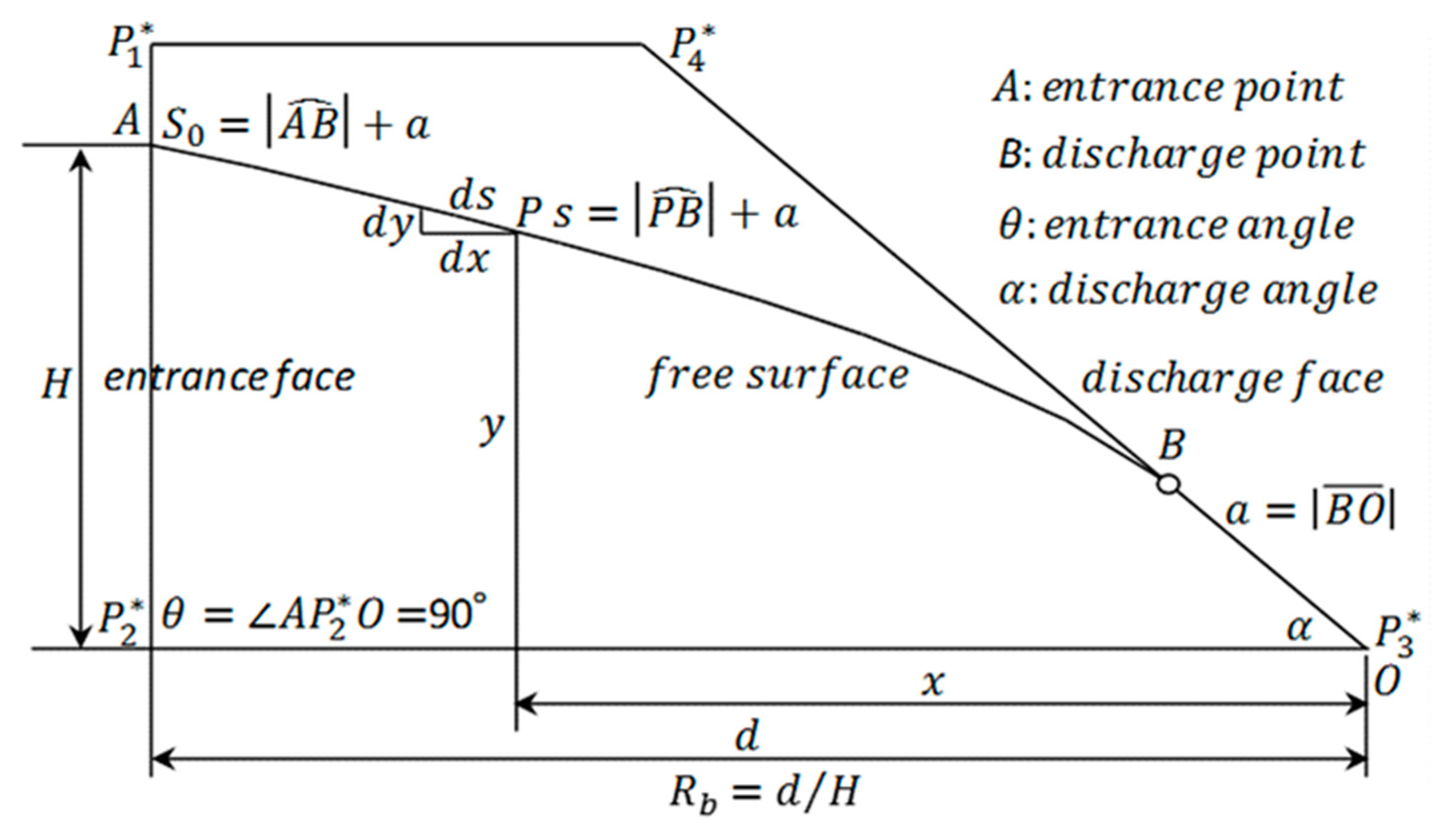
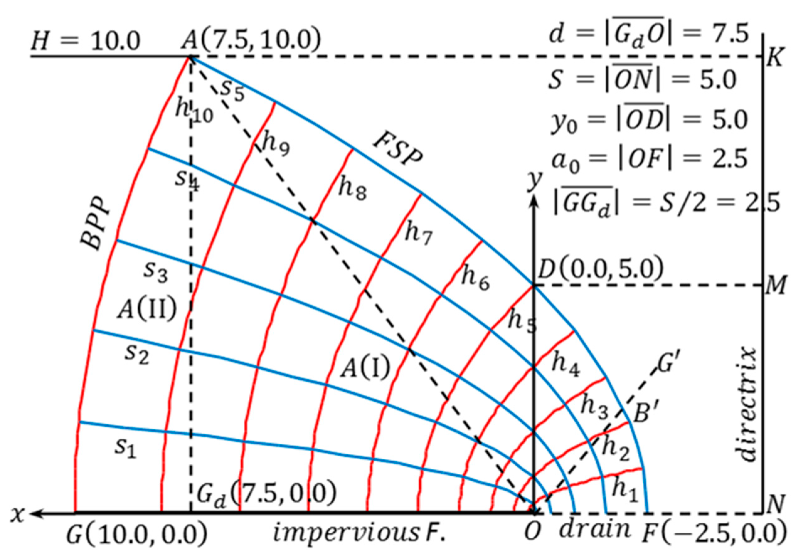
Figure 1 shows an example of the flow net of a KZ flow [5]. In this figure, $S$ is defined as follows:

$$S=\sqrt{d^2+H^2}-d$$

(5)

The free-surface parabola (FSP) of this flow is expressed in the coordinate system (i.e., KZ coordinate system) specified in Figure 1, as follows:

$$x=\frac{y^2-S^2}{2S}=\frac{y^2}{2S}-\frac{S}{2}$$

(6)

On the other hand, the boundary-potential parabola (BPP) is expressed as follows:

$$x=-\frac{1}{2\left(2d+S\right)}{y}^2+\frac{2d+S}{2}\left(\equiv \frac{y^2-F^2}{2F},F=-\left(2d+S\right)\right)$$

(7)

When $y=0$, $x=d+S/2$; therefore, $\left|\overline{G{G}_d}\right|=S/2=2.5$ in Figure 1. Both are parabolas with focus at the origin, O. The potential and stream functions in the domain are expressed by the following analytical solution [5].

$$h=\sqrt{\left(\sqrt{d^2+H^2}-d\right)\left(\sqrt{x^2+y^2}+x\right)}$$

(8)

$$s=\sqrt{\left(\sqrt{d^2+H^2}-d\right)\left(\sqrt{x^2+y^2}-x\right)}$$

(9)

In the unconfined seepage problem, it is extremely infrequent to obtain a simple theoretical solution in a finite domain using the conformal mapping method. Therefore, in order to confirm the accuracy of numerical analysis, the KZ flow is an effective numerical analysis target.

Interestingly, in the KZ flow, let us refer to the ratio, $R_b=d/H$, as the basic Ratio. Then, it is clear that two KZ flows with the same basic aspect ratio are similar. The validity of this proposition is directly confirmed by deriving the dimensionless potential, h/H from Equation (8) and the dimensionless stream function s/H from Equation (9). They become as follows:

$$h^{*}=\sqrt{\left(\sqrt{R_b^2+1}-R_b\right)\left(\sqrt{x^{*2}+y^{*2}}+x^{*}\right)}, h^{*}=h/H, x^{*}=x/H, y^{*}=y/H$$

(10)

$$s^{*}=\sqrt{\left(\sqrt{R_b^2+1}-R_b\right)\left(\sqrt{x^{*2}+y^{*2}}-x^{*}\right)}, s^{*}=s/H, x^{*}=x/H, y^{*}=y/H$$

(11)

So, if we reduce Figure 1 to 1/10, this is the KZ flow at H = 1, and the discharge also becomes 1/10. This concept of similarity is important in this paper.

The potential calculation is obtained irrespective of the permeability coefficient under the assumption of homogeneous material. In the stream function, Equation (9) must be multiplied by the permeability coefficient in order to correspond to the real discharge. However, in this paper, the result of setting the permeability coefficient $k_c=1$ is formally assumed; then, no problem occurs and the discharge of the KZ flow is expressed as $q=S=y_0$, the ordinate value of point D in Figure 1.

Equation (6) is expressed as $x=a{y}^2+c$. That is, if two independent conditions are given, this expression is determined. The KZ flow is determined by the point $A\left(d, H\right)$ and the focal point $O\left(0,0\right)$. This is described as KZ0(A, O)—the basic expression of the KZ flow. There are three other definitions of the KZ flow under the condition that point A is given: (1) the area of the KZ flow, $A_K$, is given, and this is described as KZ1(A, $A_K$); (2) the other arbitrary point $B\left(xB, yB\right)$ is given, and this is described as KZ2(A, B); (3) the discharge is given, and this is described as KZ3(A, q) where $q=S$; finally (iv) both the discharge and discharge point are given, and this is described as KZ4(q, B). For KZ1(A, $A_K$), the area of KZ flow, $A_K$, must be determined. In Figure 1, the KZ flow area is divided into two: A(I) and A(II). Using Equation (6), area A(I) is obtained as follows:

$$\mathrm{A}\left(\mathrm{I}\right)=\frac{2d+S}{2}H-\frac{H^3}{6S}$$

(12)

Using Equation (7), we have the following:

$$\mathrm{A}\left(\mathrm{II}\right)=\frac{S}{2}H-\frac{H^3}{6\left(2d+S\right)}$$

(13)

Therefore, the total area is as follows:

$$A_K\equiv \mathrm{A}\left(\mathrm{I}\right)+\mathrm{A}\left(\mathrm{II}\right)=\frac{2}{3}\sqrt{d^2+H^2}H$$

(14)

This yields the following:

$$d=\sqrt{\frac{9}{4}{\left(\frac{A_K}{H}\right)}^2-H^2}$$

(15)

Then, the focal point, $O_1$, is determined, that is, the KZ flow is determined.

For KZ2(A, B) in the KZ coordinate system, the parabola is expressed as $x=a{y}^2+c$; thereafter, the condition that points $A\left(d, H\right)$ and $B\left(xB, yB\right)$ are on the parabola determines the values of $a$ and $c$. From parabola theory, the focal point and discharge are $O_2\left(c+\left(1/4a\right),0\right) \mathrm{and} S=1/2a$, respectively.

For KZ3(A, q), $q\left(=S\right)$ is given. In the parabola $x=a{y}^2+c$, $d=a{H}^2+c$ because point A is on the parabola. The discharge $q=1/2a$ is given. Then, the parabola and focal point $O_3\left(c+\left(1/4a\right),0\right)$ are determined.

Finally, for KZ4 (q, B), in the parabola $x=a{y}^2+c$, $xB=ay{B}^2+c$ because point $B$ is on the parabola. The other description is the same as that of KZ3(A, q), and the focal point $O_4$ is determined.

All the definitions, (1), (2), (3), and (4), are simply different expressions of KZ0(A, O); however, each of them has a significant function in the equivalent KZ flow method.

In Figure 1, when the drain is inclined, such as $\overline{O{G}^{\prime }}$, the analytical solution of KZ flow becomes invalid. The free surface location moves downward as it approaches the discharge point, $B^{\prime }$, which is not on the FSP. As an approximate rule of thumb, we found that the concept of area-equivalent KZ flow is effective [5]. The deficit area, $A_{de}\left(OF{B}^{\prime }\right)$, cut by the inclined line $\overline{O{G}^{\prime }}$ is determined depending on the discharge angle, $\alpha =\angle GO{G}^{\prime }$. Let the equivalent area be defined as $A_e= A_k-A_{de}$. Then, the equivalent KZ flow having the entire area, $A_e$, is determined with point A as a fixed point. By substituting $A_e$ for $A_k$ in Equation (15), the equivalent distance, $d_e$, is determined; specifically, the equivalent origin is determined, and the area-equivalent KZ flow, KZ1($A,A_e$), is defined. In the previous study, KZ1($A,A_e$) proved to be a substantially more advantageous empirical method than A. Casagrande’s basic parabola method. However, with the goal of approximately 3% permissible error in this study, this rule of thumb must be reconsidered, especially in the range of $\alpha <90$°. 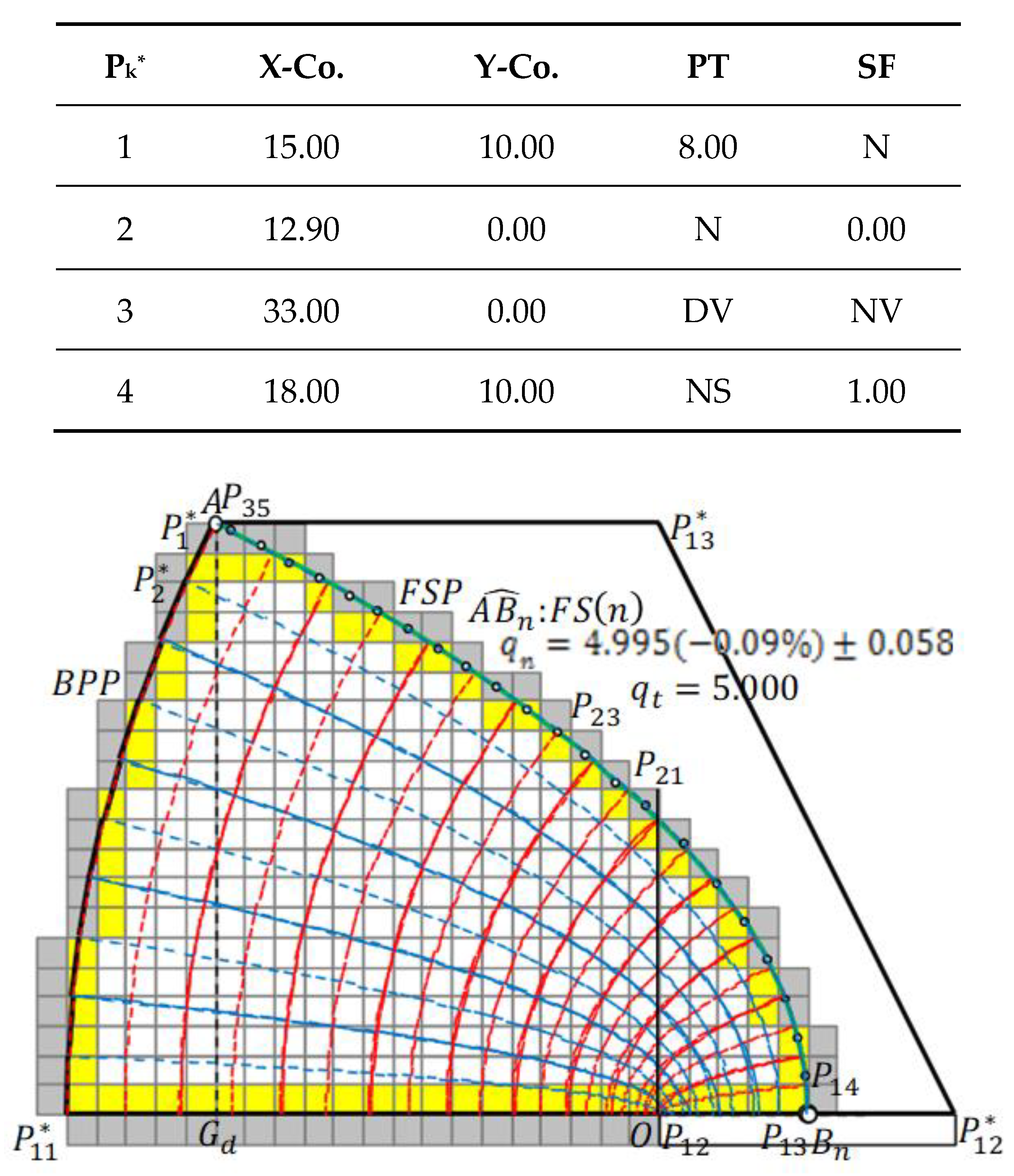Figure 2 shows the numerical calculation result of the case shown in Figure 1 (Fukuchi, 2018). Along $\widehat{P_1^{*}{P}_{11}^{*}}$, the theoretical solution of BPP is discretely given. The position coordinates of the points of $P_k^{*}, k=1, 2, \cdots ,13$ and the length of the horizontal drain are input. In the definition of $P_k, k=1,2,\cdots ,P_{35}$, $P_k=P_k^{*}, k=1, 2,\cdots ,11$ and the points $P_k,k=12,13,\cdots ,35$ are determined in the calculation process. In particular, the notation $P_k^{*}$ is used for defining the dam configuration; on the other hand, the notation $P_k$ is directly used for numerical calculation. In Figure 2, the equipotential lines are $0.1, 0.2,\cdots ,0.9H$ (division number, $N_p=10$), and the streamlines are $0.2, 0.4,\cdots ,0.8q$ (division number, $N_s=5$), indicated by solid lines. The theoretical equipotential lines are indicated by broken lines with $N_p=20$ and $N_s=10$ for streamlines. In the IFDM calculation, the active calculation elements consist of three kinds of element: normal element (colorless), near-wall element (yellow), and dummy element (gray). Numerical calculation is performed at grid points, which are centroids of each calculation element. The numerical solution agrees well with the theoretical solution. From the result of the potential calculation, the flow velocity in the horizontal direction (u) is defined at each grid point, such as $u_{i, j}=-k_c\left(h_{i+1,j}-h_{i-1,j}\right)/\left(2\Delta x\right)$. Assume that $k_c=1$. In the range of $\left|G_{d}O\right|$, 15 individual discharge values are calculated. Each discharge is calculated by the parabolic numerical integration method [1,5], then the value at either end is obtained by extrapolating the corresponding quadratic curve; this ensures sufficient accuracy. The discharge becomes $q_n=4.995\left(-0.09\%\right)\pm 0.058\left(=3\sigma \right)$; $\sigma$ is the standard deviation. Although slight dispersions of individual discharges are inevitable, the relative error of the calculated mean discharge is −0.09% with respect to the theoretical value $q_t=5.00$; this is highly accurate, being less than the 0.1% (absolute) relative error. Such features of the discharge calculation are common in the IFDM calculation.

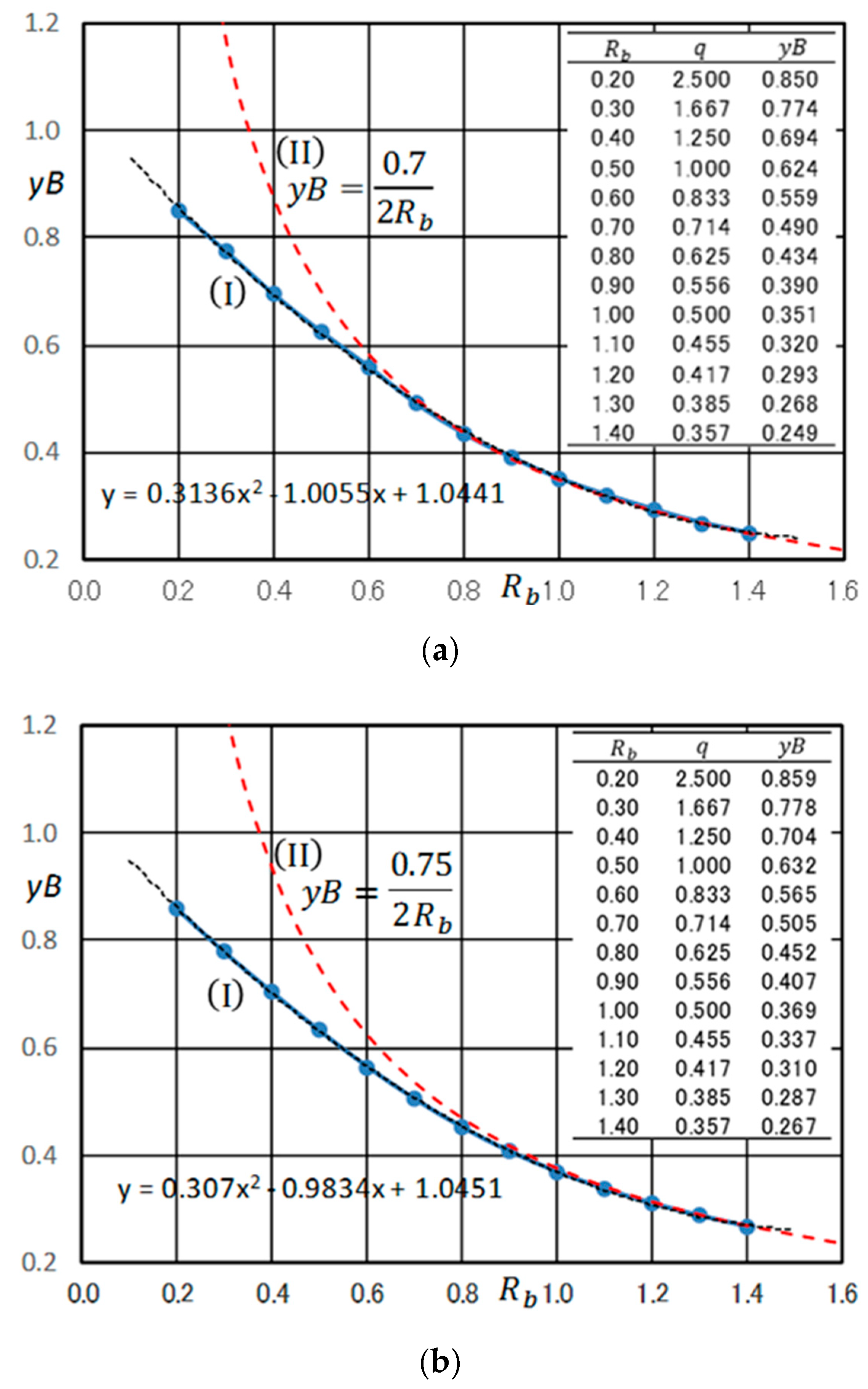
In the numerical calculation process, it is necessary to estimate the boundary points on the right side of point O. It is assumed that the curve $\widehat{P_{23}{P}_{21}{P}_{13}}$ is expressed by $x=a{y}^2+c$. This equation is derived from $P_{23}\left(x_{23},y_{23}\right)$ and $P_{21}\left(x_{21},y_{21}\right)$. Each point of $P_{20}, P_{19},\cdots ,P_{14}$ is on the curve. The y-coordinate of each boundary point is defined as $y_{21}\times (i/N), i=N-1, N-2,\cdots ,0$. Here, N = 8; the division number, N, is defined such that the calculation points are set to have appropriate intervals [5]. However, this is an example of $\mathsf{\alpha }=180°$; if $\mathsf{\alpha }\le 90°$, only one point is estimated. In this case, two equations for estimating point B are conceived: (1) linear extrapolation, $y=ax+b$ and (2) quadratic extrapolation, $y=a{x}^2+bx+c$. Generally, it makes no large difference as to which one is used; however, in the study, extrapolation is performed by (3) the KZ flow extrapolation.

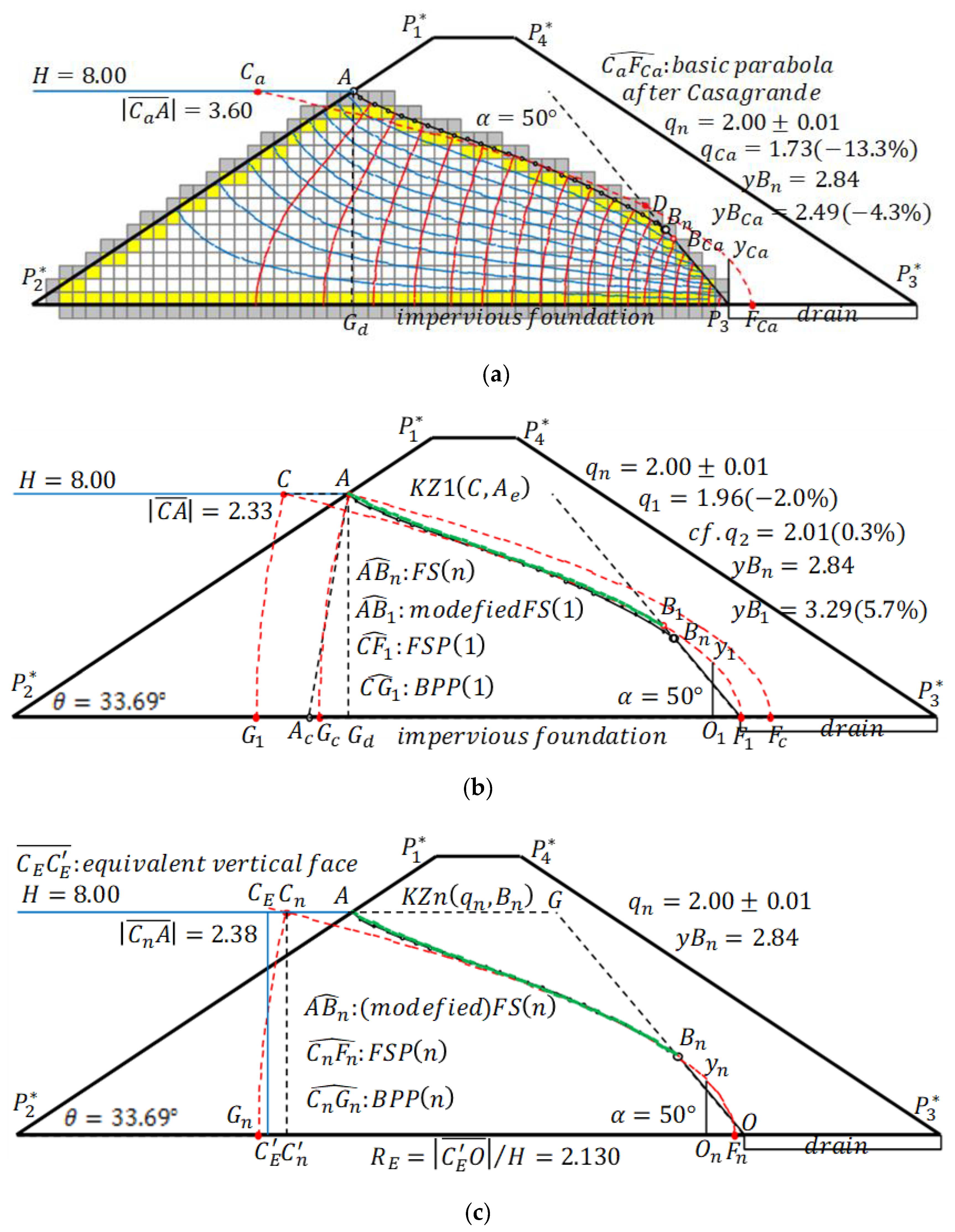
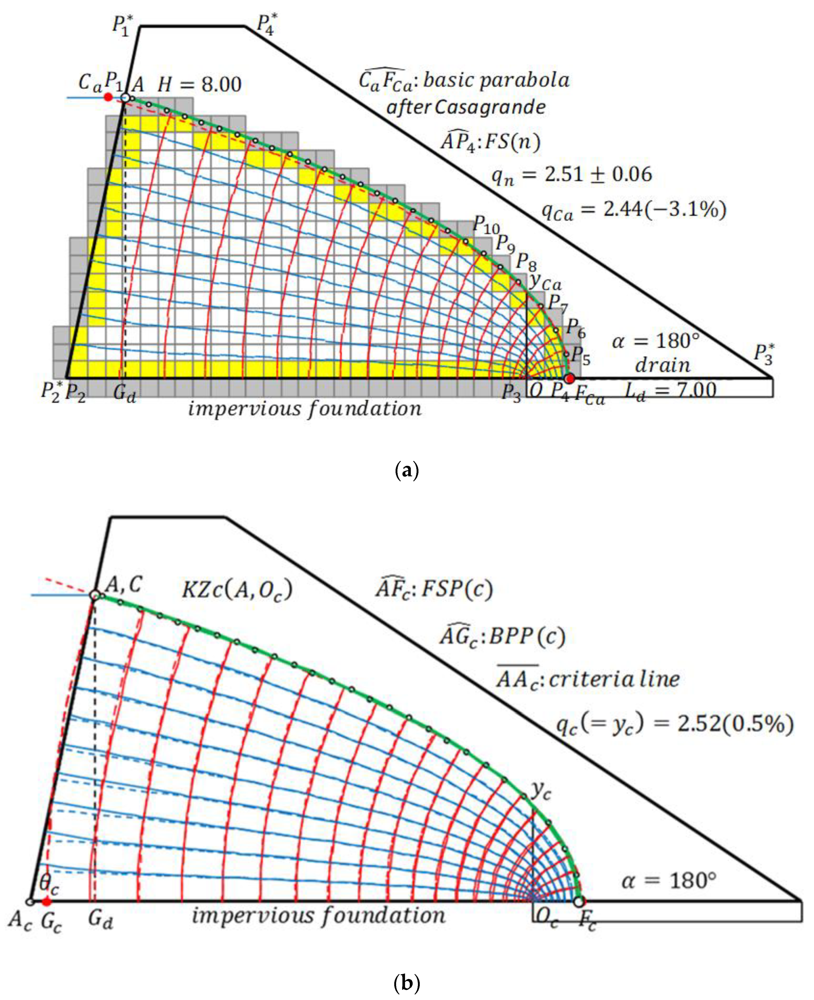
Figure 3 shows the case of a trapezoidal dam in which the entrance face is a straight line. The global coordinate values of input points and boundary conditions of the potential and stream function calculations are shown in the input data. In the potential calculation, along $\overline{P_1{P}_2}\left(\equiv \overline{A{P}_2^{*}}\right)$, the Dirichlet condition (8.00) is given; along $\overline{P_2{P}_3}\left(\equiv \overline{P_2^{*}O}\right)$, the Neumann condition (N), where the equipotential line is orthogonal to the boundary line, is given. Along $\overline{P_3{P}_4}$, the Dirichlet condition is also given; however, when the discharge angle is 90° < α < 180°, it is a position-dependent variable and is designated (DV). Along $\overline{P_{4}A}$, although the condition is the Neumann condition, it is denoted as NS to indicate that it is a free surface part. Regarding the stream function, the Neumann condition (N) is specified along $\overline{P_1{P}_2}$, and the Dirichlet condition (0.00) is designated along $\overline{P_2{P}_3}$. Along $\overline{P_3{P}_4}$, a Neumann condition orthogonal to the equipotential line is set; it is generally expressed as NV because the equipotential line at the boundary point of concern must be individually calculated according to each position. The discharge should be given as Dirichlet condition along $\overline{P_{4}A}$, but there is no problem specifying 1.00 as the Dirichlet condition. By multiplying the numerically calculated discharge, $q_n$ (as the result of the potential calculation), the correct conclusion is always obtained.

Both FSP(c) and BPP(c) are determined from the KZ flow, KZc($A,O_c$)($\equiv$KZ0($A,O$)). In Figure 3b, the point $A_c$ is given so that the areas of A(II) (Figure 1) and triangle $\mathrm{A}{A}_c{G}_d$ are equal; this practically coincides with $P_2^{*}$. Then, the entrance angle, $\theta ={\theta }_c$, is defined as the criterion entrance angle. The starting point C of FSP(c) matches point A. Moreover, the free surface of numerical calculation, FS(n), and FSP(c) coincide and the discharges would be the same. It is confirmed that the results are $q_n=2.51\pm 0.06, q_c\left(=y_c\right)=2.52 \left(0.5\%\right)$. On the other hand, in A. Casagrande’s basic parabola method, it becomes $q_{Ca}=2.44\left(-3.1\%\right)$ [5]. It is understood that his method determining point $C_a$, $\left|\overline{C_{a}A}\right|=0.3\left|\overline{P_2^{*}{G}_d}\right|$ is incorrect.

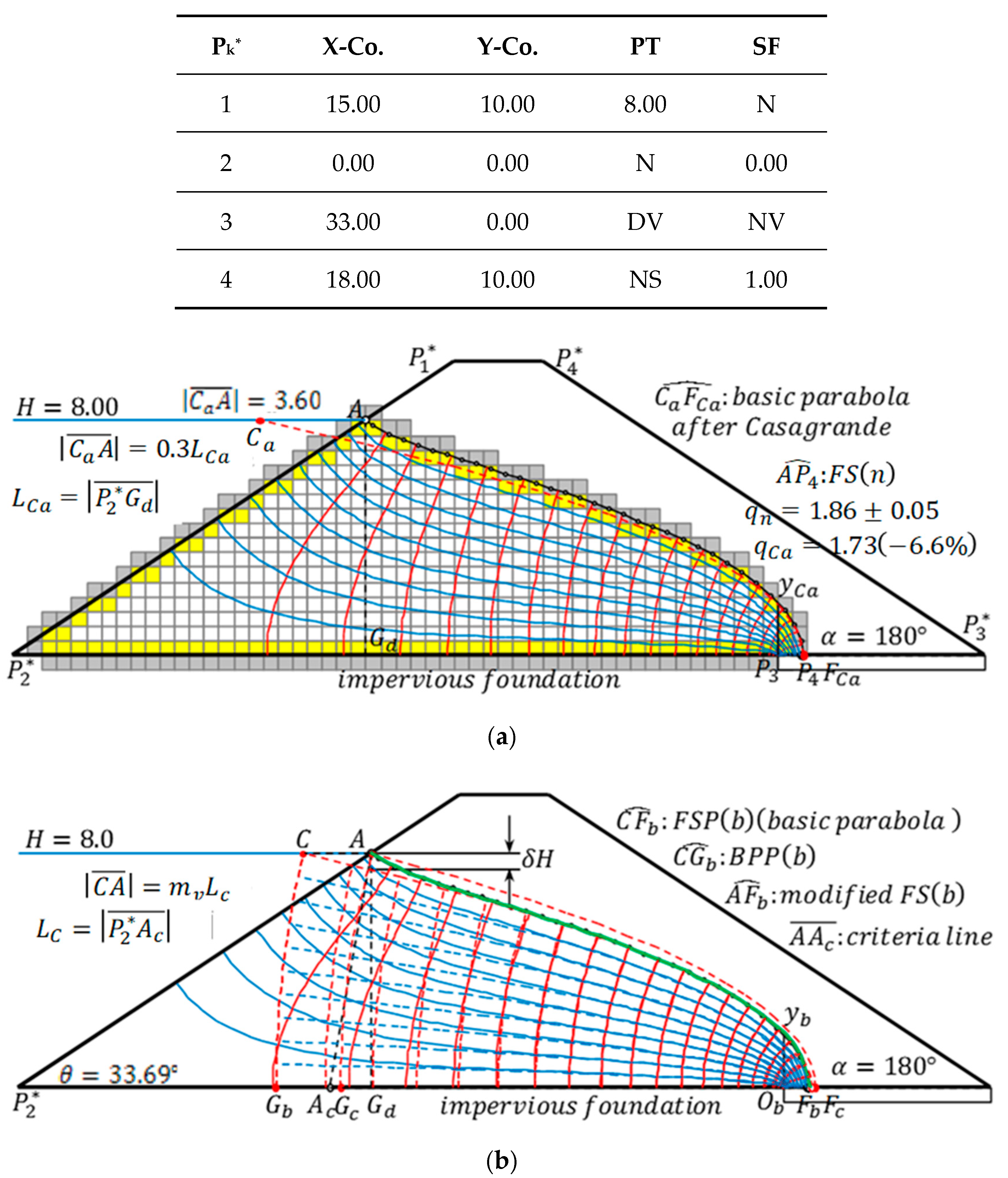
Figure 4 is a general case where point $P_2^{*}$ does not match point $A_c$; fundamental results are shown in the caption. In A. Casagrande’s method, the position of point $C_a$ is determined based on $\left|\overline{P_2^{*}{G}_d}\right|$; however, to be correct, it should be determined on the basis of $L_c=\left|\overline{P_2^{*}{A}_c}\right|$, as shown in Figure 4b. As a result of the detailed examination, in the definition $\left|\overline{CA}\right|=m_v{L}_c$, $m_v$ is determined as follows [5]:

$$m_v=0.0287R_c{}^2-0.1734R_c+0.3993, R_c=L_c/H\ge 0$$

(16)

$$m_v=0.49, R_c=L_c/H<0$$

(16a)

Therefore, point C is determined, and the basic KZ flow, KZb($C,O$), is defined. Because $q_b=1.85 \left(-0.1\%\right)$ for the numerically calculated discharge, $q_n=1.86\pm 0.05$, it can be seen that the calculation is highly accurate. (In this paper, the exact solution is defined only for the KZ flow and “rectangular dam flow” (described later). Therefore, the relative errors in the empirical methods below are evaluated by the value of the numerical calculation result.) If the entrance angle is $\theta =90°$, $R_c=L_c/H<0$, then Equation (16a) is used. Through the calculations up to this point, the discharge $q$ and discharge point $B$ were calculated. Let us define this as the empirical QB estimation. The estimation of A. Casagrande is of course an empirical QB estimation.

A remaining problem is to express accurately the free surface from FSP(b). In Figure 4b, let the deviation width of FSP(b) at point A be $\delta H$; moreover, $L=\left|\overline{G_d{B}_b}\right|$. In this case, $B_b$ matches $F_b$. Then, the deviation must be corrected between $0\le l<L$; that is, the FSP(b) must be modified to conform to the FS(n), called the modified FS(b). The modification equation is defined in the previous paper [8] as follows:

$$\delta h_{l^{*}}^{*}=\delta H{\left(\frac{1}{2}\right)}^{l^{*}/L_h^{*}}- l^{*}\delta h\left(\delta h\equiv \delta H{\left(\frac{1}{2}\right)}^{1/L_h^{*}}\right)$$

(17)

where $\delta h_{l^{*}}^{*}$ is the modification value, $l^{*}=l/L$ is the dimensionless distance, and $L_h^{*}\equiv L_h/L$ is the dimensionless half-decrease distance ($L_h$ is the half-decrease distance). In this expression, at $l^{*}=0$, it becomes $\delta h_0^{*}=\delta H$; at $l^{*}=1$, it becomes $\delta h_1^{*}=0$. The dimensionless half-decrease distance, $L_h^{*}$, generally depends on the ratio, $R_h\equiv L/H$; $L_h^{*}$ is defined as follows:

$$L_h^{*}=f\left(R_h\right)=0.5exp\left[-1.5\left(R_h-0.5\right)\right], R_h\equiv L/H$$

(18)

The detail is described in the previous paper [5]. Equation (18) is formulated based on the numerical calculation results of the rectangular dam with $R_b\ge 0.2$. It should be noted that in the case of other cross sections, some deviation may occur. In Figure 4b, it is confirmed that the green line $\widehat{A{F}_b}: modified FS\left(b\right)$ practically coincides with the calculated free surface $FS\left(n\right)$. The discharge was calculated and at the same time the free surface was defined by modifying FSP(b). Let us define this as the empirical QF estimation. The empirical QB estimation becomes the corresponding empirical QF estimation by using the modification Equation (17). The parabola FSP(b) is called the “basic parabola” in the equivalent KZ flow method as well.

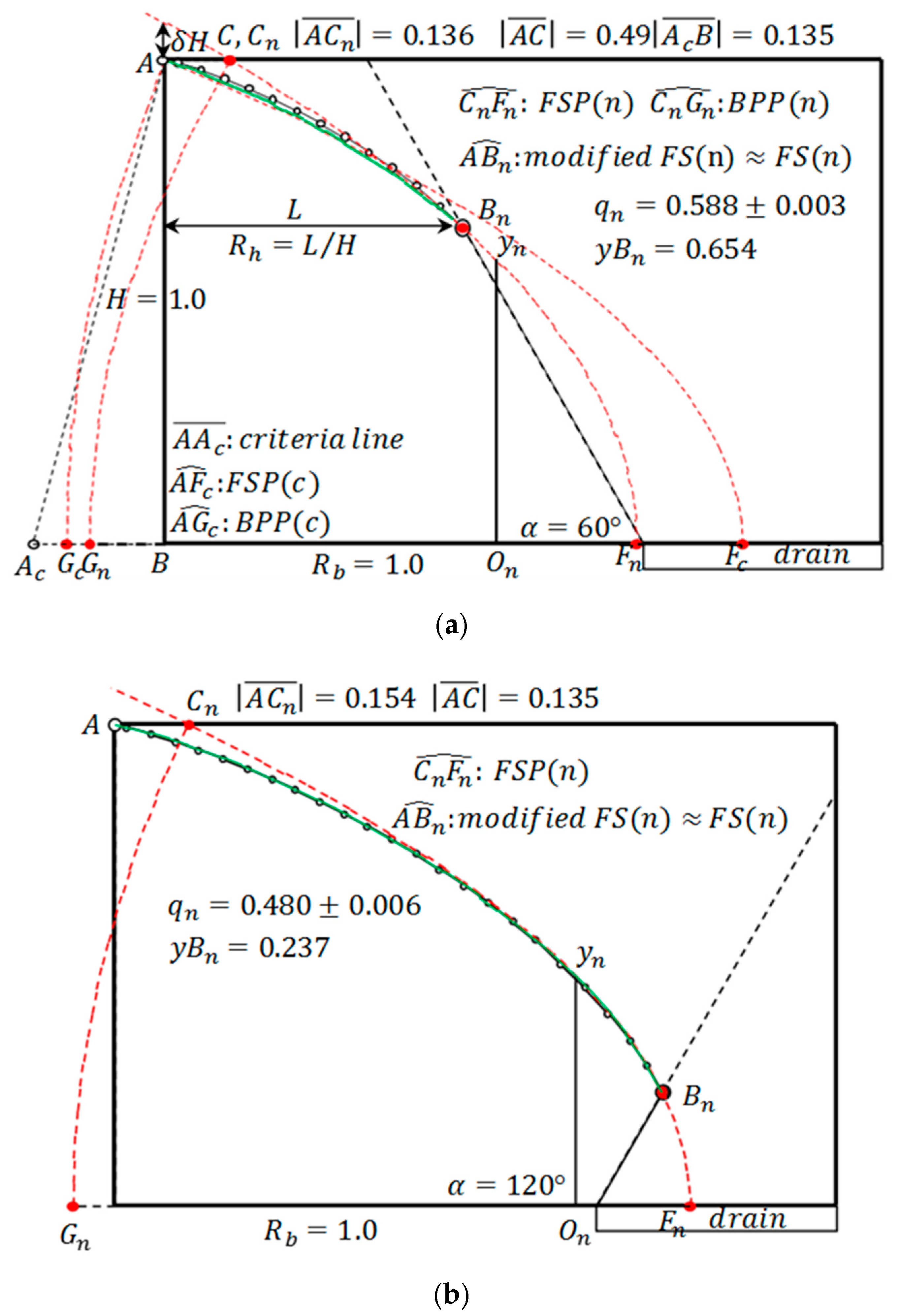
When $\mathsf{\alpha }=50°$ in Figure 4, the calculation result is shown in Figure 5. The numerical calculation yields $q_n=2.00\pm 0.01$ and $y{B}_n=2.84$. In A. Casagrande’s method, the calculation gives $q_{Ca}=1.73\left(-13.3\%\right)$ and $y{B}_{Ca}=2.49\left(-4.3\%\right)$. As $\mathsf{\alpha }$ decreases, the results given by A. Casagrande’s method rapidly deteriorate. The position of point C in Figure 5b is the same as that in Figure 4b. Using the area-equivalent KZ flow, KZ1($C,A_e$), the results are $q_1=1.96\left(-2.0\%\right)$ and $\mathrm{y}{B}_1=3.29\left(5.7\%\right)$. In terms of discharge, the result is considerably better than A. Casagrande’s method; however, as a whole, their (absolute) relative errors are too large. In the range $90°\le \mathsf{\alpha }\le 180°$, KZ1($C,A_e$) yields good results; however, as $\mathsf{\alpha }$ decreases from $90°$, it gradually yields poor conclusions [8]. Here, it should be noted that $q_2=2.01\left(0.3\%\right)$ in the discharge point-equivalent KZ flow, KZ2($C,B_n$). The position of point C varies by nature depending on the change in α; however, it can be observed that the change is practically negligible in this example.

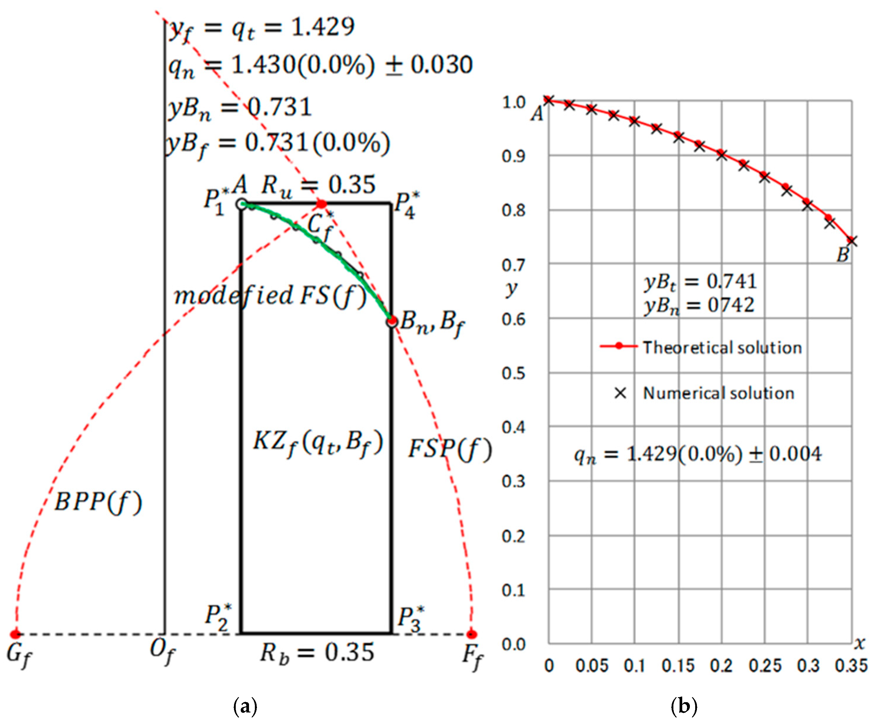
Figure 5c shows the numeric-equivalent KZ flow, KZn($q_n,B_n$). The calculated free surface FS(n) is almost precisely expressed by the modified FS(n). In the figure, the equivalent vertical face, $\overline{C_E{C}_E^{’}}$, is shown, which is set in order that the area of A(II) of KZn($q_n,B_n$) is equal to the area of the rectangle $C_E{C}_E^{\prime }{C}_n^{\prime }{C}_n$. The discharge ($q_E$) and discharge point ($y{B}_E$) of the equivalent cross section, $C_E{C}_E^{\prime }OG$, which are shown in detail later, practically coincide with those of KZn($q_n,B_n$). The numerical calculation yields the results $q_E=1.99\left(-0.7\%\right)$ and $y{B}_E=2.79\left(-0.6\%\right)$; their relative errors are both within 1%. The equivalent aspect ratio of this equivalent trapezoidal dam is $R_E=\left|\overline{C_E^{’}O}\right|/H=2.130$. The concept of equivalent aspect ratio has an important role in the following discussion.

4. Calculation Accuracy of Conventional Empirical Methods

As for the calculation accuracy of A. Casagrande’s method, because of confirming the calculation accuracy for each calculation example in the previous paper [5], it was generally found that non-negligible deviations from the numerical calculation results occur. In this paper, the methods of Schaffernak–Van Iterson and L. Casagrande regarding the seepage phenomenon of the trapezoidal dam with a vertical entrance face are discussed. These methods are included in the calculation system of A. Casagrande’s method [18]. The governing formulae and numerical calculation techniques of both these methods are shown in detail in Appendix A and Appendix B. Regarding discharge angle, the scope of the Schaffernak–Van Iterson method was set to $\alpha <30$°, and the scope of L. Casagrande’s method was set to $\alpha \le 90$°. Here, apart from such an empirical rule, the theoretical characteristics when both equations are applied to the seepage of a trapezoidal cross section $\alpha \le 90$° are considered.

In general, the discharge, $q$, and y-coordinate, $yB$, of discharge point $B$ can be expressed by the following functional definitions:

$$q=f_q\left(H,\theta ,R_b,\alpha \right)=H{f}_q\left(1,\theta ,R_b,\alpha \right)$$

(19)

$$yB=f_{yB}\left(H,\theta ,R_b,\alpha \right)=H{f}_{yB}\left(1,\theta ,R_b,\alpha \right)$$

(20)

Here, $\theta$ is the entrance angle, $R_b\left(=d/H\right)$ is the basic aspect ratio, and $\alpha$ is the discharge angle (Figure A1). These equations show the (geometrical) similarity law of seepage problems. From now on, let us set $H=1.0$. Under the conditions $\theta =90$° and $\alpha \le 90$°, let us investigate the characteristics of the calculation error when using the two types of empirical methods: the Schaffernak–Van Iterson method and L. Casagrande’s method. As already mentioned, the similarity law holds in KZ flow. This must be true for all the empirical methods as well.

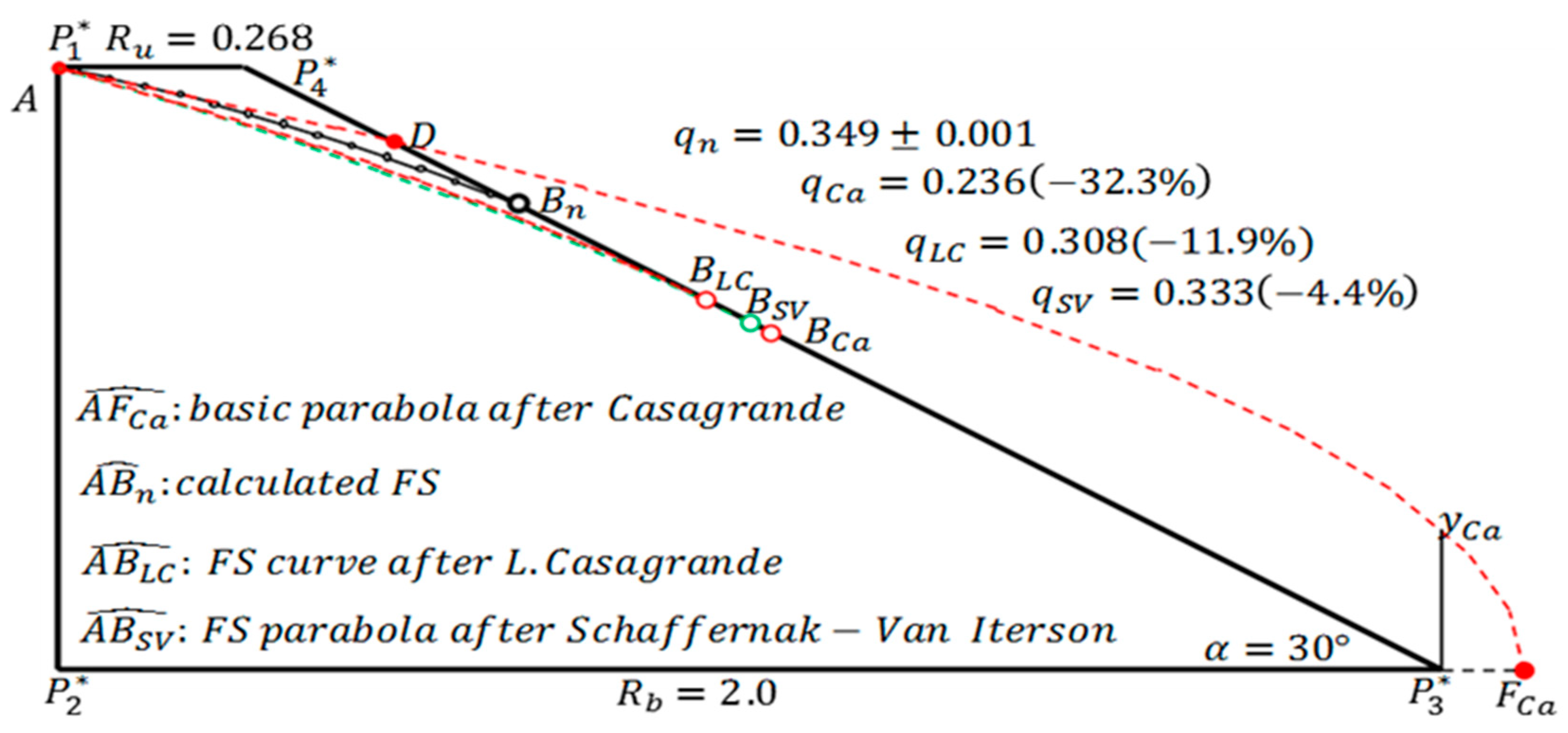
Occasionally, the overall physical phenomena image becomes distinct by considering the extreme states. Under the condition $R_b$ = 2.0, the numerical analyses are conducted, shown in Figure 6, Figure 7, Figure 8 and Figure 9, and the two extreme states of Figure 6 and Figure 9 are obtained. In Figure 7, Figure 8 and Figure 9, the calculation results using A. Casagrande’s method are also presented. 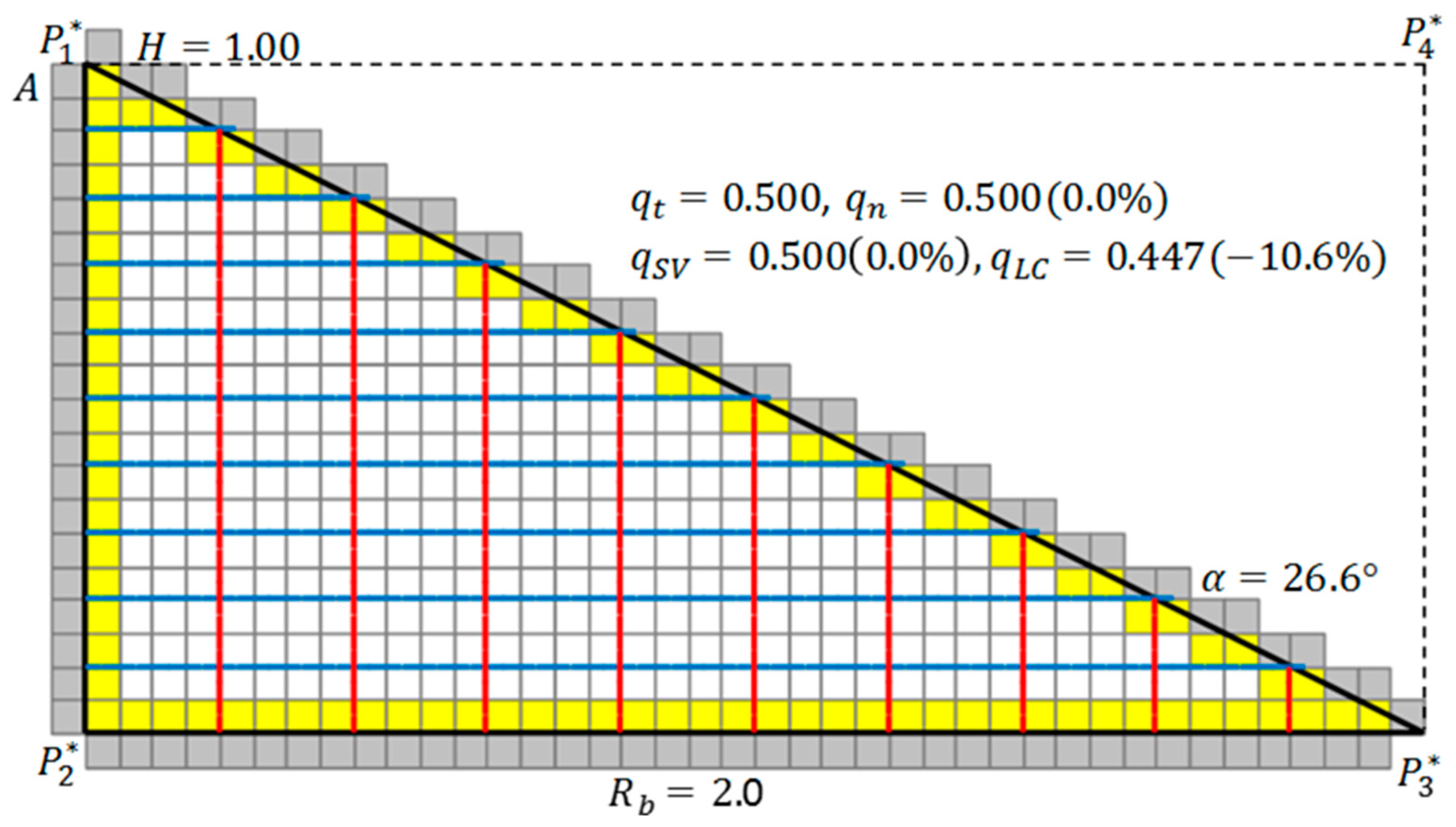Figure 6 shows the one extreme state, where the discharge angle (α) is the minimum: $\alpha ={\alpha }_{min}=\arctan \left(1/R_b\right)\cong 26.6°;$ accordingly, the entrance point (A) and discharge point (B) agree. This problem is a special confined seepage problem, and the numerically calculated discharge becomes $q_n=0.500$. In the figure, equipotential lines and streamlines are shown. The calculation area is $\mathrm{X}\left[0.0,2.0\right],\mathrm{Y}\left[0.0,1.0\right]$, and the finite difference width is $\Delta x=\Delta y=0.05$. In the calculation examples of $H=1.0$ presented in this paper, the calculation element disposition and finite difference width are always used in this specification. Except for Figure 6, illustrations of calculation element dispositions are not presented. Despite the theoretical importance of this seepage problem, no description pertaining to its analytical solution in the leading references (e.g., Polubarinova-Kochina, 1962 [19], Harr, 1991 [20]) is found. However, this problem is regarded as part of the seepage phenomenon, particularly in the case where the head of $\left|\overline{P_1{P}_2}\right|$ is 1.00 and that of $\left|\overline{P_3{P}_4}\right|$ is 0.00 in the confined seepage problem of domain $P_1{P}_2{P}_3{P}_4$; accordingly, no contradiction occurs. Therefore, its theoretical solution is $q_t=1/R_b=0.500$. Equation (A2), which is the discharge expression in the Schaffernak–Van Iterson method, would also be effective in this case. Then, this equation becomes $q_{SV}=a\sin \alpha \tan \alpha =a/a\tan \alpha =1/R_b=0.500 \left(0.0\%\right)$, which agrees with the theoretical solution. Even in L. Casagrande’s method, Equation (A12) would be an effective definition of the discharge; accordingly, $q_{LC}=a{\sin }^2\alpha =\sin \alpha =0.447\left(-10.6\%\right)$. Each method represents a one-dimensional approximation of the seepage phenomenon. The physically reasonable equation in the extreme state of Figure 6 is evidently the former expression. When $R_b\to \infty$, $q_{LC}\to q_{SV}\left(\sin \alpha \to \tan \alpha \right)$, and, generally, $q_{LC}<q_{SV}$ holds true.

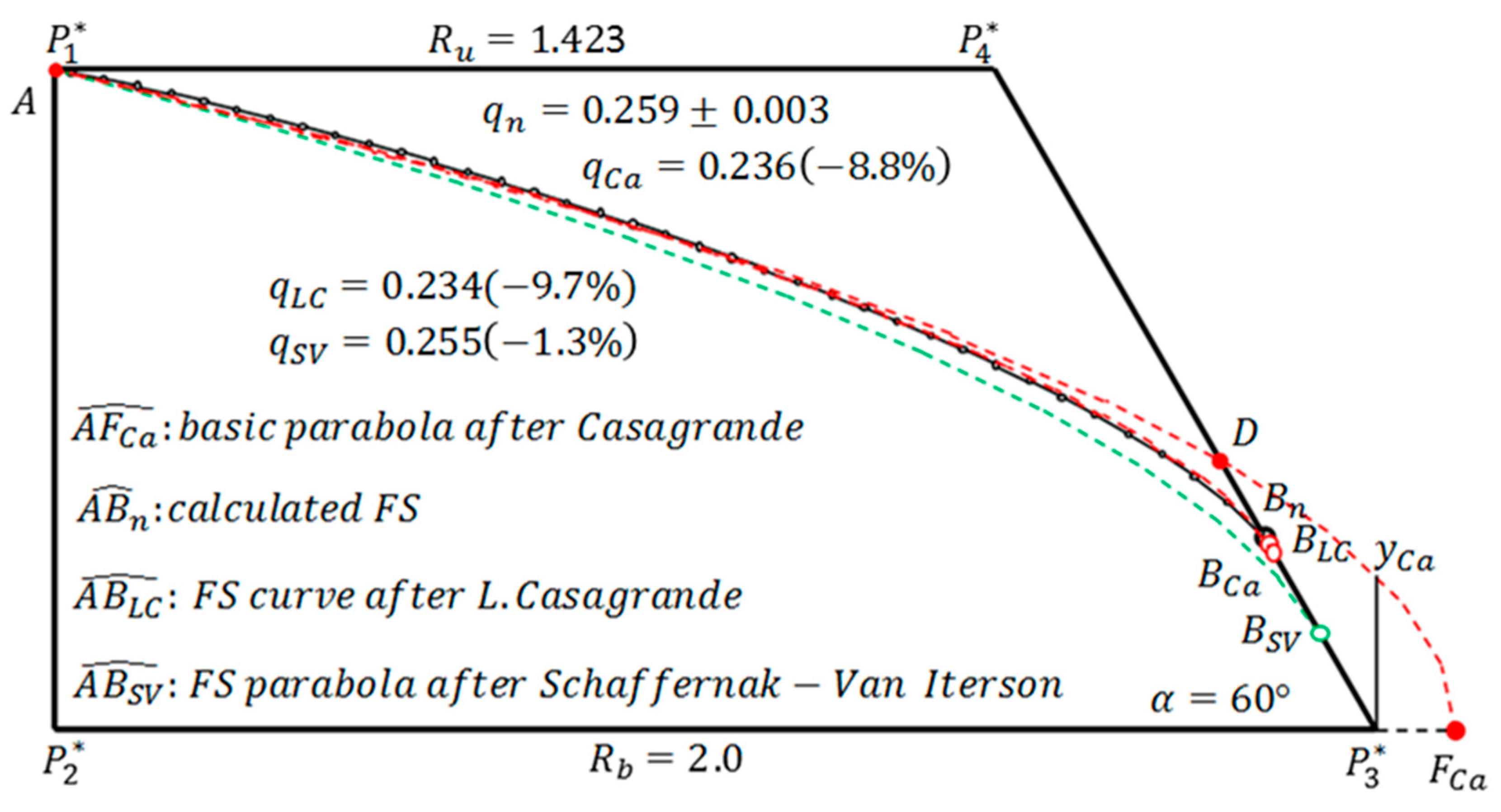
Figure 7 and Figure 8 show the results when $\alpha =30$° and $\alpha =60$°, respectively. In the figures, the values of $R_u\equiv \left|\overline{P_1^{*}{P}_4^{*}}\right|$, referred to as up-side aspect ratio, are shown. In the process of $R_u\to 0$, it has been confirmed that the discharges and discharge points from numerical calculation and empirical methods (Schaffernak–Van Iterson and L. Casagrande methods) change rapidly.

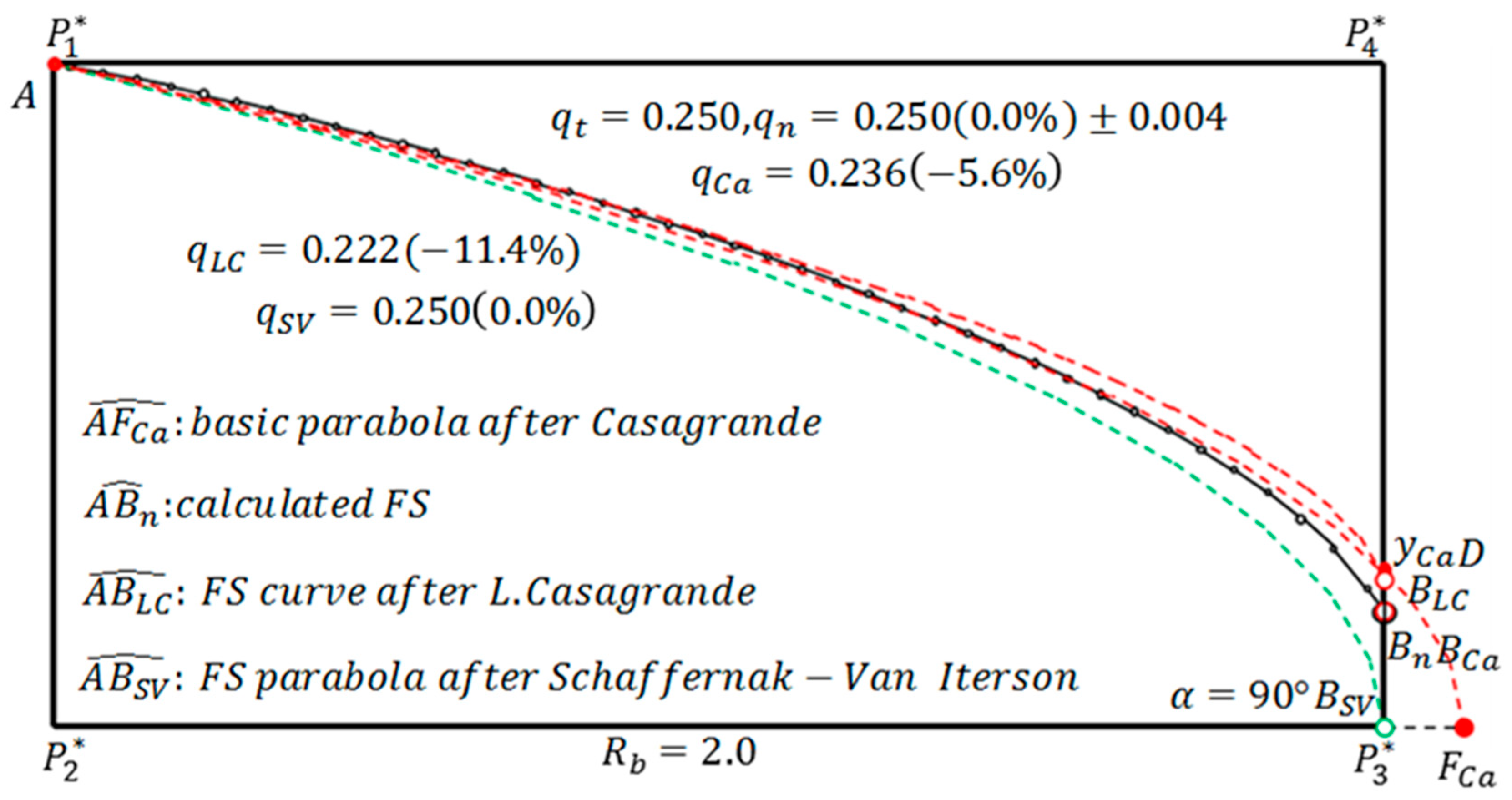
Figure 9 shows the other extreme pattern. The discharge point calculated by the Schaffernak–Van Iterson method coincides with $P_3^{*}$. The free surface distinctly deviates from the numerically calculated free surface $FS\left(n\right)$. Nevertheless, its discharge, $q_{SV}=0.250\left(0.0\%\right)$, agrees with the theoretical solution, $q_t=0.250$ (Appendix A). In this method, $q_{SV}$ is equal to the theoretical solution at both extreme states of Figure 6 and Figure 9. Even when the free surface is not correct, if a strict discharge is defined in this method, then a proper result can be obtained by the discharge-equivalent KZ flow, $\mathrm{KZ}3\left(C,q_{SV}\right)$. However, in the range ${\alpha }_{min}\ll \mathsf{\alpha }\ll 90$°, such a result is not guaranteed. In L. Casagrande’s method in Figure 9, $q_{LC}=0.222\left(-11.4\%\right)$ and the discharge point separate upward. In general, when paying attention to the free surface, the accuracy is superior to that of the Schaffernak–Van Iterson method, but the discharge error always occurs depending on $R_b$ and $\alpha$ (almost the same relative error when $\alpha ={\alpha }_{min}$). A. Casagrande (1937) [18] recommends L. Casagrande’s method as an alternative method when his basic parabola method cannot be used. However, it cannot be used from a strict viewpoint.

Table 1. Discharge calculated from empirical methods, $\theta =90°, R_b=2.0$.

(A)			(B) Discharge			(C) R.E. (%)
$\alpha (°)$	$R_u$	$q_n$	$q_{Ca}$	$q_{SV}$	$q_{LC}$	$q_{Ca}$	$q_{SV}$	$q_{LC}$
26.6	0.000	0.500		0.500	0.447	***	0.0	−10.6
30	0.268	0.350	0.236	0.333	0.308	−32.4	−4.5	−11.9
60	1.423	0.259	0.236	0.255	0.234	−8.8	−1.3	−9.7
90	2.000	0.250	0.236	0.250	0.222	−5.7	0.0	−11.5

*** A. Casagrande’s method applicable range: $30°\le \alpha \le 180°$.

and

Table 2. $yB$ -value calculated from empirical methods, $\theta =90°, R_b=2.0$.

(A)			(B) yB-Value			(C) R.E. (%)
$\alpha (°)$	$R_u$	$y{B}_n$	$y{B}_{Ca}$	$y{B}_{SV}$	$y{B}_{LC}$	$y{B}_{Ca}$	$y{B}_{SV}$	$y{B}_{LC}$
26.6	0.000	1.000	***	1.000	1.000	***	0.0	0.0
30	0.268	0.781	0.562	0.578	0.615	−21.8	−20.3	−16.6
60	1.423	0.300	0.281	0.148	0.270	−1.9	−15.2	−3.0
90	2.000	0.173	0.176	0.000	0.222	0.2	−17.4	4.8

*** A. Casagrande’s method applicable range: $30°\le \alpha \le 180°$.

summarize the results of the above empirical methods. From the viewpoint of error-within-a-few-percent estimation, none of the empirical methods shown here can be adopted. Therefore, we must establish some new empirical rules.

5. Interpolation-Equivalent KZ Flow

5.1. Creating Basic Tables

Figure 10 shows the calculation examples of ${\mathrm{R}}_{\mathrm{b}}=1.00$. In Figure 10a, when $\mathsf{\alpha }=60$°, $\left|\overline{{\mathrm{AC}}_{\mathrm{n}}}\right|=0.136$. The starting point of the parabola defined by the basic parabola of the basic KZ flow is expressed as $\left|\overline{\mathrm{AC}}\right|=0.135$ (using Equation (16a)), which is almost equal to $\left|\overline{{\mathrm{AC}}_{\mathrm{n}}}\right|$. In Figure 10b, when $\mathsf{\alpha }=120$°, $\left|\overline{{\mathrm{AC}}_{\mathrm{n}}}\right|=0.154$; moreover, it is confirmed that the location of ${\mathrm{C}}_{\mathrm{n}}$ changes depending on $\mathsf{\alpha }$. On the other hand, by definition, $\left|\overline{\mathrm{AC}}\right|$ is a quantity unique to the value of ${\mathrm{R}}_{\mathrm{b}}$ under a fixed value of $\mathsf{\theta }$, so it is the same as in Figure 10a. In Figure 10a, the modification method of FSP(n) is the same as that in Figure 4b. The only difference is that the modified value becomes negative.

Using the system adopted in Figure 10, $R_b$ and $\alpha$ are systematically changed to develop the tables for $q_n, y{B}_n$, and $C_n$. The results are listed in

Table 3. Basic table, Discharge $q_n$ depending on $R_b$ and $\mathsf{\alpha }$.

${\mathit{R}}_{\mathit{b}}$	${\mathit{\alpha }}_{\mathit{m}\mathit{i}\mathit{n}}$	${\mathit{q}}_{\mathit{m}\mathit{a}\mathit{x}}$	20	30	40	50	60	70	80	90	120	150	180
0.50	63.4	2.000						1.367	1.115	1.000	0.872	0.822	0.797
0.75	53.1	1.333					0.920	0.768	0.703	0.668	0.620	0.599	0.580
1.00	45.0	1.000				0.722	0.588	0.540	0.515	0.500	0.480	0.468	0.455
1.25	38.7	0.800				0.487	0.441	0.420	0.408	0.401	0.389	0.383	0.375
1.50	33.7	0.667			0.441	0.378	0.356	0.344	0.338	0.334	0.327	0.323	0.320
2.00	26.6	0.500		0.350	0.284	0.267	0.259	0.255	0.252	0.250	0.248	0.246	0.244
2.50	21.8	0.400		0.237	0.216	0.208	0.206	0.202	0.201	0.200	0.198	0.197	0.197
3.00	18.4	0.333	0.245	0.185	0.175	0.171	0.169	0.168	0.167	0.167	0.166	0.165	0.165
3.50	15.9	0.286	0.179	0.154	0.148	0.146	0.145	0.144	0.143	0.143	0.142	0.142	0.142
4.00	14.0	0.250	0.146	0.132	0.128	0.127	0.126	0.126	0.125	0.125	(0.125)	(0.125)	(0.125)
4.50	12.5	0.222	0.125	0.116	0.114	0.113	0.112	0.112	0.112	0.111	(0.111)	(0.111)	(0.111)

,

Table 4. Basic table, Discharge point $y{B}_n$ depending on $R_b$ and $\mathsf{\alpha }$.

${\mathit{R}}_{\mathit{b}}$	${\mathit{\alpha }}_{\mathit{m}\mathit{i}\mathit{n}}$	$\mathit{y}{\mathit{B}}_{\mathit{m}\mathit{a}\mathit{x}}$	20	30	40	50	60	70	80	90	120	150	180
0.50	63.4	1.000						0.885	0.752	0.624	0.402	0.204	0.000
0.75	53.1	1.000					0.855	0.683	0.563	0.472	0.291	0.148	0.000
1.00	45.0	1.000				0.866	0.654	0.523	0.441	0.351	0.237	0.113	0.000
1.25	38.7	1.000				0.665	0.508	0.414	0.337	0.278	0.188	0.091	0.000
1.50	33.7	1.000			0.745	0.531	0.415	0.337	0.277	0.228	0.153	0.079	0.000
2.00	26.6	1.000		0.781	0.495	0.378	0.300	0.253	0.212	0.174	0.118	0.057	0.000
2.50	21.8	1.000		0.540	0.379	0.293	0.238	0.197	0.166	0.132	0.091	0.047	0.000
3.00	18.4	1.000	0.800	0.429	0.306	0.240	0.198	0.169	0.135	0.114	0.079	0.041	0.000
3.50	15.9	1.000	0.614	0.352	0.257	0.204	0.170	0.139	0.114	0.088	0.068	0.037	0.000
4.00	14.0	1.000	0.479	0.307	0.226	0.184	0.153	0.128	0.099	0.082	(0.055)	(0.027)	(0.000)
4.50	12.5	1.000	0.414	0.277	0.201	0.162	0.142	0.115	0.089	0.066	(0.044)	(0.022)	(0.000)

and

Table 5. Basic table, starting point of FSP(n) $C_n$ depending on $R_b$ and $\mathsf{\alpha }$, shown in the value $R_b-\left|\overline{A{C}_n}\right|$.

${\mathit{R}}_{\mathit{b}}$	${\mathit{\alpha }}_{\mathit{m}\mathit{i}\mathit{n}}$	${\mathit{R}}_{\mathit{b}}-\left|\overline{\mathit{A}\mathit{C}}\right|$	20	30	40	50	60	70	80	90	120	150	180
0.50	63.4	0.298						0.402	0.327	0.306	0.253	0.229	0.209
0.75	53.1	0.587					0.640	0.596	0.585	0.582	0.569	0.560	0.576
1.00	45.0	0.865				0.900	0.864	0.863	0.860	0.869	0.846	0.861	0.880
1.25	38.7	1.135				1.130	1.135	1.137	1.146	1.151	1.130	1.139	1.148
1.50	33.7	1.401			1.393	1.396	1.400	1.409	1.414	1.419	1.406	1.403	1.399
2.00	26.6	1.923		1.910	1.920	1.925	1.931	1.929	1.931	1.936	1.923	1.928	1.919
2.50	21.8	2.437		2.431	2.437	2.442	2.444	2.446	2.444	2.453	2.451	2.451	2.453
3.00	18.4	2.947	2.932	2.942	2.950	2.952	2.950	2.947	2.959	2.954	2.932	2.959	2.952
3.50	15.9	3.454	3.430	3.454	3.458	3.458	3.457	3.456	3.460	3.466	3.451	3.447	3.443
4.00	14.0	3.960	3.930	3.959	3.961	3.960	3.959	3.960	3.969	3.967	(3.967)	(3.967)	(3.967)
4.50	12.5	4.464	4.435	4.458	4.464	4.461	4.454	4.454	4.454	4.472	(4.472)	(4.472)	(4.472)

. Figure 11a–c show the range of $R_b\le 3.50$ listed in the Tables. In Figure 11a,b, the theoretical values in the case of $\alpha ={\alpha }_{min}$ are also shown. In Figure 11c, each value of $R_b-\left|\overline{AC}\right|$ is shown by a red solid line. When $R_b=1.00 \mathrm{and} \alpha \ge 60$°, it is found that $R_b-\left|\overline{AC}\right|\cong R_b-\left|\overline{A{C}_n}\right|$. When $R_b\ge$1.25, this practically holds true regardless of α. In Figure 11c, it is noted that if $\left|\overline{A{C}_n}\right|$ is adopted instead of $-\left|\overline{A{C}_n}\right|$, the above simple relationship is not found. Parts of the parenthesized value (#. ###) listed in Table 3, Table 4 and Table 5 are those that cannot be numerically calculated under the fixed value of $\Delta x=\Delta y=0.05$ (relatively it is too large, namely, the calculation element (near-wall element) cannot be defined on the right side of point O, and calculation becomes impossible). Usually, these values may be unnecessary; however, they can be estimated from the values at $\mathsf{\alpha }=90$°. In Table 3 and Table 5, each value would be regarded as the value at $\mathsf{\alpha }=90$°. On the other hand, in Table 4, each value (#. ###) is linearly decreasing from the value at $\mathsf{\alpha }=90$° to 0 at $\mathsf{\alpha }=180$° (Figure 11b).

There is a slight discrepancy between FS(n) and modified FS(n). As previously described, Equation (18) is identified by the rectangular dam and is calculated as $L_h^{*}=0.42\cdots$. If $L_h^{*}=0.20$ is specified in Equation (17) as an individual value in this case, both of them visually match. However, in this paper, we consider this degree of deviation as an acceptable deviation.

From the information listed in Table 3, Table 4 and Table 5, the discharge, discharge point, and starting point of the FSP corresponding to any two conditions, $R_b$ and $\mathsf{\alpha }$, can be estimated using interpolation methods. There are several two-dimensional mathematical interpolation methods—the bilinear and bicubic interpolation methods (Web-Interpolation, 2017) may be fundamental. The details are described in Appendix C. In the interpolation in Table 3, Table 4 and Table 5, the bicubic interpolation method is used as a whole; however, in the range of $90°<\mathsf{\alpha } <180°$, the bilinear interpolation method would give sufficient accuracy.

By interpolation, three estimation values are obtained: discharge, $q_e$, y-coordinate value of discharge point, $y{B}_e$, and starting point, $C_e$. The discharge point, $B_e$, is defined from $y{B}_e$ and its discharge angle $\alpha$. The following five methods are conceivable as the interpolation-equivalent KZ flow methods. Under using point C, (i) KZI$\left(C, B_e\right)$, (ii) KZI$\left(C, q_e\right)$ are thought. Estimation values are $q_e, y{B}_e$, and $C_e$, then the three kinds of KZ flow can be obtained: (iii) KZI$\left(q_e,B_e\right)$, (iv) KZI$\left(C_e,B_e\right)$, and (v) KZI$\left(C_e,q_e\right)$. In the interpolation values, the value $y{B}_e$ is a key factor; therefore, in the above combinations, it is conceivable to use (i), (iii), and (iv). Here, we will confirm the results of (i) KZI$\left(C, B_e\right)$ and (iii) KZI$\left(q_e,B_e\right)$ directly for a brief description.

Figure 12a shows the results of KZn$\left(q_n, B_n\right)$ when $R_b=1.125$ and $\alpha =65$°. As for KZI$\left(q_e, B_e\right)$ and KZI$\left(C, B_e\right)$, only the calculated results are shown in the inset table of the figure to avoid the complexity of the illustration; they are within an error of 1%. Figure 12b shows the results of KZn$\left(q_n, B_n\right)$ when $R_b=1.125$ and $\alpha =135$°. The numerical results of KZI$\left(q_e, B_e\right)$ are within an error of 1%, but in the calculation of KZI$\left(C, B_e\right)$, the calculated discharge is $q_e^{*}=0.422\left(-1.5\%\right)$. In the range $R_b\ge$ 1.00, all the calculations of KZE$\left(C, B_e\right)$ almost become the error-within-a-few-percent estimation. This is because in the range, point C practically almost agrees with point $C_n$ (see Figure 11c). On the other hand, in the range $R_b\le$ 1.00 KZI estimation accuracy becomes poor. The examples of Figure 13 with $R_b=0.625$ show this fact. In Figure 13a, $\alpha =75$° and so $R_u\left(\equiv \left|\overline{AG}\right|\right)=0.357$. When $R_b$ is small and as $R_u\to 0$, both discharge and discharge point change rapidly. Therefore, the accuracy of interpolation estimation deteriorates. Figure 13b is the example of $\alpha =135$°. The result of KZI$\left(q_e,B_e\right)$ shows good accuracy. However, the calculated value of the discharge of KZI$\left(C,B_e\right)$ is $q_e^{*}=0.673\left(-6.1\%\right)$. In conclusion, in order to secure the accuracy in the case of $R_b\le$ 1.00, it is necessary to set the calculation points densely; such examples are described later.

5.2. Application Examples of Basic Tables to General Dams

Here, a usual trapezoidal dam without a drain is considered. Figure 14a shows the numeric-equivalent KZ flow, $\mathrm{KZn}\left(q_n,B_n\right)$. The method of setting the equivalent vertical face, $\overline{C_e{C}_e^{\prime }}$, is explained in Figure 5c. It is assumed that the trapezoidal cross section, $C_E{C}_E^{\prime }{P}_3^{*}G$, yields the same discharge and discharge point. However, the vertical face has to be estimated without using the numeric-equivalent KZ flow. This is expressed by using the interpolation-equivalent KZ flow, KZI$\left(C, B_e\right)$. To obtain $y{B}_e$ by the functional definition, Equation (20), it is necessary to create a three-dimensional table with the parameters $\theta ,R_b,$ and $\alpha ;$ however, this is not a promising idea because it requires many calculation points. Let $y{B}_e$ be estimated by a two-dimensional interpolation using Table 4. For this purpose, a trapezoidal cross section with a vertical entrance face corresponding to this seepage phenomenon has to be found.

In Figure 14b, first, point C of the basic parabola is located. Thereafter, $BPP\left(b\right)\left(\approx BPP\left(e\right)\right)$ and the position of $G_b\left(\approx G_e\right)$ are determined, and the corresponding equivalent vertical face, $\overline{C_E{C}_E^{\prime }}$, is defined (see Figure 5c). According to this definition, the equivalent aspect ratio becomes $R_E=\left|\overline{C_E^{\prime }{P}_3^{*}}\right|/H=2.738$. With $R_b=R_E$, $y{B}_e$ is determined by finding $y{B}_e/H$ by two-dimensional interpolation from the list in Table 4; $FSP\left(e\right)$ is determined from $\mathrm{KZI}\left(C,B_e\right)$. The numerical calculation result is $q_n=1.71\pm 0.01$ and $y{B}_n=3.50$, and $\mathrm{KZI}\left(C,B_e\right)$ yields $q_e^{*}=1.71\left(-0.01\%\right)$ and $y{B}_e=3.58\left(0.9\%\right)$. The asterisk of $q_e^{*}$ means that the value is calculated from $\mathrm{KZI}\left(C,B_e\right)$, not directly the interpolated value. The discharge of the cross section, $C_E{C}_E^{\prime }{P}_3^{*}G$, is interpolated as $q_E=1.72\left(0.5\%\right)$. In this example, under the definition of $P_3^{*}\left(45.00, 0.00\right)\left(\alpha =20.3°\right)$, it yields $q_n=1.18\pm 0.01, y{B}_n=3.82,$ and $q_e^{*}=1.18\left(-0.1\%\right), y{B}_e=3.79\left(-0.3\%\right)$; these results have sufficient accuracy.

Figure 15 shows an example of another interpolation-equivalent KZ flow, KZI$\left(C,B_e\right)$, which corresponds to Figure 5. A precise conclusion, $q_e^{*}=2.01\left(0.4\%\right)$ and $y{B}_e=2.82\left(-0.1\%\right)$, is obtained. Many other cases were examined for KZI$\left(C,B_e\right)$. Concerning the discharge angle, the applicable range is $20°\le \alpha <180$°, and regarding the entrance angle, the applicable range is $20°\le \theta \le 90$°. However, the equivalent aspect ratio, $R_E$, must be smaller than 4.5 (Table 3, Table 4 and Table 5).

By the above formulation, it seems that the target of error-within-a-few-percent estimation has practically been reached. However, the combination of $\theta$ and $\alpha$ where $R_b$ and $R_u$ $\left(R_b\ge R_u\right)$ are exceedingly small must be eliminated.

5.3. Special Cases When the Basic Table Cannot Be Used

When the up-side aspect ratio, $R_u$, is small in the trapezoidal dam with a vertical entrance face, the calculation accuracy is poor, as shown in Figure 13a. To improve this, a table for $q_n$ and $y{B}_n$ is developed by systematically changing $R_u$ and $R_b$; the results are listed in

Table 6. Trapezoidal dam with $\mathsf{\theta }=90$°, and small value of $R_u$, discharge $q_n$ depending on $R_u$ and $R_b$.

${\mathit{R}}_{\mathit{u}}\downarrow ,{\mathit{R}}_{\mathit{b}}\to$	0.20	0.30	0.40	0.50	0.60	0.70	0.80	0.90	1.00
0.20	2.500	1.871	1.501	1.255	1.078	0.945	0.842	0.759	0.691
0.30	(2.201)	1.667	1.350	1.136	0.981	0.862	0.770	0.696	0.634
0.40	***	(1.539)	1.250	1.055	0.914	0.806	0.721	0.652	0.595
0.50	***	***	(1.183)	1.000	0.867	0.766	0.686	0.621	0.567

and

Table 7. Trapezoidal dam with $\mathsf{\theta }=90$°, and small value of $R_u$, discharge point $y{B}_n$ depending on $R_u$ and $R_b$.

${\mathit{R}}_{\mathit{u}}\downarrow ,{\mathit{R}}_{\mathit{b}}\to$	0.20	0.30	0.40	0.50	0.60	0.70	0.80	0.90	1.00
0.20	0.850	0.849	0.841	0.838	0.833	0.832	0.832	0.831	0.831
0.30	(0.798)	0.774	0.764	0.759	0.754	0.752	0.748	0.747	0.743
0.40	***	(0.723)	0.694	0.682	0.679	0.676	0.674	0.672	0.670
0.50	***	***	(0.646)	0.624	0.622	0.611	0.612	0.608	0.602

. Because the defined interval is small, bilinear interpolation can be used (Appendix C). The tables are utilized for analyzing the case of $R_b\ge R_u$; however, for the continuous analysis with $R_u\ge$ 0.20, the values in parentheses ($R_b<R_u$) are also prepared by numerical calculation. Figure 16 shows a calculation example. In the defined region of the tables, KZI$\left(q_e, B_e\right)$ ensures that the error-within-one-percent estimation is achieved.

Next, when focusing on and analyzing the center core part of an earth dam, dedicated tables are also prepared. The cross section is bilaterally symmetric. The results are summarized in

Table 8. Dam center core, discharge $q_n$ depending on $R_u$ and $R_d$.

${\mathit{R}}_{\mathit{u}}\downarrow ,{\mathit{R}}_{\mathit{d}}\to$	0.20	0.30	0.40	0.50	0.60	0.70	0.80	0.90	1.00	1.20	1.40
0.20	2.500	1.886	1.526	1.287	1.115	0.986	0.885	0.803	0.737	0.632	0.557
0.30	(2.175)	1.667	1.367	1.163	1.013	0.901	0.812	0.740	0.681	0.589	0.522
0.40	***	(1.515)	1.250	1.071	0.938	0.837	0.757	0.692	0.639	0.555	0.493
0.50	***	***	(1.166)	1.000	0.882	0.788	0.715	0.654	0.605	0.527	0.469

and

Table 9. Dam center core, discharge point $y{B}_n$ depending on $R_u$ and $R_d$.

${\mathit{R}}_{\mathit{u}}\downarrow ,{\mathit{R}}_{\mathit{d}}\to$	0.20	0.30	0.40	0.50	0.60	0.70	0.80	0.90	1.00	1.20	1.40
0.20	0.850	0.840	0.835	0.815	0.802	0.792	0.787	0.760	0.751	0.729	0.692
0.30	(0.777)	0.774	0.766	0.757	0.724	0.716	0.707	0.676	0.669	0.634	0.601
0.40	***	(0.706)	0.694	0.686	0.653	0.645	0.641	0.610	0.603	0.568	0.545
0.50	***	***	(0.666)	0.624	0.616	0.580	0.574	0.550	0.543	0.519	0.496

. In this case, the down-side aspect ratio is defined as $R_d\equiv \left|\overline{P_2^{*}{P}_3^{*}}\right|$. The table is intended for analyzing the result in the case of $R_d\ge R_u$; however, for the continuous analysis with $R_u\ge$ 0.20, the values in parentheses ($R_d<R_u$) are also prepared. Figure 17 shows a calculation example. The bilinear interpolation is used as well. Using the defined region of the tables, KZI$\left(q_e, B_e\right)$ almost ensures that the error-within-one-percent estimation is achieved.

There may be other particular cases to be investigated. For example, the problems pertaining to inclined dam cores and dams with an entrance angle of $\theta >90$° have not yet been considered. However, in these cases, it has been confirmed that the numeric-equivalent KZ flow, KZn ($q_n,B_n$), is effective as well. In such cases, if necessary, two-dimensional tables for obtaining the interpolation-equivalent KZ flow could also be prepared.

5.4. Theoretical Consideration on the Seepage of Rectangular Dams

Finally, we will consider a rectangular dam where $R_b=R_u$. Figure 18a shows how $yB$ of the rectangular dam changes depending on $R_b$. The regression Equation (21) is as follows [5]:

$$yB=f\left(R_b\right)=0.3136R_b^2-1.0055R_b+1.0441$$

(21)

The theoretical discharge is $q_t=H^2/\left(2d\right)=1/\left(2R_b\right)$ [19]. Let the discharge point defined by Equation (21) be $B_f$. Then, the equivalent KZ flow is defined by $K{Z}_f\left(q_t, B_f\right)$. Figure 19a shows that the result of the numerical calculation and the result of $K{Z}_f\left(q_t, B_f\right)$ agree with high accuracy. Modified FS(f) calculated from FSP(f) by Equations (17) and (18) also almost agrees with the free surface FS (n) obtained by numerical calculation.

It is clear that Equation (21) is a quadratic equation and has an application limit. In the case of $R_b>1.4$, the calculation is conducted by using the interpolation-equivalent KZ flow, KZI$\left(C, B_e\right)$, based on Table 4; however, there is a convenient method specifically used for rectangular dams. Figure 20a shows the relationship between $yB$ and $q$ in the same data as that shown in Figure 18a. It is certain that as $R_b\to \infty$, $\left(q, yB\right)\to \left(0,0\right)$. As $R_b=1.4$, $\left(q, yB\right)=\left(0.357,0.249\right)$. The linear equation passing through these two points is as follows.

$$yB=0.6975q\cong 0.7q$$

(22)

This seems to hold in the range $0.8\le R_b$. Now, $q=q_t=H^2/\left(2d\right)=1/\left(2R_b\right)$, therefore

$$yB=0.7/\left(2R_b\right)$$

(23)

This equation is shown in Figure 18a, (II). Although the ranges of Equations (21) and (23) overlap, let us set the application range of Equation (21) as $R_b<1.0$ and that of Equation (23) as $R_b\ge 1.0$ for convenience.

Here, the condition that the seepage phenomenon in the vicinity of the discharge point becomes independent of the shape of the entrance face is considered. As shown in Figure 4b, the theoretical solution of the basic KZ flow, KZb$\left(C, O_b\right)$, and that of the numerical calculation are different as a whole; however, near the discharge point, the two are practically the same. This indicates that when $R_b$ is increased to some extent, the flow near the discharge point is independent of the shape of the entrance face. This is an example of the case $\mathsf{\alpha }=180$°; nevertheless, the concept seems to hold for any value of α. Let this concept be called “discharge-independent principle”. Figure 20a implies that the above concept holds even at α = 90°. Theoretically, it is presumed that Equation (23) is the asymptotic line of the function $yB=f\left(q\right)$ as $R_b\to \infty \left(q\to 0\right)$. It may be considered that a discharge point specific to the discharge is defined in the range $R_b\ge$ 1.0.

The accuracy of numerical calculation depends on the difference width. In this paper, as H = 1.00 is designated, ∆x = ∆y = 0.05 is used for all numerical calculations. As using $\Delta x=\Delta y=0.025$, the result is $q_n=1.429\left(0.0\%\right)+0.004$, and $y{B}_n=0.742$. There is almost no difference in the discharge compared to the former, but the position of the discharge point is calculated slightly higher. The theoretical solution for the free surface of a rectangular dam was derived by Polubarinova-Kochina [19]. In quantifying the theoretical solution, a systematic iterative calculation is required, which was detailed in the previous paper [4]. Figure 19b shows the comparison between the numerical solution and the theoretical solution. It is observed that the agreement is almost good. It is thought that all of the results in Figure 18a will be slightly different if ∆x = ∆y = 0.025 is used. Note that the theoretical solution only gives the free surface, but it requires much more calculation time than the numerical calculation of IFDM.

Finally, let us consider the case of 90° $<\mathsf{\alpha }<180$°. Figure 21 shows the relationship between $yB$ and $q$ depending on $\mathsf{\alpha }$:$yB=f_{\alpha }\left(q\right)$ obtained from Table 3 and Table 4. It is shown in the range $0.5\le R_b\le 3.5$. We have already described the case of α = 90°, here the line of Equation (22), $yB=\beta q \left(\beta =0.7\right)$, is also shown. Corresponding to 90° $<\mathsf{\alpha }<180$°, it is thought to be $0.7>\mathsf{\beta }>0$. At $\mathsf{\alpha }=180$°, $yB=0$, but at discharge point $\left(xB,yB\right)$, $xB=0.5q$, so the discharge point is uniquely determined, see Figure 1. Now, suppose the following relationship holds.

In order to confirm the numerical calculation accuracy, we will examine how the above discussion regarding the rectangular dam changes when theoretical solutions are used for both q and yB. Figure 18a is changed to Figure 18b. Figure 20a is changed to Figure 20b. There is no change in the theoretical formation, but there is a 1–2% difference in the calculation of yB. In the numerical calculation, the discharge calculation error remains within 1%, may be around 0.1%. However, the error of yB changes depending on the calculation conditions, especially the difference width. Higher-accuracy numerical calculation is possible if necessary, but it is considered that the numerical calculations performed in this paper have sufficient accuracy from an engineering point of view.

$$\beta =0.7(180°-\alpha )/90°$$

(24)

In Figure 21, the line $yB=\beta q$ is shown regarding $\mathsf{\alpha }=120$° and $\mathsf{\alpha }=150$°. Although there is a slight discrepancy in numerical calculations, Equation (24) seems to be valid. This indicates that under the conditions of 90° $<\mathsf{\alpha }<180$° and $R_b\ge 1.0$, the discharge point is uniquely determined corresponding to $q$ and $\mathsf{\alpha }$. In the range $\mathsf{\alpha }<90$°, it is easily confirmed that Equation (24) does not hold. In such a case, the discharge independent principle still may hold. This is a problem to be solved in the future.

5.5. Summary of This Section

This section details the new empirical method. In order to provide the benefits of applying this method to the field, the whole picture is summarized in a compact manner. As expressed by Equations (19) and (20), the shape determinant of the isotropic seepage phenomenon of earth dam is $\left(H,\theta ,R_b,\alpha \right)$. However, by applying the similarity law of seepage phenomenon, it is reduced to $\left(1,\theta ,R_b,\alpha \right)$. Furthermore, by replacing the dam of arbitrary shape with an equivalent vertical-entrance-face trapezoidal dam, it is reduced to $\left(1,90°,R_b,\alpha \right)$. The basic process is as follows: (i) To replace a general dam with an equivalent vertical-entrance-face trapezoidal dam, determine the starting point C of the basic parabola by Equation (16), (ii) Furthermore, the position of the vertical entrance face is determined in consideration of Equation (13) (see Figure 14 and Figure 15). Now we are ready to use Basic Table 4, (iii) The discharge point $B_e$ is determined by Table 4 owing to applying the similarity law, then the empirical QF estimation is completed by KZI(C, $B_e$).

In order to execute the above calculation precisely, it is necessary to create a dedicated system. However, a rougher approach would be acceptable to approximately know the discharge and the discharge point. In this paper, the bicubic interpolation method is used in the interpolation of the basic table, but the results are not so different even in the bilinear interpolation.

This empirical method using the basic Table 4 has a wide applicable range: $R_b>1.0$, $20°\le \alpha <180°$, and $20°\le \theta \le 90°$. Regarding the three exceptional cases where sufficient accuracy is not ensured by the above method, (i) vertical-entrance-face trapezoidal dam with small upper side, (ii) symmetrical dam center core, and (iii) narrow rectangular dam, dedicated tables were created individually. By creating Table 6, Table 7, Table 8 and Table 9 and the insert table of Figure 18, the approximate values of discharge and discharge point can be instantaneously grasped.

Interestingly, the actual soil material is generally anisotropic. In this case, the governing equation of the seepage phenomenon is often expressed by the following equation.

$$k_x\frac{{\partial }^{2}h}{\partial x^2}+k_y\frac{{\partial }^{2}h}{\partial y^2}=0 \left(or\frac{{\partial }^{2}h}{\partial x^2}+\left(k_y/k_x\right)\frac{{\partial }^{2}h}{\partial y^2}\right)$$

(25)

$k_x$ is the permeability coefficient in the x direction and $k_y$ is the permeability coefficient in the y direction. In this case, the flow net is created geometrically or by numerical calculation from the flow net created assuming isotropy (Harr, 1991, p. 29 [20]). For this reason, the empirical method proposed in this paper is also applied to such anisotropic seepage dams.

6. Conclusions and Discussion

In the previous paper [8], the concept of the equivalent KZ flow method was formulated. In this study, this method is developed as a more accurate empirical method. The contents of this paper are summarized as follows.

Conventionally, there were three empirical methods stipulated in the design standards regarding the seepage of earth dam: (i) A. Casagrande’s method, (ii) the Schaffernak–Van Iterson method, and (iii) L. Casagrande’s method. Theoretical consideration on the method (i) and the evaluation of the error were shown in the previous paper. In this paper, the methods (ii) and (iii) are newly considered and the characteristics of the calculation error are confirmed. The investigations revealed that it is impossible to stably use these methods even if the permissible error is set to 10%. It is clear that the conventional methods essentially need to be reviewed in order to reach the accuracy within a few-percent error in a wide range.

For the natural development of the logic from the previous paper [5] to the present paper, the basic conclusions of the concept of the equivalent KZ flow method presented in the previous paper were briefly summarized. The area-equivalent KZ flow, KZ1$\left(C, A_e\right)$, is an important method reached in the previous paper. This method powerfully rebuts the basic parabola method of A. Casagrande. This method obtains good results in the range of $90°\le \alpha \le 180°$, but in the range of $\alpha <90°$, there is a drawback that the accuracy becomes worse as $\alpha$ becomes smaller. In order to overcome this difficulty, the concept of the numeric-equivalent KZ flow, $\mathrm{KZn}\left(q_n,B_n\right)$, is important among the several equivalent KZ flows proposed in the previous paper. By using this KZ flow, the free surface shape that fits the numerical calculation can be calculated almost accurately in any shape of trapezoidal dam. A. Casagrande’s method estimates the discharge and discharge point, but no method for accurately estimating the free surface has been proposed. This is defined as empirical QB estimation. On the other hand, in the numeric-equivalent KZ flow, the free surface itself can be estimated by modifying the corresponding free surface parabola FSP(n) using a modification equation. This is defined as empirical QF estimation. All of the equivalent KZ flow methods in this paper give the empirical QF estimation.

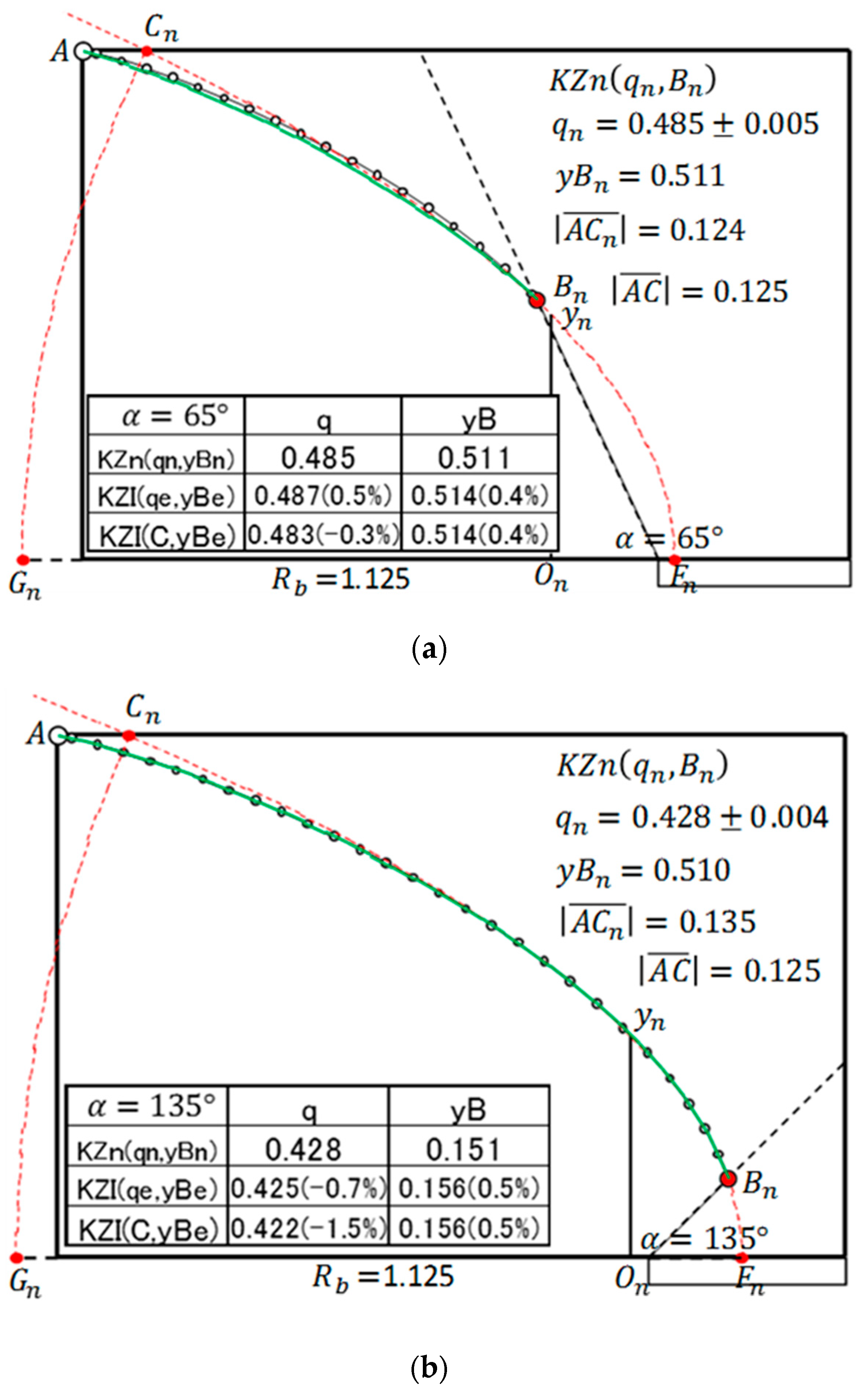
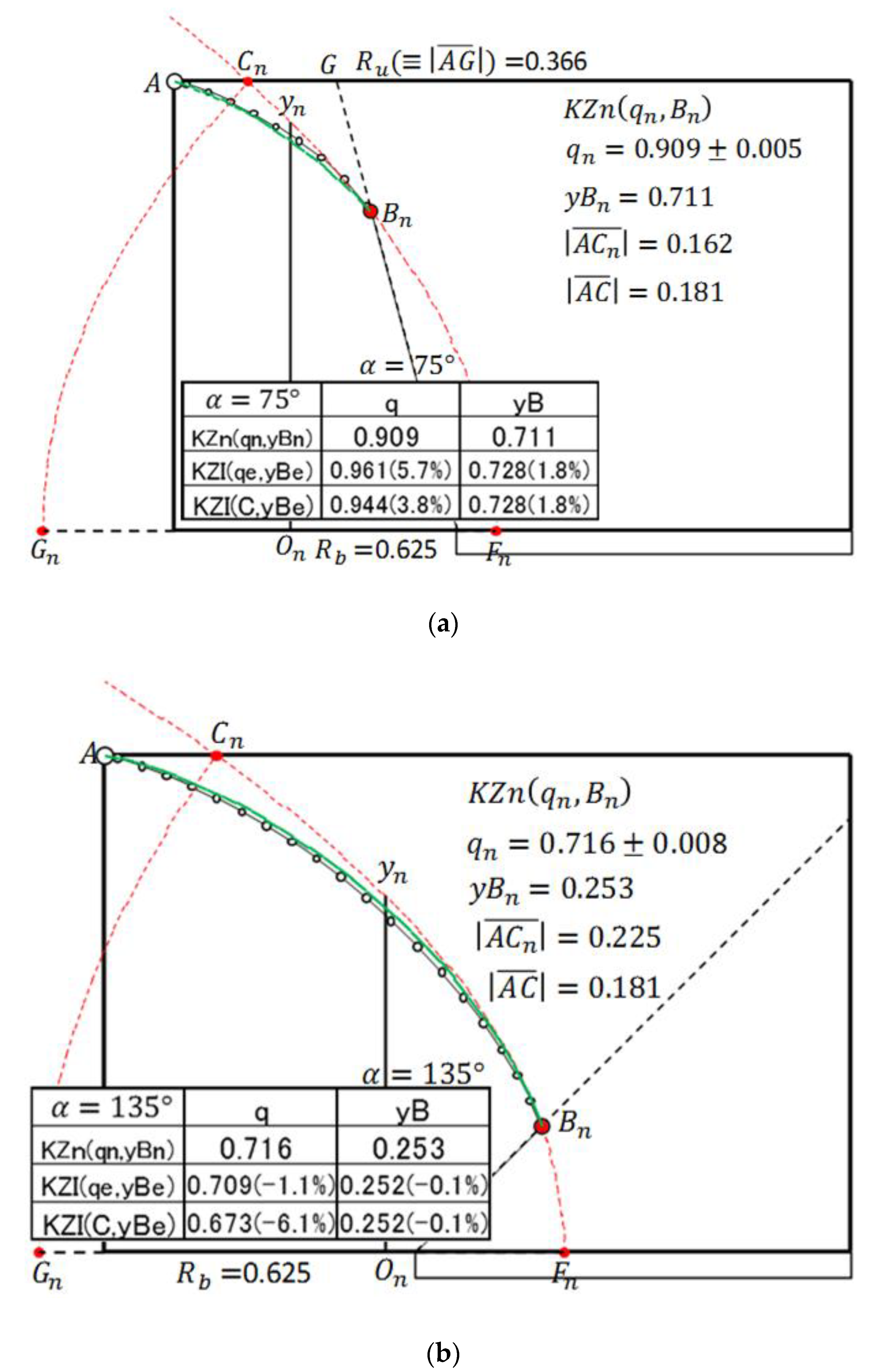
A set of the determinant factors of the seepage of a trapezoidal dam is $\left(H,\theta ,R_b,\alpha \right)$, but it became clear that only the case of $H=1.00$ should be considered due to the similarity law of seepage. Therefore, in order to determine the values of $q$ and $yB$ by interpolation method, it is sufficient to create a three-dimensional “Table” of $\left(\theta ,R_b,\alpha \right)$. It is possible in principle but inconvenient. In this paper, a two-dimensional table is created by fixing $\theta =90°$. As long as $\theta =90°$, the interpolation is completed, and if the estimated values are $q_e$ and $y{B}_e$, the corresponding interpolation-equivalent KZ flow, KZI($q_e, B_e)$, is obtained. However, in the case of $\theta <90°$, an empirical method must be devised separately. A. Casagrande proposed a method to determine the starting point of the basic parabola$C_a$. The starting point changes depending on all the factors of $\theta ,R_b,$ and $\alpha$, but he defines the basic parabola drawn when $\alpha =180°$ and even if $\alpha$ changed, he considered the starting point immutable. The author basically adopted his hypothesis (in this sense, the author’s idea is basically dependent on A. Casagrande’s method) but with a more rational method for determining the starting point $C$ of the basic parabola.

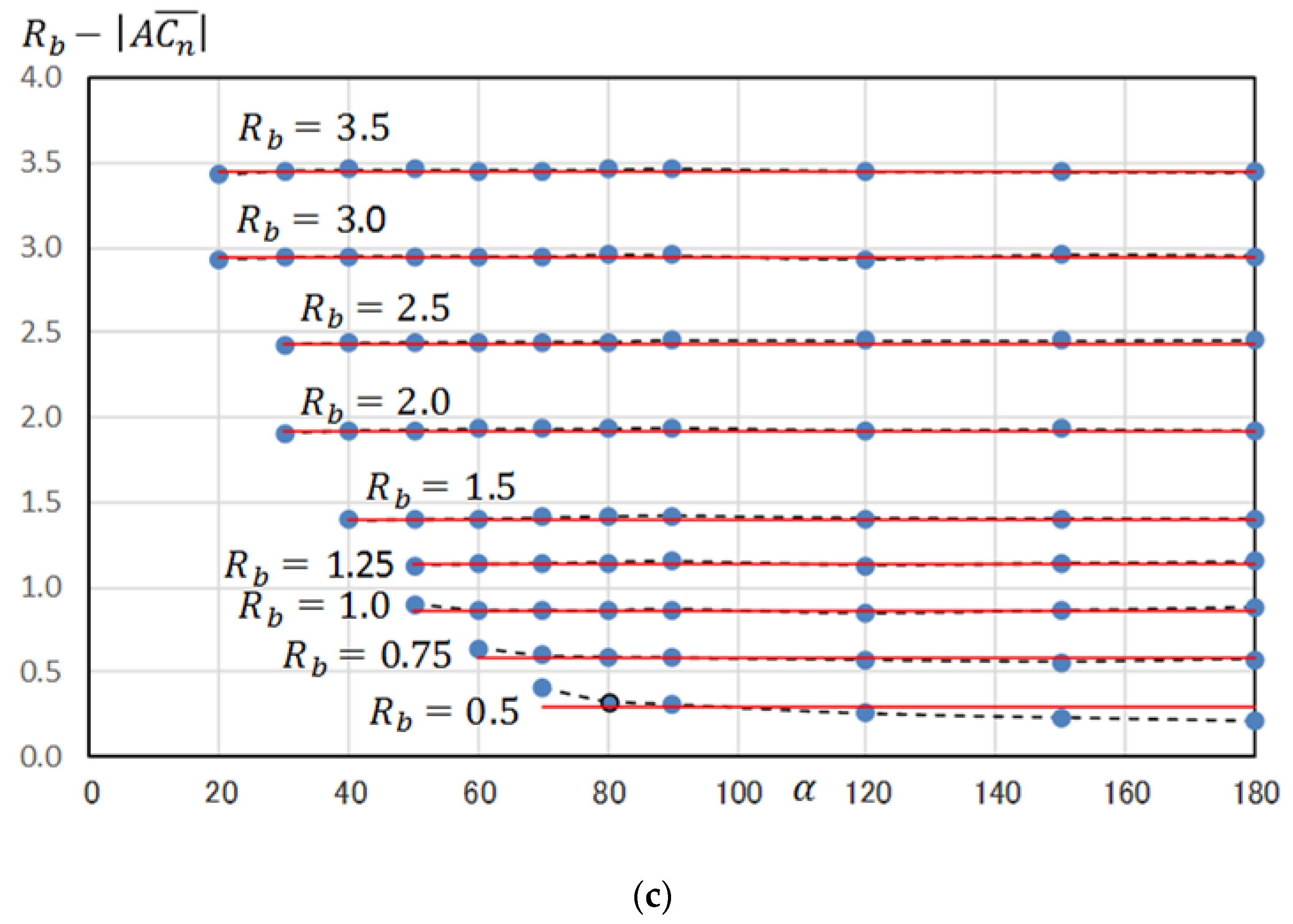
For the trapezoidal dam with vertical entrance face, in the range $R_b\ge 1.00$, the starting point $C$ can be applied as a fixed value that does not depend on $\alpha$ (detailed Table 5, Figure 11c). This is extended to a usual homogeneous dam, and highly accurate discharge and free surface are calculated (Figure 14 and Figure 15). That is, an equivalent trapezoidal dam with vertical entrance face, which is almost equivalent to the discharge and the discharge point of the dam itself, is defined, and the discharge point $y{B}_e$ is estimated from Table 4 based on the similarity law. Finally, interpolation-equivalent KZ flow, KZI$\left(C, B_e\right)$, calculates the discharge and free surface. It has been confirmed that KZI$\left(C, B_e\right)$ almost has an error-within-one-percent estimation in a wide range of $20°\le \theta \le 90°$ and $20°\le \alpha \le 180°$.

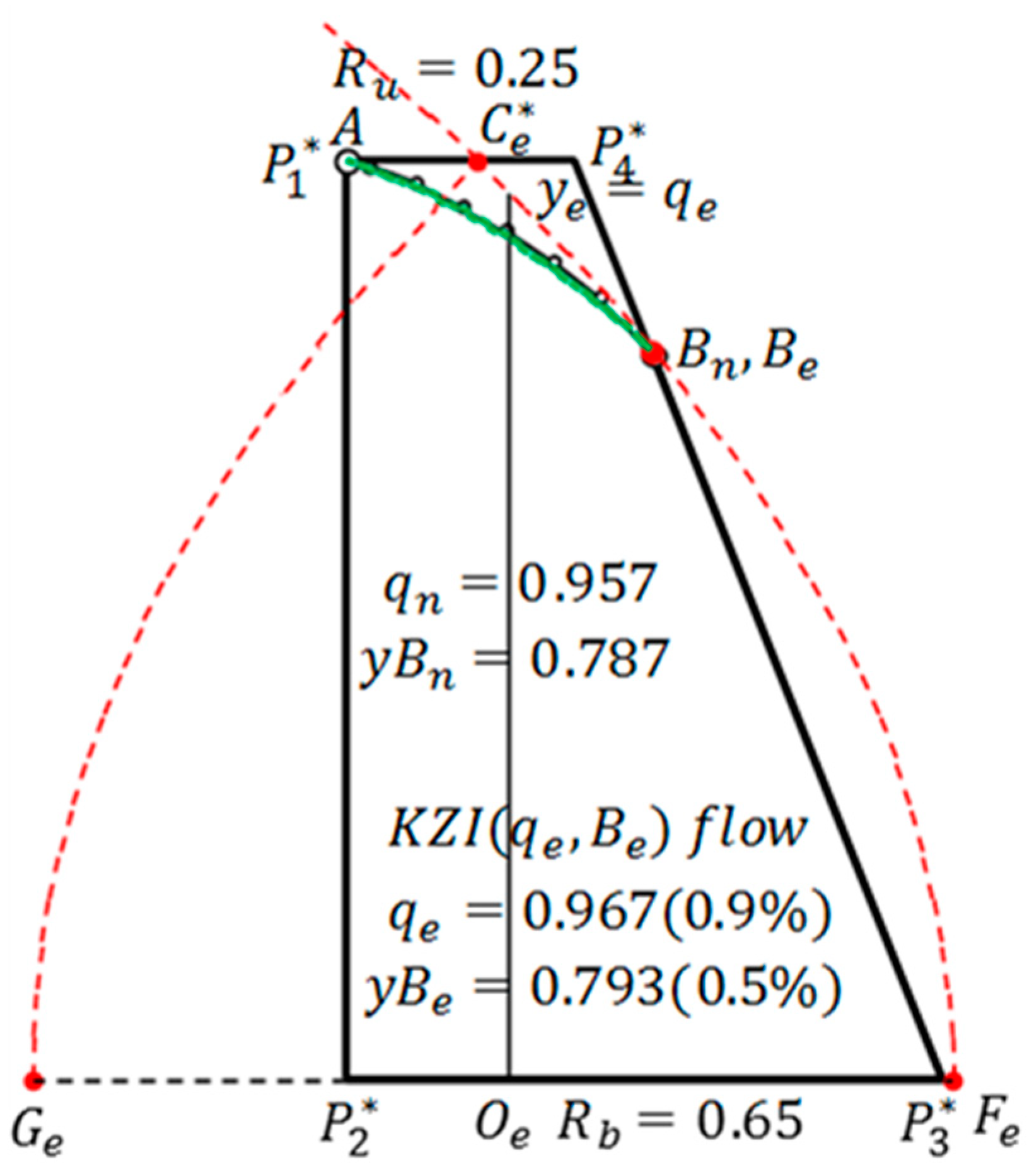
Even in the case of the trapezoidal dam with vertical entrance face, if $R_u\le R_b<1.00$ and as $R_u\to 0$, sufficient accuracy cannot be expected in both KZI($q_e, B_e)$ and KZI($C, B_e)$. In this case, a special method needs to be adopted. In general, the three parameters $q_n,B_n,$ and $C_n$ rapidly change in the process such that the up-side aspect ratio of the trapezoidal dam becomes $R_u\to$ 0; therefore, it is necessary to consider focusing on $R_u$. The following two patterns are investigated:

(i)

For a trapezoidal dam with a vertical entrance face, the equivalent KZ flow is $\mathrm{KZI}\left(q_e, B_e\right)$; the applicable ranges are $R_u\le R_b$, $0.20\le R_u\le 0.50,$ and $0.20\le R_b\le 1.00$.

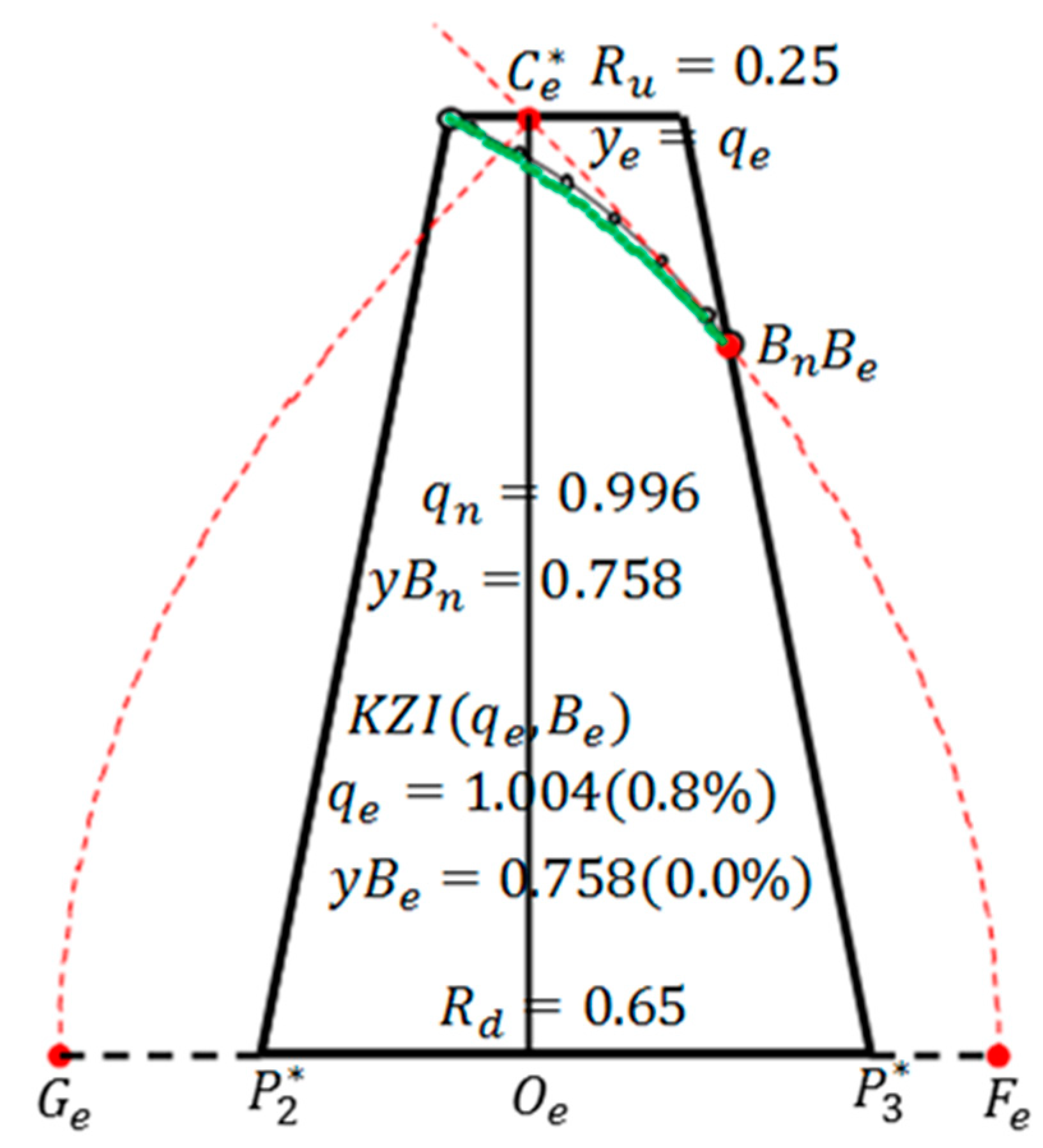
(ii)

For the symmetrical dam center core, the equivalent KZ flow is $\mathrm{KZI}\left(q_e, B_e\right)$; the applicable ranges are$R_u\le R_d$, $0.20\le R_u\le 0.50, \mathrm{and} 0.20\le R_d\le 1.40$.

With the above formulations, the calculation which is practically necessary can be almost covered.

In addition to this, it is necessary to consider separately the cases of inclined core or $\theta >90°$, but $\mathrm{KZn}\left(q_n, B_n\right)$ is also effective in such cases. If the corresponding two-dimensional table is created, it will be possible to perform highly accurate calculation by the same method as that in (1) and (2) above.

Finally, we examined the case of $R_u=R_b$, that is, a rectangular dam. This is already included as a special case in (i) and (ii), but there is a problem to be considered independently. For a rectangular dam, the equivalent KZ flow is ${\mathrm{KZ}}_f\left(q_t, B_f\right)$; the applicable range is $0.2\le R_b\le 1.4$; however, it is finally extended to $0.2\le R_b\to \infty$ according to the concept of “discharge-independent principle”. That is, when the basic aspect ratio, $R_b$, increases to some extent, the discharge phenomenon in the vicinity of the discharge point becomes a phenomenon peculiar to the discharge amount itself, and has no relationship with the shape of the entrance face. This concept is extended to the case of arbitrary $\alpha$. By measuring $yB$, the discharge may be determined by $q=\left(k_c\right)\beta yB$, in which $\beta$ depends on $\alpha$.

The accuracy of the numerical calculation used in this paper was confirmed in the previous paper. The theoretical solution for generally obtaining the discharge and discharge point of a trapezoidal dam with vertical entrance face is in the literature [19]), but it is exceedingly difficult. Lo (1971) [9] numerically evaluated them (discharge and discharge point) and showed this graphically. Based on his graphs, the author confirmed several cases of seepage and it was judged that they were in agreement with the author’s numerical calculation results within some error, but there was a reading error and it could not withstand rigorous evaluation. In relation to this, the graphic display that enables various estimations was valuable in an era when the calculation method was insufficient, and it was also useful for intuitively grasping the whole image. However, now, it is considered that the numeric information that makes a pair with such a graph is essential, because the computer can instantly perform calculation processing using an interpolation method.

In this paper, the validity of the numerical calculation in the correspondence with the theoretical solution is directly confirmed only for the KZ flow and the rectangular dam flow. Regarding the latter, the numerical calculation result and the theoretical solution agree with the discharge, but there may be an error of about 1–2% in the discharge point. From the viewpoint of the goal of this paper, within a few percent of error, it was judged that there is no problem.

Now, let us point out the following. In the calculation of the free surface, there is considerable freedom in setting the initial surface, but many iterative calculations are required until it converges. If the high-accuracy initial surface is set, the calculation is completed by repeating the calculation several times. Theories evolve in stages, from simple to complex, from special to general. As pointed out in Section 5.5, soil materials generally exhibit anisotropy. The general governing equation for anisotropic seepage problems including the case of treating full permeability tensor has already been established (ex. Lei et al. 2015 [21]), and numerical calculation by IFDM-BPIM is possible. Furthermore, a discontinuous line (or plane) of the soil material is formed in the calculation domain. A general numerical calculation system in this case will be built based on the findings confirmed in the previous two papers [4,5] and this paper.