Article

On the Sensitivity of Characteristic Transfer Functions of Multivariable Control Systems

Aerial Robotics Center, National Polytechnic University of Armenia, Yerevan 0009, Armenia
*
Author to whom correspondence should be addressed.
Automation 2026, 7(3), 89; https://doi.org/10.3390/automation7030089
Submission received: 6 April 2026 / Revised: 25 May 2026 / Accepted: 6 June 2026 / Published: 9 June 2026
(This article belongs to the Section Control Theory and Methods)

Abstract

In the paper, a systematic treatment of sensitivity analysis of multivariable cont rol systems within the framework of the characteristic transfer functions (CTFs) method is given. The CTFs method (also called characteristic gain loci method) allows one to associate with an N-dimensional multi-input multi-output (MIMO) system a set of N independent single-input single-output (SISO) characteristic systems and thereby to reduce the analysis and design of a MIMO system to the analysis and design of N SISO systems. The formulas determining the sensitivity functions of the CTFs and the sensitivity vectors of the canonical basis axes to small variations of parameters of general type MIMO systems are derived. The relations between the sensitivity functions of the open-loop and closed-loop MIMO systems are established. Two illustrative examples are considered. The first of them concerns the sensitivity of a two-dimensional non-robust system with a large degree of skewness of the canonical basis axes. In the second example, the sensitivity of the control system of a hexacopter (a multirotor UAV with six rotors) to small degradations in motors efficiency is analyzed.

1. Introduction

Multivariable or multi-input multi-output (MIMO) control systems are ubiquitous in modern industry and technology, including such fields as chemical and power industries, electrical and aerospace engineering, and, especially, robotics, automation, and mechatronics [1,2,3,4]. This article addresses an important issue in multivariable feedback control, which has always attracted the interest of scientists and researchers. In a broader context, the matter concerns the analysis of sensitivity of feedback control systems to small variations of parameters, an issue which is closely related to conventional robustness analysis.
Various aspects of sensitivity analysis of control systems are presented in numerous articles, textbooks, and monographs [5,6,7,8,9,10,11,12,13]. Thus, the bibliography in the monograph “Theory of Sensitivity in Dynamic Systems” by Prof. M. Eslami [7], published in 1994, contained more than 2500 titles on sensitivity theory and related topics. One of the first publications devoted to sensitivity analysis of multivariable feedback systems was the article by J. Cruz and W. Perkins [9], in which some frequency-domain criteria involving the sensitivity matrix were derived.
At present, the theory and methods of multivariable feedback control are mostly inherited from general feedback control [1,2,3,4,14], where optimal, adaptive, robust, and some other methods are predominant [15,16,17,18,19,20,21,22,23,24,25]. For the most part, these methods are based on the state-space representation of control systems, which, being quite effective from the computational perspective and possessing many other substantial features, often lacks the physical clarity inherent in common frequency-domain and root-domain methods of classical feedback control [14]. The point is that many important structural features of multivariable control systems that can be easily seen from the input–output (matrix) description of MIMO systems are often significantly “disguised” in the corresponding state-space equations.
In this respect, in the 1970s, the prominent British theorist A.G. Macfarlane and his colleagues proposed the characteristic transfer functions (CTFs) method (also called characteristic locus or characteristic gain loci method), which was based on the transfer matrix representation of MIMO control systems [26,27,28,29].
Formally, the CTFs method allows one to associate with an N-dimensional (that is having N inputs and N outputs) MIMO system a set of N independent single-input single-output (SISO) characteristic systems, and, as a consequence, to reduce the stability analysis and design of an interconnected MIMO system to stability analysis and design of N SISO systems [1,2,3].
In fact, the ideas of the CTFs method created exceptional opportunities to extend classical feedback control to multivariable systems. However, no effective design procedures for MIMO systems were proposed in [26,27,28,29]. Moreover, the CTFs method was claimed in [24,25] as unreliable and not robust.
In monograph [3], the main classical methods of feedback control were extended to MIMO case based on the CTFs method. The central feature of the methods presented in [3] is that the design of any N-dimensional MIMO system can be reduced to design of a certain SISO system using standard classical methods and techniques.
The concept of characteristic gain loci sensitivity was first introduced by I. Postlethwaite [30]. The sensitivity indices introduced in [30] characterize the sensitivity of the gain loci to small perturbations of the return-ratio matrix of the MIMO system. The sensitivity indices are calculated using the left and right eigenvectors of the return-ratio matrix and provide information about stability with respect to small perturbations of that matrix. The issue of robustness of MIMO systems, where the plant is described using the CTFs method, is addressed in [31]. In that paper, a sophisticated two-stage design procedure to improve system robustness is proposed based on the notion of commutative controller [29]. At the first stage, a dynamic pre-compensator is designed which transforms, at least at some predefined frequencies, the plant transfer matrix into a normal matrix. Then, at the second stage, a commutative controller is designed for the pre-compensated (normalized) plant. If the design is correct, then the corresponding CTFs of the pre-compensated plant and the commutative controller are simply multiplied together. However, in general, it is impossible to find a realizable matrix compensator that transforms the transfer matrix of the plant into a normal matrix. For that reason, there are no effective design procedures based on the notion of commutative controllers.
A broadened discussion of modern sensitivity-analysis methodology can be found, for example, in [32,33,34].
At the same time, many important aspects of sensitivity of MIMO systems, such as the sensitivity of canonical basis axes and relation between the sensitivities of the CTFs of open-loop and closed-loop systems, have not been discussed in [30,31] or in any other publications.
In this paper, the issue of sensitivity of general type MIMO systems to small variations of parameters is systematically addressed within the framework of the CTFs method.
The paper is organized as follows. A short presentation of the main ideas of the CTFs method is given in Section 2. Section 3 is the central and is devoted to derivation of formulas determining the sensitivity of the CTFs and the canonical basis axes to small variations (perturbations) of parameters. Section 4 presents two illustrative examples of applying the results of the previous section to specific MIMO control systems. The first of them describes the notorious two-dimensional system that was used in [24,25] as an example, illustrating that the CTFs method is not robust. In that section, a detailed explanation is given as to why the conclusions made in [24,25] are erroneous. The second example concerns the sensitivity analysis of the hexacopter’s control system to small degradations of motors efficiency.

2. Canonical Representation of MIMO Control Systems

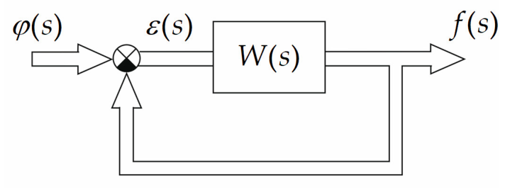
Consider an N-dimensional MIMO feedback control system in Figure 1. Here, φ ( s ) ,   f ( s ) ,   ε ( s ) denote the Laplace transforms of the N-dimensional input, output, and error vector signals φ ( t ) ,   f ( t ) ,   ε ( t ) , respectively (we shall regard them as elements of some N-dimensional complex space N ); W ( s ) = { w k r ( s ) } is a square transfer function matrix of the open-loop system of order N × N with entries w k r ( s ) ( k , r = 1 , 2 , , N ) which are scalar proper rational functions in complex variable s [3].
The output f ( s ) and error ε ( s ) vectors, where
ε ( s ) = φ ( s )     f ( s ) ,
are related to the input vector φ ( s ) by the following operator equations:
f ( s ) = T ( s ) φ ( s )   ,                       ε ( s ) = S ( s ) φ ( s )
where
T ( s ) = I + W ( s ) 1 W ( s ) ,       S ( s ) = I + W ( s ) 1
are the transfer function matrices of the closed-loop MIMO system with respect to output and error signals, and I is the unit matrix. The transfer matrices S ( s ) and T ( s ) are usually called the sensitivity function matrix and complementary sensitivity function matrix [3].
Based on the method of characteristic transfer functions (CTF), the transfer matrix of the open-loop MIMO system W ( s ) can be represented, using dyadic notation and similarity transformation, in the following canonical forms [3]:
W ( s ) = i = 1 N c i ( s )   >   q i ( s )   <   c i + ( s ) = C ( s ) d i a g { q i ( s ) } C 1 ( s ) ,
where the complex scalar function q i ( s ) ( i = 1 , 2 , , N ) (“eigenvalues” of W ( s ) ) are called the CTFs of the open-loop system (further, for simplicity, all q i ( s ) are assumed distinct); c i ( s ) are linearly-independent normalized eigenvectors of W ( s ) which constitute the canonical basis of the open-loop MIMO system; c 1 + ( s ) are vectors dual to c i ( s ) (vectors of the dual basis), and the modal matrix C ( s ) is composed of vector-columns c i ( s ) .
Substitution the canonical representations of W ( s ) (4) into the complementary sensitivity function matrix T ( s ) and the sensitivity function matrix S ( s ) (3) yields
T ( s ) = i = 1 N c i ( s )   >   q i ( s ) 1 + q i ( s )   <   c i + ( s ) = C ( s ) d i a g q i ( s ) 1 + q i ( s ) C 1 ( s )
S ( s ) = i = 1 N c i ( s )   >   1 1 + q i ( s )   <   c i + ( s ) = C ( s ) d i a g 1 1 + q i ( s ) C 1 ( s )
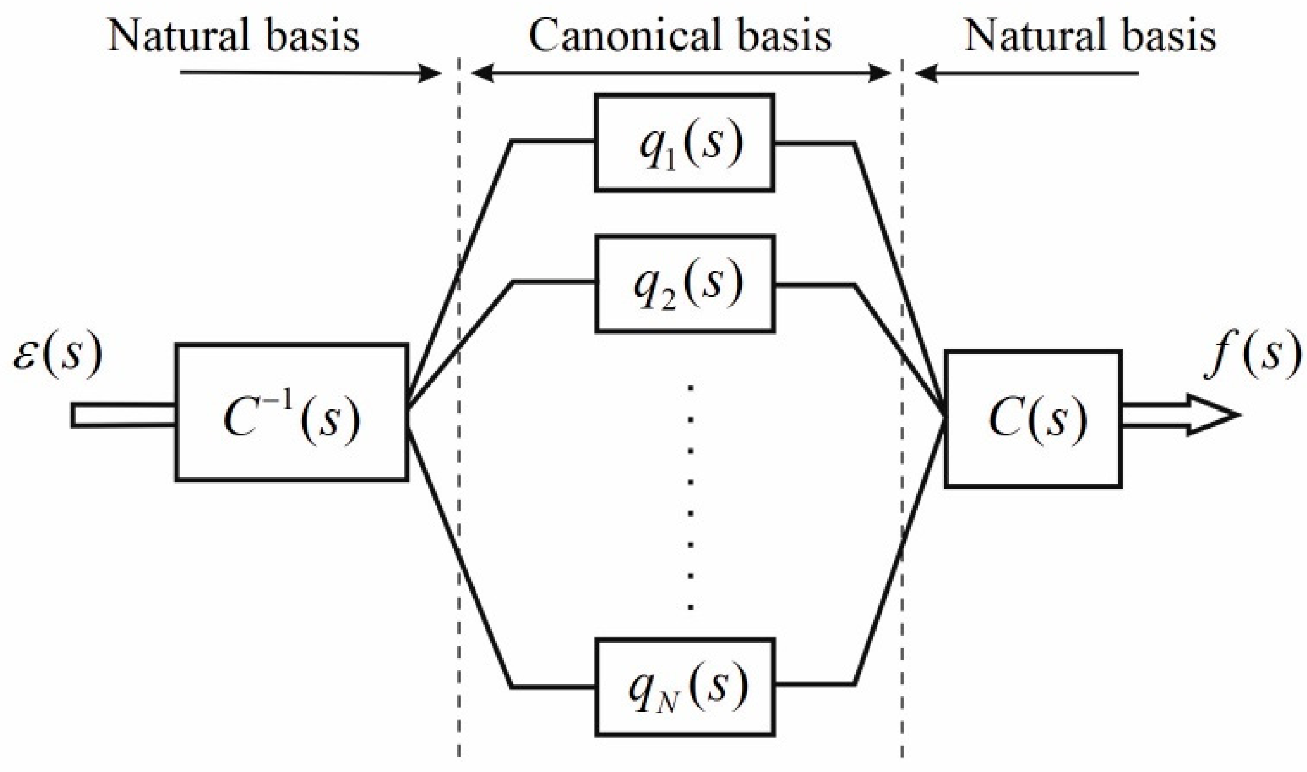
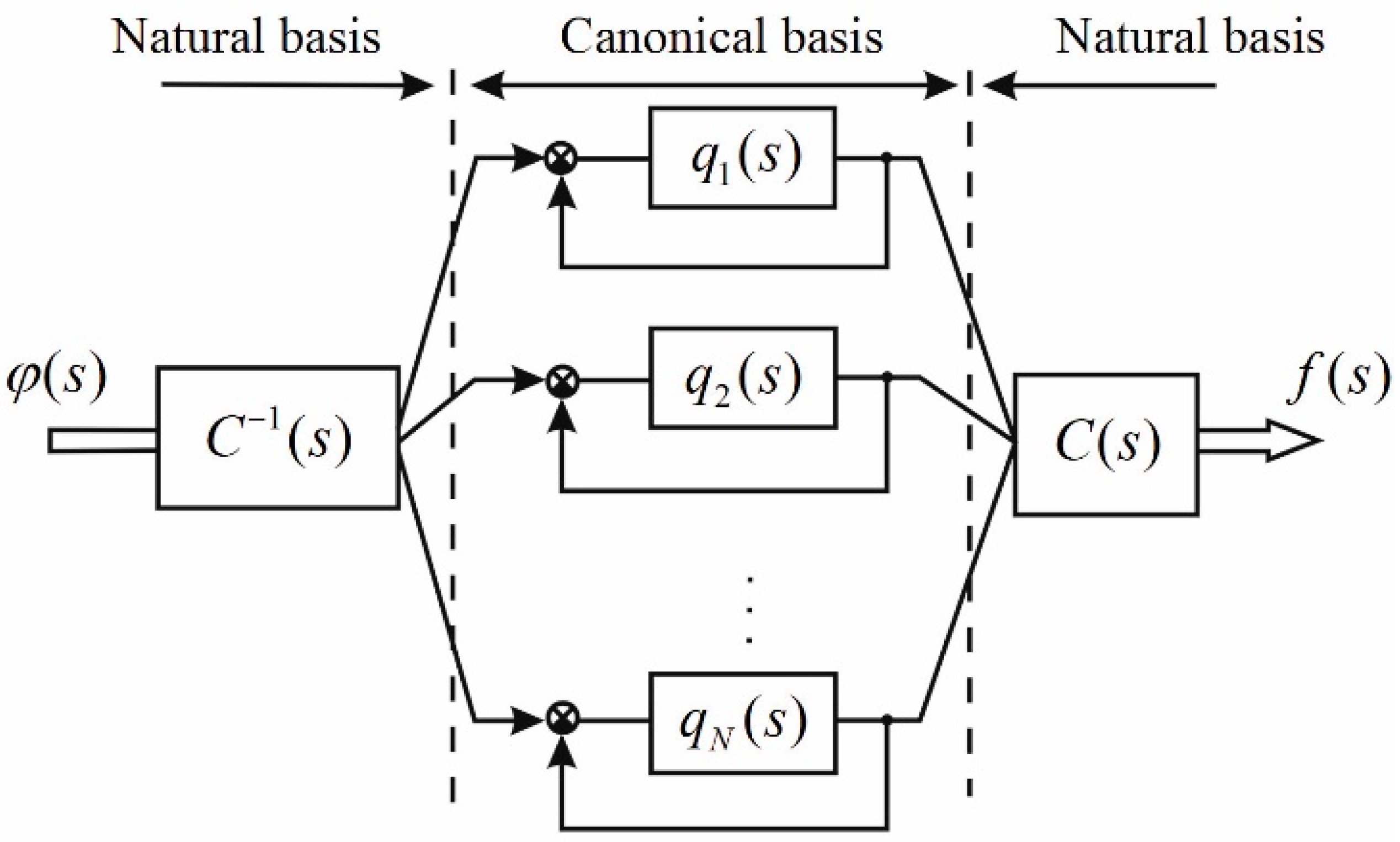
Examination of (4)–(6) shows that the canonical basis of the closed-loop MIMO system coincides with the canonical basis of the open-loop system [3]. Moreover, the CTFs of the closed-loop MIMO system with respect to the output and error are related to q i ( s ) by the very same relationships as common transfer functions of open-loop and closed-loop SISO feedback systems. Geometrically, all this is illustrated in Figure 2 and Figure 3.
The stability of the multivariable system in Figure 1 is determined by the roots of the characteristic equation [1,2,3].
det [ I + W ( s ) ] = i = 1 N [ 1 + q i ( s ) ] = 0
As can be seen from (7), the multivariable system in Figure 1 is stable if all N SISO characteristic systems are stable. Note that the stability of characteristic systems can be analyzed using conventional methods of classical feedback control, in particular, the Nyquist criterion [1,3,14].
It should also be noted that the generally accepted assumption of no repeated CTFs is well justified and not restrictive in practical calculations [3].
Rigorously speaking, the CTFs of general-type transfer matrices belong to the class of multi-valued algebraic functions and constitute one mathematical entity. The branches of the characteristic gain loci are situated on different sheets of a Riemann surface. Transition from one sheet to another is accomplished through the “cuts” connecting the point at infinity with the branch points of the algebraic function, at which two or more CTFs are equal.
When solving practical engineering tasks, the behavior of CTFs in the neighborhood of branch points is neglected, and for any fixed complex or real value s = c o n s t , not coinciding with the branch points, the transfer matrix W ( s ) may be viewed as a usual numerical matrix with complex entries. Then, the problem of finding the CTFs for that value of s is simply reduced to computing the eigenvalues of the numerical matrix W ( s ) .
On the other hand, the transfer matrices of MIMO systems are composed of scalar transfer functions which are linear approximations of some dynamic SISO objects. The parameters of these transfer functions are always specified with a certain accuracy, and it is always possible to change the parameters of any individual SISO transfer function, within the given specification accuracy, in a way that excludes the presence of multiple CTFs for any value s = c o n s t .

3. Sensitivity of Characteristic Transfer Functions and Canonical Basis Axes

In this section, we discuss, from the standpoint of the CTFs method, the influence of small perturbations (variations) of parameters on the structural and geometrical features of linear MIMO systems. The main attention is paid to the sensitivity functions of SISO characteristic systems and canonical basis axes in the case of small variations of the MIMO system parameters.
Consider the linear MIMO system in Figure 1 and assume that the open-loop transfer matrix W ( s ) depends continuously on m varying parameters α r   ( r = 1 ,   2 ,     ,   m ) , forming the vector α . Furthermore, to emphasize the dependence of W ( s ) on α , we shall write W ( s , α ) . Denote by α ο the vector of nominal values of α , and by Δ α , the vector of variations, i.e., assume α = α ο + Δ α . Let the CTFs and canonical basis of the MIMO system with the nominal values α ο be known. A question arises: How are the CTFs and canonical basis axes changed in the case of small variations of the parameters α , i.e., for ( Δ α r ) 2     0 ? We solve this task as a first approximation, based on the perturbation theory of linear operators in finite-dimensional Hilbert spaces [35,36].
Because of parameters perturbations, let the transfer matrix W ( s , α ο ) be expressed as
W ( s , α ) = W ( s , α ο ) + Δ W ( s , α )
where Δ W ( s , α ) is the variation of W ( s , α ο ) caused by the perturbations Δ α . As we assume continuous dependence of W ( s , α ) on α r , the variation Δ W ( s , α ) in (8) can be represented, for small Δ α r , with the help of the Taylor series:
Δ W ( s , α ) = r = 1 m U r W ( s ) Δ α r   +
where
U r W ( s ) = δ W ( s , α ) δ α r α = α ο                 r = 1 ,   2 ,     ,   m
are the first-order sensitivity matrices of the transfer matrix W ( s , α ) with respect to variations Δ α r , evaluated for the nominal vector α = α ο . The dots in (9), and in what follows, mean that the terms of the higher order of smallness, as compared with Δ α r , are omitted.
As W ( s , α ) is assumed differentiable with respect to α r , the following expansions for the CTFs q i ( s , α ) and the canonical basis axes c i ( s , α ) are valid:
q i ( s , α ) = q i ( s , α ο ) + r = 1 m S i r q ( s ) Δ α r +
and
c i ( s , α ) = c i ( s , α ο ) + r = 1 m ϒ i r q Δ α r + , i = 1 ,   2 ,     ,   N
where
S i r q ( s ) = δ q i ( s , α ) δ α r α = α ο ,                         ϒ i r q ( s ) = δ c i ( s , α ) δ α r α = α ο                                                       r = 1 ,   2 ,     , m
are the unknown first-order sensitivity functions of q i ( s , α ) and sensitivity vectors of c i ( s , α ) .
Since (11) and (12) are the eigenvalues and eigenvectors of the varied matrix W ( s , α ) (8), and allowing for (9), we can write
W ( s , α ο ) + r = 1 m U r W ( s ) Δ α r   +   c i ( s , α ο ) + r = 1 m ϒ i r q Δ α r + = q i ( s , α ο ) + r = 1 m S i r q ( s ) Δ α r + c i ( s , α ο ) + r = 1 m ϒ i r q Δ α r + r = 1 ,   2 ,     ,   m
Carrying out the multiplication and comparing the first-order terms with respect to the corresponding perturbations Δ α r on both sides of (14), we obtain the following system of m N equations:
U r W ( s ) c i ( s , α ο ) + W ( s , α ο ) ϒ i r q ( s ) = q i ( s , α ο ) ϒ i r q ( s ) + S i r q ( s ) c i ( s , α ο )                                                               i = 1 ,   2 ,     ,   N ;         r = 1 ,   2 ,     ,   m
Multiply, in the form of a scalar product, both sides of (15) by the vector c i + ( s , α ο ) , which is dual to the eigenvector c i ( s , α ο ) of the initial (unperturbed) MIMO system. Recalling that the first vector in the scalar product should be taken as the complex conjugate, we obtain
< U r W ( s ) c i ( s , α ο ) , c i + ( s , α ο ) > + < W ( s , α ο ) ϒ i r q ( s ) , c i + ( s , α ο ) >   =                     q ˜ i ( s , α ο ) < ϒ i r q ( s ) , c i + ( s , α ο ) > + S ˜ i r q ( s )                                       i = 1 ,   2 ,     ,   N ;             r = 1 ,   2 ,     ,   m
Note that if the matrix W ( s , α ο ) has the canonical representation
W ( s , α ο ) = C ( s , α ο ) d i a g { q i ( s , α ο ) } C 1 ( s , α ο )
then the conjugate matrix W * ( s , α ο ) is
W * ( s , α ο ) = ( C 1 ( s , α ο ) ) * d i a g { q ˜ i ( s , α ο ) } C * ( s , α ο ) .
From here, it is clear that the eigenvector c i + ( s , α ο ) , which is dual to the eigenvector c i ( s , α ο ) of W ( s , α ο ) , corresponds to the CTF q ˜ i ( s , α ο ) of W * ( s , α ο ) . Therefore,
< W ( s , α ο ) ϒ i r q ( s ) , c i + ( s , α ο ) > = < ϒ i r q ( s ) , W * ( s , α ο ) c i + ( s , α ο ) >                                     =   q ˜ i ( s , α ο ) < ϒ i r q ( s ) , c i + ( s , α ο ) >
Substituting (19) into (16) and conjugating both sides in (16) yields the final expression for the sensitivity function S i r q ( s ) :
S i r q ( s ) = < c i + ( s , α ο ) , U r W c i ( s , α ο ) > i = 1 ,   2 ,     ,   N ;               r = 1 ,   2 ,     ,   m .
It is important to note that, for any fixed r , the right sides in (20) represent (for i = 1 ,   2 ,     ,   N ) the diagonal elements of the matrix U r W ( s ) (10), where the latter is evaluated in the basis composed of the vectors c i ( s , α ο ) . Hence, the open-loop MIMO system sensitivity functions S i r q ( s ) with respect to small perturbations of the r th parameter α r are equal to the diagonal elements of the sensitivity matrix U r W ( s ) evaluated in the canonical basis of the unperturbed MIMO system. Multiplying both sides in (16) by Δ α r , we come to the conclusion that a similar relationship takes place, as a first approximation, between the finite variations Δ q i r = S i r W Δ α r and the diagonal elements of the matrix of finite variations Δ W r ( s ) = U r W ( s ) Δ α r .
Proceed now to the sensitivity vectors ϒ i r q ( s ) (13) of the open-loop MIMO system’s canonical basis axes. Toward this end, multiply both sides of (15) by the dual vectors c k + ( s , α ο )   ( k = 1 ,   2 ,     ,   N ;       k     i ) . After some simple transformations, this yields
< c k + ( s , α ο ) , ϒ i r q ( s ) > = n k i r ( s ) q i ( s , α ο )     q k ( s , α ο ) k = 1 ,   2 ,     ,   N ;       k     i ,             r = 1 ,   2 ,     ,   m ,
where
n k i r ( s ) = < c k + ( s , α ο ) , U r W ( s ) c i ( s , α ο ) >
are the elements of the i th column (except for n i i r ( s ) ) of the matrix U r W ( s ) (10), represented in the canonical basis of the unperturbed MIMO system. Notice that the scalar products on the left side of (21) are the coordinates of the vector ϒ i r q ( s ) along the k th axis c k ( s , α ο ) of the initial canonical basis. It is easy to show, using the normalizing condition for the varied eigenvector c i ( s , α ο ) (12) [35], that the coordinate of ϒ i r q ( s ) along the i th axis c i ( s , α ο ) is equal to zero. Therefore, we can write
ϒ i r q ( s ) = k = 1 k     i N n k i r ( s ) q i ( s , α ο )     q k ( s , α ο ) c k ( s , α ο ) ,     i = 1 ,   2 ,     ,   N ;           r = 1 ,   2 ,     ,   m      
Thus, Expressions (20)–(22) determine the sensitivity functions S i r q ( s ) of the CTFs q i ( s , α ) of the open-loop MIMO system and the sensitivity vectors ϒ i r q ( s ) of the canonical basis axes c i ( s , α ) with respect to small perturbations of the parameters α r . These expressions show that for evaluating S i r q ( s ) and ϒ i r q ( s ) it is enough to find the representation
N r ( s ) = C 1 ( s , α ο ) U r W ( s ) C ( s , α ο )   ,                             r = 1 ,   2 ,     ,   m
of the matrices U r W ( s ) (10) in the canonical basis of the unperturbed MIMO system. The diagonal elements n i i r ( s ) of the matrix N r ( s ) (23) are equal to S i r q ( s ) , and the non-diagonal elements n i k r ( s ) , after dividing by the differences [ q i ( s , α ο )     q k ( s , α ο ) ] , give the coordinates of ϒ i r q ( s ) in the aforementioned basis.
Consider now the sensitivity of the closed-loop MIMO system, restricting ourselves, for brevity, to the sensitivity transfer matrix S ( s ) (3). Assume that because of the parameter’s perturbations Δ α , the initial transfer matrix S ( s , α ο ) becomes
S ( s , α ) = S ( s , α ο ) + Δ S ( s , α ) ,
where Δ S ( s , α ) is the variation of S ( s , α ο ) caused by the perturbations Δ α . Let us find the expression for S ( s , α ) , assuming that the corresponding variation Δ W ( s , α ) of the open-loop MIMO system is known. In that case, the matrix S ( s , α ) (24) can be represented in the form
S ( s , α ) = [ I + W ( s , α ο ) + Δ W ( s , α ) ] 1
From (3) and (12), it is easy to see that the variation Δ W ( s , α ) is equal to the difference of the inverse transfer matrices S 1 ( s , α ) and S 1 ( s , α ο ) , i.e.,
S 1 ( s , α )     S 1 ( s , α ο ) = Δ W ( s , α ) .
Multiplying this relation from the left by S ( s , α ο ) and from the right by S ( s , α ) yields
S ( s , α ο )     S ( s , α ) = Δ S ( s , α ) = S ( s , α ο ) Δ W ( s , α ) S ( s , α )
from which, taking into account (24), and after simple algebraic transformations, we obtain the following expression for the variation Δ S ( s , α ) of the transfer matrix S ( s , α ο ) caused by the variation Δ W ( s , α ) :
Δ S ( s , α ) = [ I + S ( s , α ο ) Δ W ( s , α ) ] 1 S ( s , α ο ) Δ W ( s , α ) S ( s , α ο )
In principle, this expression is valid for any, not necessarily small, variations Δ W ( s , α ) . Recalling that the task above was solved as a first approximation, preserving only the terms linear with respect to Δ α r , let us determine this approximation for Δ S ( s , α ) . To this end, expand the inverse matrix on the right side of (27) into the infinite Neumann series [36]:
[ I + S ( s , α ο ) Δ W ( s , α ) ] 1 = i = 0 [ S ( s , α ο ) Δ W ( s , α ) ] i
This series converges for | | S ( s , α ο ) Δ W ( s , α ) | |   <   1 , which always takes place in practice for small Δ α r . Substituting (28) in (27), and neglecting the terms of the higher order of smallness, gives a first approximation for the variation Δ S ( s , α )
Δ S ( s , α ) = S ( s , α ο ) Δ W ( s , α ) S ( s , α ο ) .
Owing to the continuous dependence of the transfer matrix S ( s , α ) on parameters α r , the variation Δ S ( s , α ) can be written in the form
Δ S ( s , α ) = r = 1 m U r S ( s ) Δ α r + ,
where
U r S ( s ) = δ S ( s , α ) δ α r α = α ο             r = 1 ,   2 ,     ,   m
are the first-order sensitivity matrices of the transfer matrix S ( s , α ) with respect to the variations of the r th parameter α r . Then, based on (29), (30), and (9), we find the following formulae establishing relationships between the sensitivity matrices (10) and (31) of the open-loop and closed-loop MIMO system transfer matrices:
U r S ( s ) = S ( s , α ο ) U r W ( s ) S ( s , α ο )                             r = 1 ,   2 ,     ,   m .
The CTFs S i ( s ) of the closed-loop MIMO system have the following form:
S i ( s , α ) = 1 1 + q i ( s , α )           i = 1 ,   2 ,     ,   N .
These functions are expanded into the Taylor series:
S i ( s , α ) = S i ( s , α ο ) + r = 1 m S i r S ( s ) Δ α r + ,                                     i = 1 ,   2 ,     ,   N ,
where
S i r S ( s ) = δ S i ( s , α ) δ α r α = α ο             r = 1 ,   2 ,     ,   m
are the first-order sensitivity functions of the CTFs S i ( s , α ) with respect to the variations of the r th parameter α r .
Since the canonical bases of the open-loop and closed-loop MIMO system coincide, Expansion (12) is also valid for the axes c i ( s , α ) of the closed-loop system, where, instead of ϒ i r q ( s ) , the designations ϒ i r S ( s ) should be introduced. Proceeding in the same manner as in the analysis of the open-loop MIMO system, it is easy to show that, for evaluating S i r S ( s ) and ϒ i r S ( s ) , it is necessary to find the representation of the matrices U r S ( s ) (31) in the canonical basis of the unperturbed MIMO system. That representation has the form
M r ( s ) = C 1 ( s , α ο ) U r S ( s ) C ( s , α ο )                           r = 1 ,   2 ,     ,   m
The diagonal elements m i i r ( s ) of the matrix M r ( s ) are equal to the sensitivity functions S i r S ( s ) (34), and the non-diagonal elements m k i r ( s ) , divided by the differences [ S i ( s , α ο )     S k ( s , α ο ) ]   ( k = 1 ,   2 ,     , N ,   k     i ) , yield the coordinates of the sensitivity vectors ϒ i r S ( s ) of the i th canonical axis of the closed-loop MIMO system.
Expressions (32) and (35) enable us to determine the relationship between sensitivity functions of the open-loop and closed-loop MIMO system, i.e., to determine the effect caused on the MIMO system sensitivity by the introduction of feedback. Substituting (32) into (35), using the canonical representation of the transfer matrix S ( s , α ο ) (47) and accounting for (23), gives
M r ( s ) = d i a g 1 1 + q i ( s , α ο ) N r ( s ) d i a g 1 1 + q i ( s , α ο )                                                         r = 1 ,   2 ,     ,   m
from which, finding the diagonal elements on the right side, we obtain
S i r S ( s ) = 1 [ 1 + q i ( s , α ο ) ] 2 S i r q ( s )   i = 1 ,   2 ,     , N ;       r = 1 ,   2 ,     ,   m .
Expressions (37) relate the sensitivity functions of the closed-loop and open-loop SISO characteristic systems and are completely analogous to those well known in the classical control theory [5,14]. If we let s = j ω , then from (37) it is clear that, for those frequencies ω for which | q i ( j ω , α ο ) |   > >   1 (usually it is the low-frequency region), the introduction of feedback decreases the sensitivity of the CTFs to parameters variations. In the high-frequency region, where | q i ( j ω , α ο ) |     0 , the sensitivity of the closed- loop and open-loop CTFs is approximately the same. Finally, in the region of the resonance frequencies, where | S i ( j ω , α ο ) |   >   1 , the feedback deteriorates the sensitivity of the CTFs.
The non-diagonal elements m k i r ( s ) of the matrix M r ( s ) (36) have the form
m k i r ( s ) = n i k r ( s ) [ 1 + q i ( s , α ο ) ] [ 1 + q k ( s , α ο ) ]                     k , i = 1 ,   2 ,     ,   N ;       ( k     i ) .
Dividing both sides of (38) by the differences [ S i ( s , α ο )     S k ( s , α ο ) ] , we obtain the following equalities:
m k i r ( s ) S i ( s , α ο )     S k ( s , α ο ) = n k i r ( s ) q i ( s , α ο )     q k ( s , α ο )                     k , i = 1 ,   2 ,     ,   N ;       ( k     i ) .
But, according to the above statement, the left-hand terms in (39) are equal (for some i ) to the coordinates of the sensitivity vectors ϒ i r S ( s ) of the i th canonical axis of the closed-loop MIMO system, and the right-hand terms are equal to the coordinates of the sensitivity vectors ϒ i r q ( s ) of the corresponding (in fact, the same) axis of the open-loop system. Additionally, all these coordinates are determined with respect to the same canonical basis of the unperturbed MIMO system.
Consequently, the vectors ϒ i r S ( s ) and ϒ i r q ( s ) are equal to each other, i.e., the introduction of feedback does not affect the sensitivity of the MIMO system canonical basis to small variations of parameters.

4. Examples

4.1. Two-Dimensional Non-Robust System

Below, we consider the celebrated example from [24,25], owing to which an erroneous conclusion about inefficiency and lack of robustness of the CTFs method has become quite common in the technical literature.
Given the two-dimensional open-loop system with the following transfer function matrix:
W ( s ) = 1 ( s + 1 ) ( s + 2 ) 47 s + 2 56 s 42 s 50 s + 2 ,
which can be represented in the form
W ( s ) =   7 8 6 7 1 s + 1 0 0 2 s + 2 7 8 6 7 ,
Expression (41) means that, for this system, the CTFs q 1 ( s ) and q 2 ( s ) have the form of first order transfer functions:
q 1 ( s ) = 1 s + 1 ,                   q 2 ( s ) = 2 s + 2 ,
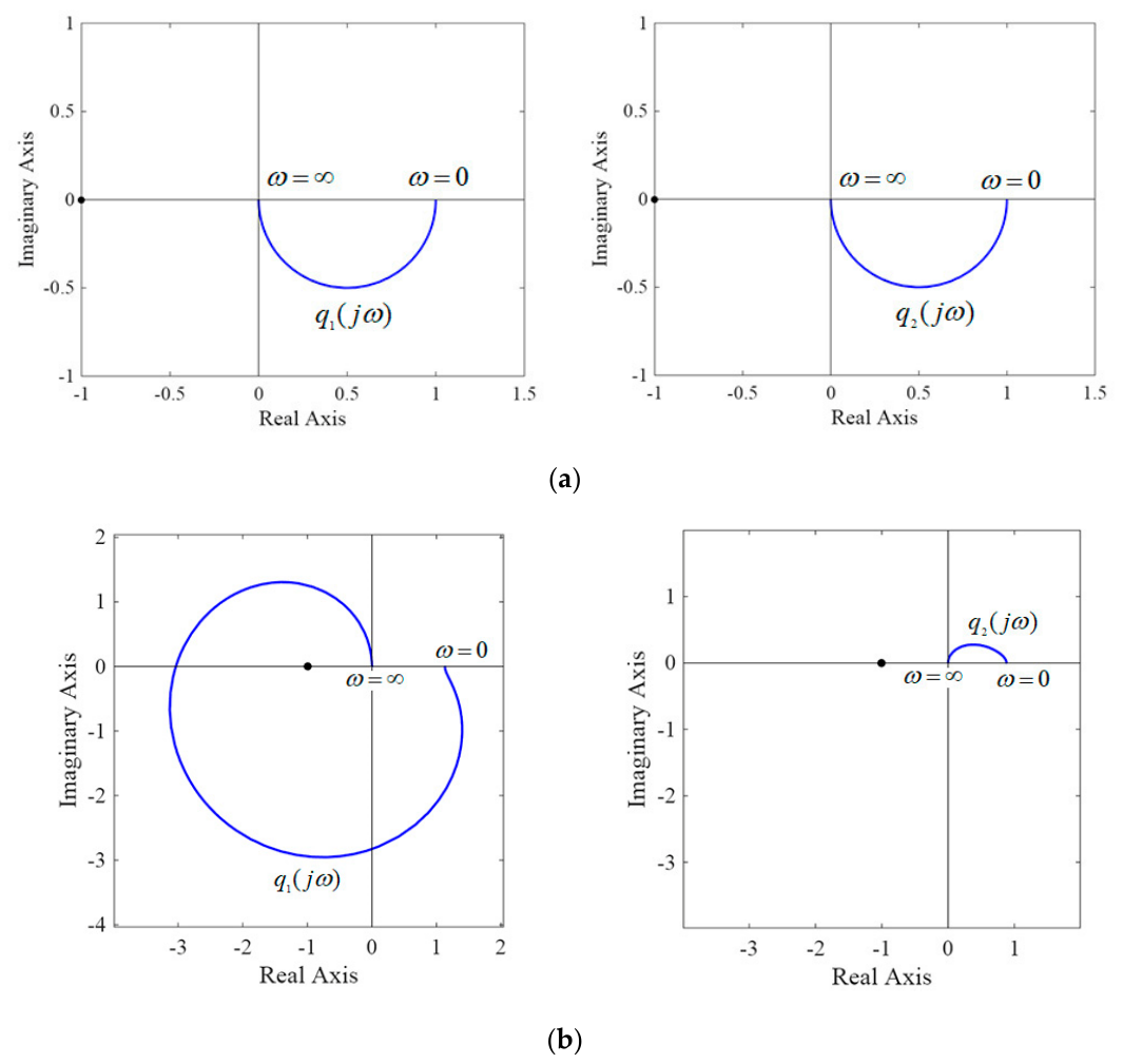
which imply an infinite gain margin and phase margin equal to 180 . The gain loci q 1 ( j ω ) and q 2 ( j ω ) of the system are shown in Figure 4a and confirm that conclusion.
However, as shown in [24], introducing into the system a diagonal regulator
K = 1.13 0 0 0.88 ,
i.e., increasing the gain of the first channel by 0.13 and decreasing the of the second channel by 0.12 , makes the closed-loop system unstable.
At first glance, this indisputable evidence that the stability margins calculated with the help of the CTFs may lead to a wrong conclusion, in fact, demands more careful treatment. As is shown in [3], the discussed MIMO system indeed remains stable for arbitrary large but identical gains in the separate channels, since in that case the canonical basis of the system is unchanged. However, if the matrices W ( s ) (41) and K (43) are multiplied, then the resulting modal decomposition of the system changes drastically. The characteristic gain loci q 1 ( j ω ) and q 2 ( j ω ) of the system with the regulator K (43) are shown in Figure 4b, from which it is clear that the MIMO system is unstable, and its new CTFs are very far from those in Figure 4a.
Let us now discuss the sensitivity of that system with respect to additive perturbations of gains of the diagonal controller. Let the nominal values of the gains be unity and designate their small perturbations by Δ K 1 and Δ K 2 . Then, the open-loop system can be represented as
W ( s ) = 64.5368 73.7564 63.7809 74.4111 C 1 1 s + 1 0 0 2 s + 2 0.7593 0.7526 0.6508 0.6885 C 1 + Δ K 1 0 0 1 + Δ K 2
where, unlike in (41), the columns of the modal matrix C are normalized. It is easy to compute that the matrices N 1 ( s ) and N 2 ( s ) (23), in this case, are
N 1 ( s ) =     49 s + 1     56 s + 1 84 s + 2 96 s + 2 ,                       N 2 ( s ) = 48 s + 1 56 s + 1   84 s + 2     98 s + 2
Since the diagonal elements of N 1 ( s ) , N 2 ( s ) (45) are equal to the sensitivity functions S i 1 q ( s ) and S i 2 q ( s )   ( i = 1 ,   2 ) of the open-loop CTFs with respect to Δ K 1 and Δ K 2 , the CTFs of the varied open-loop system can be represented, as a first approximation, based on (11)–(13), in the form
q 1 ( s ) = 1 s + 1 + 49 s + 1 S 11 q ( s ) Δ K 1     48 s + 1 S 21 q ( s ) Δ K 2 ,           q 2 ( s ) = 2 s + 2     96 s + 2 S 12 q ( s ) Δ K 1 + 98 s + 2 S 22 q ( s ) Δ K 2
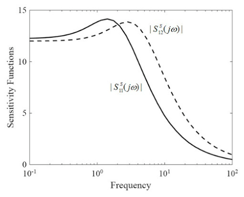
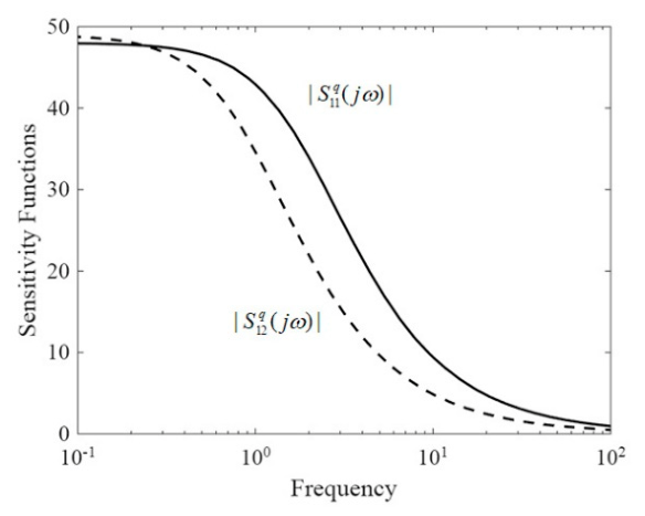
The magnitude plots | S 11 q ( j ω ) | and | S 12 q ( j ω ) | of the first open-loop characteristic system are shown in Figure 5. Similar plots for the second characteristic system practically coincide with those in Figure 5.
Inspection of these plots shows that the CTFs of the open-loop system are very sensitive, in the low-frequency region, to the variations Δ K 1 and Δ K 2 . Thus, at the zero frequency ω = 0 , the sensitivity functions S i 1 q ( s ) and S i 2 q ( s )   ( i = 1 ,   2 ) are equal to
S 11 q ( j 0 ) = 49 ,         S 21 q ( j 0 ) = 48 ,         S 12 q ( j 0 ) = 48 ,         S 22 q ( j 0 ) = 49 .
Furthermore, inspection of (46) allows us to draw interesting conclusions concerning the character of influence of variations Δ K 1 and Δ K 2 . The most dangerous are variations of different signs. Thus, if we assume that Δ K 1 and Δ K 2 are equal by their absolute values and have opposite signs, i.e., Δ K 2 = Δ K 1 (assuming for definiteness Δ K 1   >   0 ), then instead of (46) we obtain
q 1 ( s ) = 1 s + 1 + 97 s + 1 | Δ K 1 |   ,                   q 2 ( s ) = 2 s + 2     194 s + 2 | Δ K 2 |
where the additive variations Δ q i ( s ) of the CTFs have opposite signs. At the same time, in case of equal perturbations Δ K 1 = Δ K 2 = Δ K , we have
q 1 ( s ) = 1 + Δ K s + 1     ,                   q 2 ( s ) = 2 ( 1 + Δ K ) s + 2   ,
i.e., the variations of the CTFs are proportional to Δ K .
Let us proceed now to the sensitivity of the canonical basis axes. For the normalized canonical basis axes of the varied system, based on (13), (23), (44), and (45), and carrying out some simple transformations, we have
c 1 ( s ) = 0.7593 0.6508 + 42 ( s + 1 ) s   0.7593 0.6508 ϒ 11 q ( s ) Δ K 1     42 ( s + 1 ) s   0.7593 0.6508 ϒ 21 q ( s ) Δ K 2
c 2 ( s ) = 0.7526 0.6885 + 28 ( s + 2 ) s   0.7526 0.6885 ϒ 21 q ( s ) Δ K 1     28 ( s + 2 ) s   0.7526 0.6885 ϒ 22 q ( s ) Δ K 2
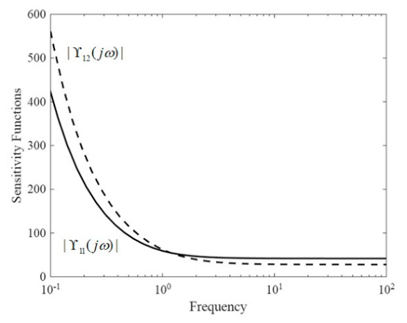
It is clear from (50) and (51) that the canonical basis axes of the system are rather sensitive to the variations Δ K 1 and Δ K 2 . The plots | ϒ 11 ( j ω ) | and | ϒ 12 ( j ω ) | are shown in Figure 6. From these plots and from (50) and (51), we see that the magnitudes of the sensitivity functions tend to infinity at zero frequency; i.e., the canonical basis axes are extremely sensitive to variations of the gains. At the same time, for the equal values and signs of Δ K 1 and Δ K 2 (i.e., for Δ K 1 = Δ K 2 ), the corresponding terms in (50) and (51) are mutually compensated, and in such situations the canonical basis does not depend at all on the variations Δ K 1 and Δ K 2 .
Finaly, consider the sensitivity of the CTFs of the closed-loop system. With the help of Formulae (37), it is easy to find
S 11 S ( s ) = 49 ( s + 1 ) ( s + 2 ) 2   ,           S 21 S ( s ) = 96 ( s + 2 ) ( s + 4 ) 2   ,       S 12 S ( s ) = 48 ( s + 1 ) ( s + 2 ) 2 ,             S 22 S ( s ) = 98 ( s + 2 ) ( s + 4 ) 2 .
Comparison of (52) and (47) shows that the introduction of feedback decreases the sensitivity of the CTFs to the variations Δ K 1 and Δ K 2 . Thus, at the zero frequency ω = 0 , these functions are equal to
S 11 S ( j 0 ) = 12.25 ,         S 21 S ( j 0 ) = 12 ,         S 12 S ( j 0 ) = 12 ,         S 22 S ( j 0 )   =   12.25 ,
i.e., the feedback decreases the sensitivity to variations Δ K 1 and Δ K 2 approximately by a factor of four. The magnitude plots | S 11 S ( j ω ) | and | S 12 S ( j ω ) | are shown in Figure 7 (two other plots practically coincide with the given in Figure 7). Note that the sensitivity functions of the CTFs of the closed-loop system have insignificant resonance peaks.
Hence, such extraordinary behavior of the discussed two-dimensional system in the case of small Δ K 1 and Δ K 2 is due to extremely high sensitivity to non-identical variations of these parameters. This becomes especially apparent if the variations have opposite signs.
The reason for all this is quite simple. As is known [15,16,17,18,19,20], the robustness of feedback systems depends on H norm of the transfer matrices S ( s ) or T ( s ) (3). Using, for example, the canonical Representation (6), we have
          S ( j ω ) = C ( j ω ) d i a g 1 1 + q i ( j ω ) C 1 ( j ω )                                   ν C ( j ω ) max i 1 1 + q i ( j ω ) ,
where
ν C ( j ω ) = C ( j ω ) C 1 ( j ω )
is the condition number of the modal matrix C ( j ω ) [3]. In general, the condition number is unity for orthogonal bases and tends to infinity if the axes of the basis approach to a linearly dependent reference frame. This means that the robustness of MIMO control systems deteriorates with an increase in the condition number ν C ( j ω ) (54).
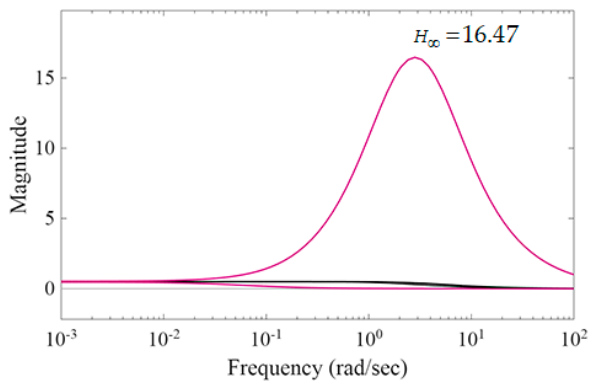
In this respect, the angle between the canonical bases axes of the System (41) is about 179.45°; that is, practically, the axes belong to the same line, and the condition number ν C (54) is equal to 196. The generalized frequency-response characteristics of the closed-loop system are shown in Figure 8 in vinous color. The exact value of H norm is 16.47. This indicates that the system is non-robust and the admissable norm of the additive perturbation is 0.061 (note that the norm of the regulator K (43) is 1.13).
In other words, the discussed example shows only that the System (40), but not the CTFs method, is not robust.

4.2. Control System of a Hexacopter

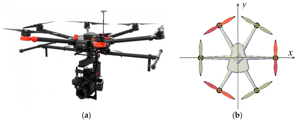
Consider the control system of the hexacopter shown in Figure 9. Generally, irrespective of the number of motors, the flight altitude z and the vector of rotation angles (roll ϕ , pitch θ , and yaw ψ ) are usually chosen as four control variables in UAVs’ control systems [37].
Below, we shall assume that the angles and angular velocities of the UAV are so small that nonlinear terms in the dynamics equations of rotational motions can be neglected, the cosines of all angles are approximately equal to one, and sines of the angles are zero. On these conditions, the dynamics equations of multirotor UAVs have the following linearized form [37,38]:
d 2 z ( t ) d t 2 = 1 m T Σ ( t ) g ,
J d ω ( t ) d t = τ ( t )
where m is the mass of the UAV; g the gravitational constant; J is diagonal tensor of inertia with the components I x ,   I y ,   I z on the principal diagonal; ω ( t ) is the vector of angular velocities in the body-fixed frame; vector τ ( t ) = [ τ x , τ y , τ z ] T combines the principal non-conservative forces and moments applied to the UAV airframe by the aerodynamics of the six rotors (assuming no external disturbances);
T Σ = i = 1 6 T i
the total thrust at hover, where T i is the thrust generated by the i th rotor (i = 1, 2, …, 6). Denoted by T ¯ , the 6-dimensional vector of thrusts T i ( T ¯ = [ T 1 , T 2 , , T 6 ] T ) and the mapping of T ¯ to the vector T Σ , τ T can be written in matrix form
T Σ τ = D M Λ M T ¯ ,       Λ M = d i a g λ i M .
In (58), the 4 × 6 full-rank numerical matrix D M for the motors allocation in Figure 9b is [39]
D M = 1 1 1 1 1 1 0 0.866 L 0.866 L 0 0.866 L 0.866 L L L / 2 L / 2 L L / 2 L / 2 k ψ k ψ k ψ k ψ k ψ k ψ ,
where L is the distance of the motors from the center of mass, k ψ is a design parameter of the motors [37], and λ i M   ( 0 < λ i M 1 ) (i = 1, 2, …, 6) are the motors efficiency degradation parameters. For properly functioning motors, the matrix Λ M is equal to 6 × 6 identity matrix I (or I 6 × 6 , to indicate the order of the matrix I ).
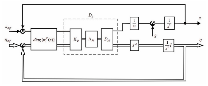
The matrix block diagram of the UAV’s control system is shown in Figure 10 [39].
Commonly, the matrix regulator K Reg ( s ) in such systems is taken in the form
K Reg ( s ) = K R d i a g { w i R ( s ) } ,
where K R is a constant matrix, and w i R ( s ) are scalar transfer functions of the regulators in the separate channels. Usually, standard proportional-integral-derivative (PID) regulators are used as w i R ( s ) in (60).
The transfer matrix of the open-loop control system of the hexacopter in Figure 10 has the form:
W ( s ) = 1 s 2 M 1 D M Λ M K R d i a g w i R ( s ) ,
where
M = m 0 0 0 0 I x 0 0 0 0 I y 0 0 0 0 I z .
The matrix K R in (60) and (61) is usually chosen as
K R = D M + M Σ ,
D M + = 1 / 6 1 / 6 1 / 6 1 / 6 1 / 6 1 / 6 3 / 6 L 3 / 6 L 3 / 6 L 0 3 / 6 L 3 / 6 L 1 / 3 L 1 / 6 L 1 / 6 L 3 / 6 L 1 / 6 L 1 / 6 L 1 / 6 k ψ 1 / 6 k ψ 1 / 6 k ψ 1 / 6 k ψ 1 / 6 k ψ 1 / 6 k ψ T ,
where T is the sign of matrix transposition, and D M + denotes the 6 × 4 Moore–Penrose pseudoinverse of the matrix D M (59) [37,38,39].
In what follows, we shall assume, for simplicity, that all regulators w i R ( s ) in (60) are identical, i.e., w i R ( s ) = w R ( s ) .
In the case of no motors’ efficiency degradations (i.e., if Λ M = I 6 × 6 ), we have M Σ 1 D M K R = I 4 × 4 ; i.e., the kinematic cross-connections between the four separate channels of the systems in Figure 10 are compensated, and the transfer matrix of the open-loop system reduces to the form
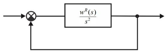
W ( s ) = w R ( s ) s 2 I 4 × 4 .
Correspondingly, the matrix block diagram in Figure 10 splits into four isolated SISO channels in Figure 11.
On the other hand, if there are some degradations of motors efficiency, i.e., if Λ M I 6 × 6 , then, instead of (61), we have
W ( s ) = w R ( s ) s 2 B Σ ,
where the matrix
B Σ = M 1 D M Λ M K R = M 1 D M Λ M D M + M
is not an identity matrix. Consequently, if Λ M I 6 × 6 , then the control system of the hexacopter belongs to the class of cross-connected MIMO control systems.
Let the parameters of the hexacopter in Equations (55) and (56) be: m = 2.5   kg , I x = I y = 0.5   kg m 2 , I z = 1.5   kg   ×   m 2 . The matrix M Σ (62), in this case, has the form
M = 2.5 0 0 0 0 0.5 0 0 0 0 0.5 0 0 0 0 1.5 .
The identical proportional-integral-derivative (PID) regulators with the first order filter w R ( s ) in the separate channels are taken in the form:
w R ( s ) = K P + K I s + K D s T f s + 1 ,
where K P = 0.1857 ,   K I = 0.008693 ,   K D =   0.9739 ,   T f 0.1834 . The parameters of the PID regulator (69) are obtained using the function pidtune in MATLAB [40].
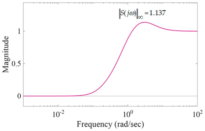
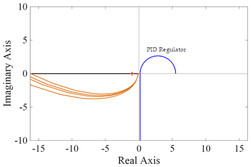
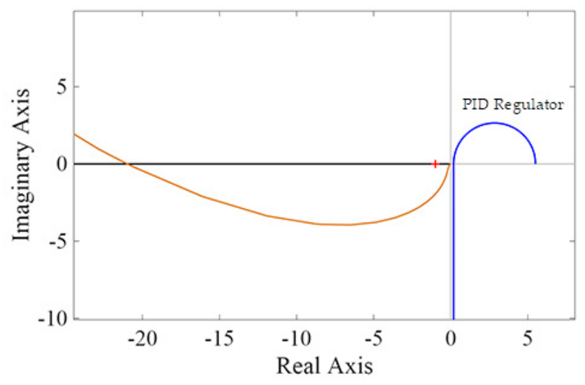
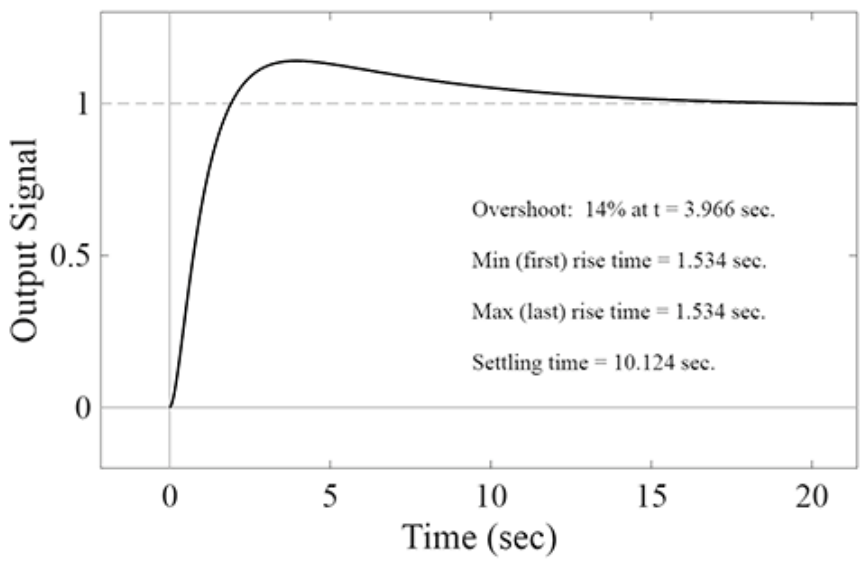
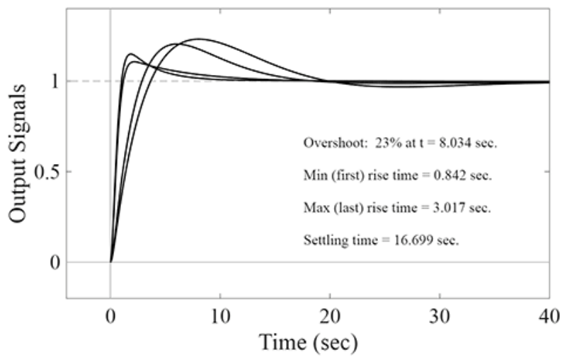
The frequency-response and step-response characteristics of the separate channels in the case of ideal motors (when Λ M = I 6 × 6 ) are shown in Figure 12, Figure 13 and Figure 14. In Figure 12, the black line is the graph of the plant (a double integrator), the blue line represents the PID regulator (69), and the transfer function of the resulting open-loop channel is shown by the brown line.
Let us now analyze the sensitivity of the hexacopter’s control system to small degradations of the motors efficiency, supposing that the matrix Λ M in (58) has the following form:
Λ M = 0.75 0 0 0 0 0 0 1.0 0 0 0 0 0 0 0.8 0 0 0 0 0 0 0.95 0 0 0 0 0 0 0.77 0 0 0 0 0 0 0.85 .
The matrix of cross-connections B Σ (67), in this case, is
B Σ = 0.853 0.010 0.004 0.160 0.130 0.855 0.017 0.173 0.050 0.017 0.852 0.017 0.040 0.004 0.00 0.853 ,
and the CTFs of the open-loop system are
q 1 ( s ) = 5.2355 ( s + 0.096 ) ( s + 0.0902 ) s 3 ( s + 5.453 ) q 2 ( s ) = 4.2319 ( s + 0.096 ) ( s + 0.0902 ) s 3 ( s + 5.453 ) q 3 ( s ) = 4.754 ( s + 0.096 ) ( s + 0.0902 ) s 3 ( s + 5.453 ) q 4 ( s ) = 4.5397 ( s + 0.096 ) ( s + 0.0902 ) s 3 ( s + 5.453 ) .
Due to the structural features of the control system, the modal matrix C ( s ) in (4) is constant; i.e., C ( s ) = C , and equal to
C = 0.410 0.623 0.056 0.023 0.891 0.490 0.508 0.824 0.018 0.541 0.860 0.563 0.196 0.280 0.016 0.064 .
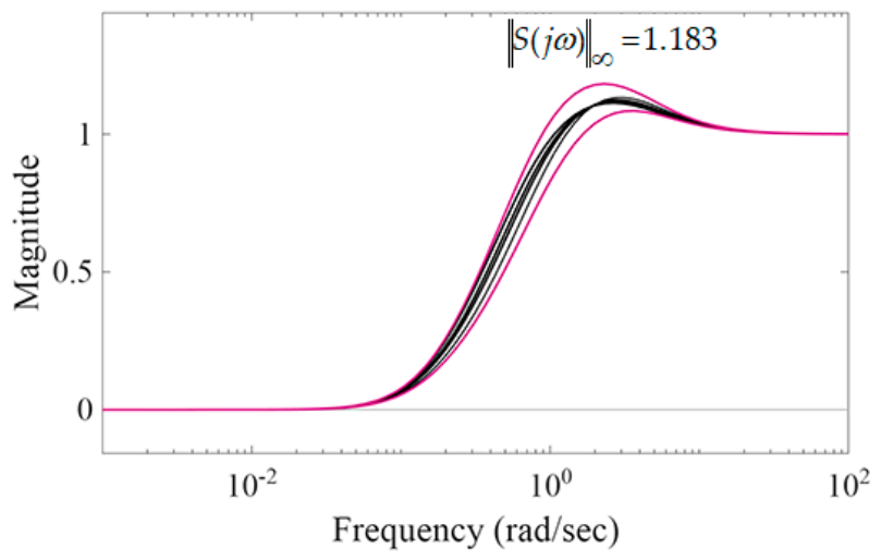
The Nyquist plot, generalized frequency responses and step response of the hexacopter’s control system with the motors degradation parameters given by the matrix Λ M (70) are shown in Figure 15, Figure 16 and Figure 17. In Figure 15, the four coinciding black lines are the graphs of the plant, the blue line represents the identical PID regulator (66) in the separate channels, and the gain loci of the CTFs (72) are shown by brown lines. The vinous lines in Figure 16 represent the majorant and minorant of the generalized frequency-response characteristics, and the black lines depict the sensitivity functions of the closed-loop characteristic systems.
Using Expressions (23), we obtain the following three matrices that determine the sensitivity of the CTFs and canonical basis axes to small efficiency degradations λ 1 M , λ 2 M , and λ 3 M of the first three motors:
N 1 ( s ) = 5.496 ( s + 0.096 ) ( s + 0.0902 ) s 3 ( s + 5.453 ) 0.17 0 0.07 0.33 0 0 0 0 0.83 0 0.33 1.67 0.08 0 0.03 0.17
N 2 ( s ) = 5.496 ( s + 0.096 ) ( s + 0.0902 ) s 3 ( s + 5.453 ) 0.17 0.06 0.03 0.33 0.72 0.25 0.14 1.44 0.42 0.14 0.08 0.83 0.08 0.03 0.02 0.17
N 3 ( s ) = 5.496 ( s + 0.096 ) ( s + 0.0902 ) s 3 ( s + 5.453 ) 0.17 0.06 0.03 0.33 0.72 0.25 0.14 1.44 0.42 0.14 0.08 0.83 0.08 0.03 0.02 0.17
Due to the symmetry of the motors allocations, the matrices N 4 ( s ) , N 5 ( s ) , and N 6 ( s ) for other three motors are actually equal in pairs (up to the signs of non-diagonal terms) to matrices (74)–(76).
These expressions, together with (35), (37) and (39), can be used for analyzing sensitivity of the hexacopter control systems with respect to variations of the parameters of motors, sensors, regulators, etc.

5. Discussion and Conclusions

In this paper, the problem of sensitivity of multivariable control systems is analyzed within the framework of the CTFs method. The formulas determining the sensitivity functions of the CTFs and sensitivity vectors of the canonical basis axes to small variations of parameters of general type MIMO control systems are derived. The relations between the sensitivity functions of open-loop and closed-loop MIMO systems are established. It is shown that the sensitivity functions of the CTFs of the open-loop and the closed-loop MIMO systems are related to each other by the same expressions as the standard sensitivity functions of the open-loop and closed- loop SISO systems. Furthermore, the sensitivity vectors of the canonical basis axes are not affected by the introduction of feedback loop.
In future research, it is intended to extend the results of the paper to special structural classes of MIMO control systems, such as uniform system, symmetric systems, anti-symmetric systems, etc.
It should be noted that the CTFs method was successfully used in aerospace engineering, particularly in the design of high-precision guidance systems of two astronomical telescopes mounted on the space station “MIR”. Nevertheless, in the technical literature on multivariable feedback control, that method is often claimed to be not robust and, therefore, unreliable in practical design. That erroneous conclusion has become quite common because of two main reasons.
First, it is due to the notorious example usually attributed to J. Doyle and G. Stein [24], where it is shown that a two-dimensional system having, at first glance, infinite gain margins calculated through the CTFs becomes unstable in the case of small additive perturbations of the controller’s gains. In this paper, a detailed analysis of the sensitivity and robustness of the system in [24] is given, and it is shown that the incorrect conclusion about robustness was made because of improper application of the CTFs method (improper treatment of the results). In short, the example in [24] can be considered as an equally good illustrative example of a non-robust control system but not evidence of unreliability of the CTFs method. The point is that the robustness of MIMO control systems essentially depends not only on stability margins of the SISO characteristic systems but also on the skewness of the canonical basis axes (or condition number of the modal matrix), which, in this case, is quite close to critical.
The second reason is more significant. The design of MIMO control systems is computationally intensive and cannot be performed without specialized computer-aided control system design (CACSD) tools [40,41,42,43,44,45]. Unfortunately, at present, there are no acknowledged CACSD tools based on the CTFs method. It is worth mentioning that in the 1990s, the Multivariable Frequency-Domain Toolbox (MFD Toolbox) was developed by J.M. Maciejowski, M.P. Ford, and J.B. Boyle at Cambridge Control Ltd. [46]. The MATLAB-based MFD Toolbox was designed for the analysis and design of linear MIMO systems. Among some other design techniques, the MFD Toolbox supported also the CTFs method for both continuous-time and discrete-time systems. However, no information can be found about the current situation with that toolbox.
In this respect, a new software package, called MIMO Control Toolbox, is being developed at the Aerial Robotics Center of the National Polytechnic University of Armenia [47]. The toolbox works in the MATLAB environment and is designed for analysis and design of control systems in robotics, mechatronics, and many other fields. The principal feature of the MIMO Control Toolbox is that the design of any N-dimensional MIMO control system is reduced to the design of a certain fictitious SISO control system. Another key feature of the toolbox is that it includes about 250 new MATLAB classes (objects) describing all the main structural types of MIMO control systems known from the scientific and technical literature.
The frequency and time-response characteristics of the hexacopter’s control system in Figure 12, Figure 13, Figure 14, Figure 15, Figure 16 and Figure 17 were obtained with the help of a special interactive graphical user interface (GUI) which is a part of the MIMO Control Toolbox package and which can be viewed as an extension to the multivariable case of the well-known GUI Control Systems Designer in MATLAB [40]. The MIMO Control Toolbox can be used both as a computer-aided control systems design tool in industry and various engineering applications and for teaching the fundamentals of classical and modern feedback control at educational institutions.


Author Contributions

Conceptualization, O.G., N.N., L.B. and K.B.; methodology, O.G., N.N. and L.B.; software, O.G., D.D., M.H. and K.B.; validation, O.O., M.D., D.D., M.H. and K.B.; formal analysis, D.D., M.H. and K.B.; investigation, O.G., N.N., L.B., D.D. and M.H.; data curation, O.O., M.D. and K.B.; writing—original draft preparation, O.G. and L.B.; writing—review and editing, O.G. and L.B.; visualization, L.B., O.O. and M.D.; supervision, O.G.; project administration, O.G. and L.B.; All authors have read and agreed to the published version of the manuscript.

Funding

This research received no external funding.

Data Availability Statement

The original contributions presented in this study are included in the article. Further inquiries can be directed to the corresponding author.

Conflicts of Interest

The authors declare no conflicts of interest.

Abbreviations

The following abbreviations are used in this manuscript:
CACSDComputer-aided control system design
GUIGraphical user interface
MIMOMulti-input multi-output
PIDProportional-integral-derivative
SISOSingle-input single-output
UAVUnmanned aerial vehicle

References

  1. Skogestad, S.; Postlethwaite, I. Multivariable Feedback Control: Analysis and Design, 2nd ed.; Wiley-Interscience: Oxford, UK, 2005; 592p. [Google Scholar]
  2. Maciejowski, J.M. Multivariable Feedback Design; Addison-Wesley Longman Publishing Company: Boston, MA, USA, 1989; 448p. [Google Scholar]
  3. Gasparyan, O.N. Linear and Nonlinear Multivariable Feedback Control: A Classical Approach; John Wiley & Sons: Bognor Regis, UK, 2008; 341p. [Google Scholar]
  4. Iqbal, U.; Samad, A.; Nissa, Z.; Iqbal, J. Embedded control system for AUTAREP—A novel AUTonomous Articulated Robotic Educational Platform. Teh. Vjesn.-Tech. Gaz. 2014, 21, 1255–1261. [Google Scholar]
  5. Horowitz, I.M. Synthesis of Feedback Systems; Academic Press: New York, NY, USA, 1963; 726p. [Google Scholar]
  6. Tomovic, R.; Vulkobratovic, M. General Sensitivity Theory; Elsevier: Amsterdam, The Netherlands, 1972; 258p. [Google Scholar]
  7. Eslami, M. Theory of Sensitivity in Dynamic Systems: An Introduction; Springer: Berlin, Germany, 1994; 601p. (In English) [Google Scholar]
  8. Rozenvasser, E.N.; Yusupov, R.M. Sensitivity of Automatic Control Systems, 1st ed.; CRC Press: Boca Raton, FL, USA, 1999; 456p. [Google Scholar] [CrossRef]
  9. Cruz, J.; Perkins, W. A new approach to the sensitivity problem in multivariable feedback system design. IEEE Trans. Autom. Control 1964, 9, 216–223. [Google Scholar] [CrossRef]
  10. Morgan, B. Sensitivity analysis and synthesis of multivariable systems. IEEE Trans. Autom. Control 1966, 11, 506–512. [Google Scholar] [CrossRef]
  11. Dooren, P.V. The generalized eigenstructure problem in linear system theory. IEEE Trans. Autom. Control 1981, 26, 111–129. [Google Scholar] [CrossRef]
  12. Kazlauskas, K. Sensitivity Analysis of Multivariable Systems in State Space. Informatica 2000, 11, 97–110. [Google Scholar] [CrossRef]
  13. Bestle, D. Eigenvalue sensitivity analysis based on the transfer matrix method. Int. J. Mech. Syst. Dyn. 2021, 1, 96–107. [Google Scholar] [CrossRef]
  14. Dorf, R.C.; Bishop, R.H. Modern Control Systems, 14th ed.; Pearson: London, UK, 2022; 1032p. [Google Scholar]
  15. Zhou, K.; Doyle, J.C. Essentials of Robust Control; Prentice Hall: Upper Saddle River, NJ, USA, 1998; 432p. [Google Scholar]
  16. Zhou, K.; Doyle, J.C.D.; Glover, K. Robust and Optimal Control; Prentice Hall: Upper Saddle River, NJ, USA, 1995; 616p. [Google Scholar]
  17. Green, M.; Limebeer, D.J.N. Linear Robust Control; Prentice Hall: Englewood Cliffs, NJ, USA, 1995; 538p. [Google Scholar]
  18. Dullerud, G.E.; Paganini, F. A Course in Robust Control Theory: A Convex Approach; Springer: Berlin/Heidelberg, Germany, 2010; 439p. [Google Scholar]
  19. Ackermann, J. Robust Control: Systems with Uncertain Physical Parameters; Springer: New York, NY, USA, 1993; 406p. [Google Scholar]
  20. Yan, Y.; Xu, P.; Yue, J.; Chen, Z. Robust Control: From Continuous-State Systems to Finite State Machines. IEEE Trans. Autom. Sci. Eng. 2024, 21, 2156–2163. [Google Scholar] [CrossRef]
  21. Astrom, K.J.; Wittenmark, B. Adaptive Control, 2nd ed.; Addison-Wesley: Boston, MA, USA, 1994; 580p. [Google Scholar]
  22. Kirk, D.E. Optimal Control Theory: An Introduction; Dover Publications: Garden City, NY, USA, 2004; 480p. [Google Scholar]
  23. Rawlings, J.; Mayne, D.Q.; Diehl, M. Model Predictive Control: Theory, Computation, and Design; Nob Hill Pub, LLC: Portland, OR, USA, 2017; 533p. [Google Scholar]
  24. Doyle, J.; Stein, G. Multivariable feedback design: Concepts for a classical/modern synthesis. IEEE Trans. Autom. Control 1981, 26, 4–16. [Google Scholar] [CrossRef]
  25. Safonov, M.G. Stability and Robustness of Multivariable Feedback System; MIT Press: Cambridge, MA, USA, 1980; 171p. [Google Scholar]
  26. Macfarlane, A.G.J.; Belletrutti, J.J. The characteristic locus design method. Automatica 1973, 9, 575–588. [Google Scholar] [CrossRef]
  27. MacFarlane, A.G.J.; Postlethwaite, I. Characteristic frequency functions and characteristic gain functions. Int. J. Control 1977, 26, 265–278. [Google Scholar] [CrossRef]
  28. MacFarlane, A.G.J.; Kouvaritakis, B. A design technique for linear multivariable feedback systems. Int. J. Control 1977, 25, 837–874. [Google Scholar] [CrossRef]
  29. MacFarlane, A.G.J. Commutative controller: A new technique for the design of multivariable control systems. Electron. Lett. 1970, 6, 121–123. [Google Scholar] [CrossRef]
  30. Postlethwaite, I. Sensitivity of the characteristic gain loci. Automatica 1982, 18, 709–712. [Google Scholar] [CrossRef]
  31. Moreira, M.V.; Basilio, J.C. Characteristic locus method robustness improvement through optimal static normalizing pre-compensation. Int. J. Robust. Nonlinear Control 2010, 20, 371–386. [Google Scholar] [CrossRef]
  32. Razavi, S.; Jakeman, A.; Saltelli, A.; Prieur, C.; Iooss, B.; Borgonovo, E.; Plischke, E.; Piano, S.L.; Iwanaga, T.; Becker, W.; et al. The future of sensitivity analysis: An essential discipline for systems modeling and policy support. Environ. Model. Softw. 2021, 137, 104954. [Google Scholar] [CrossRef]
  33. Todorov, V.; Zhivkov, P. Efficient Evaluation of Sobol’ Sensitivity Indices via Polynomial Lattice Rules and Modified Sobol’ Sequences. Mathematics 2025, 13, 3402. [Google Scholar] [CrossRef]
  34. Díaz-Zurita, A.; Naval-Hernández, V.M.; Whiteman, D.N.; Rodríguez-Navarro, O.; Muñiz-Rosado, J.; Pérez-Ramírez, D.; Alados-Arboledas, L.; Navas-Guzmán, F. Sensitivity Analysis of the Differential Atmospheric Transmission in Water Vapour Mixing Ratio Retrieval from Raman Lidar Measurements. Remote Sens. 2025, 17, 3444. [Google Scholar] [CrossRef]
  35. Gelfand, I.M. Lectures on Linear Algebra; Dover Publications, No. 1; Interscience Publishers: New York, NY, USA, 1989; 208p. [Google Scholar]
  36. Tosio, K. Perturbation Theory for Linear Operators; Grundlehren der Mathematischen Wissenschaften: A Series of Comprehensive Studies in Mathematics; Springer: Berlin/Heidelberg, Germany, 2012; 643p. [Google Scholar]
  37. Mahony, R.; Kumar, V.; Corke, P. Multirotor Aerial Vehicles: Modeling, Estimation, and Control of Quadrotor. IEEE Robot. Autom. Mag. 2012, 19, 20–32. [Google Scholar] [CrossRef]
  38. Irfan, S.; Zhao, L.; Ullah, S.; Javaid, U.; Iqbal, J. Differentiator- and Observer-Based Feedback Linearized Advanced Nonlinear Control Strategy for an Unmanned Aerial Vehicle System. Drones 2024, 8, 527. [Google Scholar] [CrossRef]
  39. Gasparyan, O.N.; Darbinyan, H.G. Adaptive System of Compensation of Motors’ Partial Degradations of Multirotor UAVs. In Modern Problems of Robotics; Yuschenko, A., Ed.; Springer International Publishing: Cham, Switzerland, 2021; pp. 207–219. [Google Scholar] [CrossRef]
  40. Control System Toolbox User’s Guide; MathWorks: South Natick, MA, USA, 2025; 1936p.
  41. Linkens, D.A. CAD for control systems—A review of PC software. Comput.-Aided Des. 1988, 20, 564–565. [Google Scholar] [CrossRef]
  42. Gasparyan, O.N. Computer-aided analysis and design of linear and nonlinear multivariable control systems: A classical approach. In Proceedings of the 2006 IEEE Conference on Computer Aided Control System Design, Munich, Germany, 4–6 October 2006; pp. 1958–1963. [Google Scholar] [CrossRef]
  43. Blackwell, C.; Sastry, M.K.S. Multivar—A MATLAB Based MIMO Control System Design Application. In Proceedings of the 2016 8th International Conference on Computational Intelligence and Communication Networks (CICN), Tehri, India, 23–25 December 2016; pp. 318–323. [Google Scholar] [CrossRef]
  44. Balas, G.J.; Chiang, R.Y.; Packard, A.; Safonov, M.G. Robust Control Toolbox™ User’s Guide; MathWorks, Inc.: Natick, MA, USA, 2025. [Google Scholar]
  45. Bemporad, A.; Morari, M.; Ricker, N.L. Model Predictive Control Toolbox™ Getting Started Guide; MathWorks, Inc.: Natick, MA, USA, 2025; 986p. [Google Scholar]
  46. Maciejowski, J.M. The multivariable frequency domain toolbox and its relation to other MATLAB toolboxes. In Proceedings of the International Conference on Control 1991. Control ’91, Edinburgh, UK, 25–28 March 1991; Volume 1, pp. 471–475. [Google Scholar]
  47. Gasparyan, O.N.; Simonyan, T.A.; Buniatyan, L.M.; Karapetyan, A.K. A new toolbox for computer-aided analysis and design of multivariable control systems in robotics and mechatronics. SSRG Int. J. Electr. Electron. Eng. 2026, 13, 169–177. [Google Scholar] [CrossRef]
Figure 1. Block-diagram of a MIMO control system.
Automation 07 00089 g001
Figure 2. Canonical representation of the open-loop MIMO system.
Automation 07 00089 g002
Figure 3. Canonical representation of the closed-loop MIMO system.
Automation 07 00089 g003
Figure 4. Stability analysis of a two-dimensional system (41): (a) CTFs in case of the unit regulator K = I ; (b) CTFs in case of the perturbed regulator K (43).
Automation 07 00089 g004
Figure 5. Sensitivity functions | S 11 q ( j ω ) | and | S 12 q ( j ω ) | .
Automation 07 00089 g005
Figure 6. Sensitivity functions | ϒ 11 ( j ω ) | and | ϒ 12 ( j ω ) | .
Automation 07 00089 g006
Figure 7. Sensitivity functions | S 11 S ( j ω ) | and | S 12 S ( j ω ) | .
Automation 07 00089 g007
Figure 8. Generalized frequency responses of the closed-loop system.
Automation 07 00089 g008
Figure 9. Hexacopter: (a) general view; (b) motors’ allocation.
Automation 07 00089 g009
Figure 10. Matrix block diagram of the UAV’s control system.
Automation 07 00089 g010
Figure 11. Block diagram of isolated separate channels in case of ideal motors ( Λ M = I 6 × 6 ).
Automation 07 00089 g011
Figure 12. Nyquist plots of the isolated channels ( Λ M = I 6 × 6 ).
Automation 07 00089 g012
Figure 13. Frequency-response characteristic of the sensitivity function of the isolated channels ( Λ M = I 6 × 6 ).
Automation 07 00089 g013
Figure 14. Step response of the isolated channels ( Λ M = I 6 × 6 ).
Automation 07 00089 g014
Figure 15. Nyquist plots of the CTFs ( Λ M I 6 × 6 ).
Automation 07 00089 g015
Figure 16. Generalized frequency-response characteristics of the sensitivity function matrix.
Automation 07 00089 g016
Figure 17. Step responses of the control system ( Λ M I 6 × 6 ).
Automation 07 00089 g017
Disclaimer/Publisher’s Note: The statements, opinions and data contained in all publications are solely those of the individual author(s) and contributor(s) and not of MDPI and/or the editor(s). MDPI and/or the editor(s) disclaim responsibility for any injury to people or property resulting from any ideas, methods, instructions or products referred to in the content.