Optimizing Unmanned Air–Ground Vehicle Maneuvers Using Nonlinear Model Predictive Control and Moving Horizon Estimation

Abstract

In this paper, Nonlinear Model Predictive Control (NMPC) and Nonlinear Moving Horizon Estimator (NMHE) are combined to control, in a distributed way, a heterogeneous fleet composed of a steering car and a quadcopter. In particular, the ground vehicle in the role of the leader communicates its one-step future position to the drone, which keeps the formation along the desired trajectory. Inequality constraints are introduced in a switching control fashion to the leader’s NMPC formulation to avoid obstacles. In the literature, few works using NMPC and NMHE deal with these two vehicles together. Moreover, the presented scheme can tackle noisy, partial, and missing measurements of the agents’ state. Results show that the ground car can avoid detected obstacles, keeping the tracking errors of both robots in the order of a few centimeters, thanks to trustworthy NMHE estimates and NMPC predictions.

1. Introduction

Multiple robot systems have become widespread, as they can perform hard and possibly dangerous tasks for humans while improving efficiency and productivity. Among the plethora of applications, there are industry, agriculture, construction, and emergency rescue [1].

Among the different kinds of collaboration, hybrid teams can tackle more complex tasks requiring different capabilities, notably air–ground cooperation. On the one hand, Unmanned Aerial Vehicles (UAVs) have long-range sensors on board, making them suitable for monitoring from the sky. On the other side, Unmanned Ground Vehicles (UGVs) have short-range sensors and high load and computational capacities. The main issues are motion control, formation control, and collision avoidance. Vinicius et al. [2] proposed a light path following a virtual structure-based controller for package delivery. As the UAV flies over it, the UGV has to follow a desired trajectory while avoiding obstacles.

A PI optimal control theory is presented in [3], and results show that the proposed scheme can overcome input and model disturbances and linearization biases. Again considering air–ground cooperation, ref. [4] presents a leader–follower architecture, where the quadcopter has to reach the desired waypoints and send its position to the unicycle, which uses these data as the desired position. In addition, the ground agent should avoid obstacles around it.

Classical control methods assume complete knowledge of the system state without data loss. When agents are not tracked, the control action cannot be computed, and the robots must halt. Nonlinear Model Predictive Control (NMPC) provides a solution to this issue. In the absence of measurements, NMPC can apply the optimal control trajectory computed in the previous step until updated data become available. The key idea is to use an internal nonlinear model to predict the system’s future response. Due to its simplicity, MPC has been widely used in various applications, with numerous studies experimentally validating its superiority over classical linear controllers. In [5], the authors compared the performance of PID, LQR and MPC in controlling a drone. Both simulations and real experiments with a Parrot mini-drone were carried out. It turns out that MPC outperforms other methods, ensuring robustness, stability, and small errors in terms of maximum pitch deviation. Al-Saoudi et al. [6] carried out a similar study comparing model-based controllers such as PID, fuzzy logic, and MPC with an ANFIS-based controller. From the MATLAB/SIMULINK R2022a tests, it is shown that the MPC is superior, as it can handle input constraints and has lower overshoot and response time compared to other techniques. Taking into account a separation clutch system in the slipping state, ref. [7] compares PI-PD and LQR methods with a scheme composed of multiple MPCs but again this last turns out to be the best in terms of performance. Always in the field of autonomous driving, the paper [8] studies and evaluates in terms of tracking error different methods (Pure Pursuite, Stanley, LQR and MPC) for the trajectory tracking mission of a steering car. In both tests, MPC provides better accuracy both for the eight shape and the circle path. While NMPC has been consolidated over the years for controlling UGVs, leading to embedded implementations [9,10], it has been applied to UAVs only recently. Indeed, with the advent of more powerful microprocessors and efficient nonlinear solvers, a real-time application of NMPC for small drones is now possible [11].

However, one of the primary limitations of NMPC is the assumption that the complete state is measurable. To overcome this, NMPC is often paired with nonlinear estimators, such as the Nonlinear Moving Horizon Estimator (NMHE) [12]. NMHE addresses the dual problem of NMPC by providing state estimates that incorporate constraints and nonlinearities without assuming a specific error distribution. This pairing allows NMPC to function effectively even when full state information is not directly measurable. These two complementary state-of-the-art tools, when combined, can accurately control and estimate complex underactuated systems. In [13], the authors propose an NMHE-NMPC scheme to address the path-following problem of generalized N-vehicles under noisy measurements and disturbances. To evaluate its performance, simulations and real-world experiments have been performed to show its accuracy and applicability to real-time scenarios. A combination of both techniques is presented in [14] to control a selective catalytic reduction process for reducing engine emissions. In the context of UAVs, ref. [15] proposes a new NMPC method for UAV navigation that can deal with dynamic obstacles by predicting their movement and using a fast solver to find safe trajectories in real time, while [16] presents a nonlinear fault-tolerant control system for a quadcopter. This approach combines NMPC and NMHE to maintain trajectory control even in the presence of rotor failures. In the worst-case scenario where all motors are damaged, the NMHE estimates allow the NMPC to effectively stabilize and accurately follow the reference trajectory.

This work addresses the UAV-UGV formation and path-tracking problem. In particular, a distributed leader–follower NMPC-NMHE scheme is defined. The main novelties and contributions of this paper are the following:

(a)

Although promising results have been obtained in various applications, NMPC and NMHE have not been used together for air–ground cooperation.

(b)

To the best of the authors’ knowledge, these two receiving horizon techniques have not been used to control a heterogeneous fleet consisting of a steering car and a quadcopter. In fact, most current work considers unicycles as ground vehicles.

(c)

It is worth noting that the proposed solution deals with partially noisy state measurements and is, in principle, robust to information loss.

The paper unfolds in three key sections. Section 2 outlines the methods and definitions devised to tackle the focal problem under examination. Moving forward, Section 3 consolidates the numerical simulation results. Ultimately, Section 4 encapsulates the conclusions, emphasizing future avenues for development.

2. Materials and Methods

The following sections will introduce the mathematical models employed in the problem formulation. Even if the UAV and the UGV present different dynamics, an NMPC and an NMHE have been developed for both agents. Moreover, it is assumed that the steering car communicates to the drone the one-step prediction of its state.

2.1. UAV and UGV Models

For describing the drone dynamics, the model defined in [17] is used.

$$\left\{\begin{array}{cc}\dot{x_1}\hfill & =x_2\hfill \\ \dot{x_2}\hfill & =-u_{1}sin\left({\theta }_1\right)/M\hfill \\ \dot{y_1}\hfill & =y_2\hfill \\ \dot{y_2}\hfill & =u_{1}cos\left({\theta }_1\right)sin\left({\varphi }_1\right)/M\hfill \\ \dot{z_1}\hfill & =z_2\hfill \\ \dot{z_2}\hfill & =u_{1}cos\left({\theta }_1\right)cos\left({\varphi }_1\right)/M-g\hfill \\ \dot{{\theta }_1}\hfill & ={\theta }_2\hfill \\ \dot{{\theta }_2}\hfill & =u_2\hfill \\ \dot{{\varphi }_1}\hfill & ={\varphi }_2\hfill \\ \dot{{\varphi }_2}\hfill & =u_3\hfill \\ \dot{{\psi }_1}\hfill & ={\psi }_2\hfill \\ \dot{{\psi }_2}\hfill & =u_4\hfill \end{array}\right.$$

(1)

The state variables are defined according to Figure 1. Hereinafter, let the state and control variables of the UAV at time t be denoted as:

$$\begin{array}{cc}\hfill {\mathit{x}}_{UAV}=& {\left[\begin{array}{cccccccccccc}{x}_1& x_2& y_1& y_2& z_1& z_2& {\theta }_1& {\theta }_2& {\varphi }_1& {\varphi }_2& {\psi }_1& {\psi }_2\end{array}\right]}^T\hfill \end{array}$$

(2)

$${\mathit{u}}_{UAV}={\left[\begin{array}{cccc}{u}_1& u_2& u_3& u_4\end{array}\right]}^T$$

(3)

and rewrite Equation (1) in a vectorial form

$${\dot{\mathit{x}}}_{UAV}=f_{UAV}({\mathit{x}}_{UAV},{\mathit{u}}_{UAV})$$

(4)

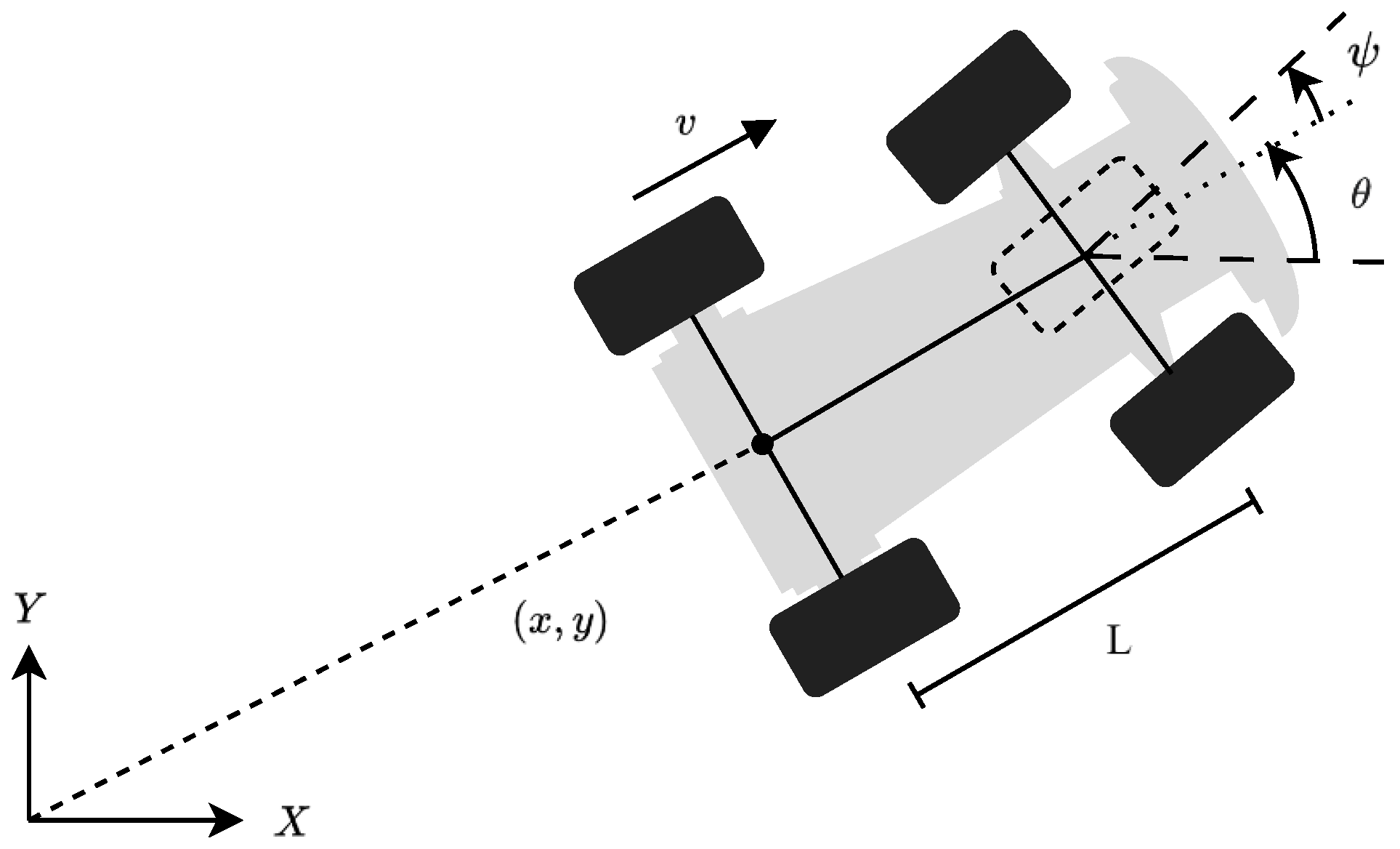
To study the steering car, the Ackermann model is used [18]. All the state quantities of the ground vehicle of the ground robot are depicted in Figure 2. The control variables are the steering angle $w_1\left(t\right)$ and the forward acceleration $w_2\left(t\right)$. The evolution model is

$$\left\{\begin{array}{cc}\dot{x}\hfill & =vcos\left(\theta \right)\hfill \\ \dot{y}\hfill & =vsin\left(\theta \right)\hfill \\ \dot{\theta }\hfill & =(v/L)tan\left(w_1\right)\hfill \\ \dot{v}\hfill & =w_2\hfill \end{array}\right.$$

(5)

The remainder of this paper will make use of the following notation:

$${\mathit{x}}_{UGV}={\left[\begin{array}{cccc}x& y& \theta & v\end{array}\right]}^T$$

(6)

$${\mathit{u}}_{UGV}={\left[\begin{array}{cc}{w}_1& w_2\end{array}\right]}^T$$

(7)

Thus, Equation (5) becomes

$${\dot{\mathit{x}}}_{UGV}=f_{UGV}({\mathit{x}}_{UGV},{\mathit{u}}_{UGV})$$

(8)

2.2. UAV NMPC

The drone’s NMPC aims to find the optimal control input to be applied by solving an optimization problem. Given the current estimated quadcopter’s state ${\widehat{\mathit{x}}}_{UAV}\left(k\right)$, the objective is to minimize the deviations from the reference $r_{UAV}\left(k\right)$ over a prediction horizon $H_p$ weighted by ${\mathcal{Q}}_{UAV}$. To predict the future behavior of the UAV, the discrete-time evolution $f_{UAV}$ is used, obtained by discretizing Equation (4) with sampling time $T_s$ and applying a trapezoidal rule:

$$\begin{array}{cc}\hfill min& \sum _{i=1}^{H_p}{∥{\mathit{x}}_{UAV}(k+i|k)-{\mathit{r}}_{UAV}\left(k\right)∥}_{{\mathcal{Q}}_{UAV}}^2\hfill \end{array}$$

(9a)

$$\begin{array}{cc}\hfill \mathrm{s}.\mathrm{t}.& {\mathit{x}}_{UAV}\left(k\right|k)={\widehat{\mathit{x}}}_{UAV}\left(k\right)\hfill \end{array}$$

(9b)

$$\begin{array}{c}\hfill \begin{array}{cc}\hfill & {\mathit{x}}_{UAV}(k+i+1|k)=\hfill \\ \hfill & f_{UAV}({\mathit{x}}_{UAV}(k+i|k),{\mathit{u}}_{UAV}(k+i|k))\hfill \end{array}\end{array}$$

(9c)

$$\begin{array}{cc}\hfill & x_{UAV}^{min}\le {\mathit{x}}_{UAV}(k+i|k)\le x_{UAV}^{MAX}\hfill \end{array}$$

(9d)

The decision variables are the state and the input trajectory, respectively $x_{UAV}(k+i|k)$ and $u_{UAV}(k+i|k)$, over the time window. To reduce the computational effort, it is assumed that after $H_u$ steps, the control remains constant. Regarding the reference, the drone should track the future position of the leader over the prediction horizon. Here, the trajectory is approximated with the future pose at the next step $k+1$ obtained by the car’s NMPC (see Section 2.5):

$$\begin{array}{cc}\hfill {\mathit{r}}_{UAV}\left(k\right)& =\left[\begin{array}{cccccc}x(k+1|k)& 0& y(k+1|k)& 0& z_{1,Ref}\left(k\right)& 0\end{array}\right.\hfill \\ \hfill & \hspace{1em}{\left.\begin{array}{cccccc}0& 0& 0& 0& \theta (k+1|k)& 0\end{array}\right]}^T\hfill \end{array}$$

(10)

Constraint Equation (9d) represents the structural limitations inherent to the drone’s design.

Conceptually, it is important to verify that the controller is stable and provides a control law that does not diverge, regardless of the system’s objective. Although the proof of stability is not included in this work, readers interested in a generalization may refer to Theorem 3 of [19], which is largely similar to the proposed theorem in this work, with the exception of minor constraints that are reasonably assumed not to affect the system’s stability. This is supported by the results in Section 3, which empirically confirm the validity of the control architecture for the proposed scenarios.

2.3. MHE for the UAV

The defined NMPC assumes that all state variables are known. However, some quantities cannot be measured directly, necessitating the introduction of an estimator, such as the MHE, which can deal with the exact nonlinear model and state and control boundaries. Taking into account a set of past noisy measurements,

$$\mathit{y}(k-i)i=0,\cdots ,H_e$$

(11)

and control inputs

$$\mathit{u}(k-i)i=0,\cdots ,H_e$$

(12)

over an estimation horizon $H_e$, the estimated state trajectory over the time window

$$\widehat{\mathit{x}}(k-i)i=0,\cdots ,H_e$$

(13)

is obtained by solving a constrained nonlinear optimization problem that penalizes the variations of the predicted measurement from the actual past values. Once the sequence of estimates is obtained, only the final value is retained, and the estimation horizon is shifted forward to repeat the computations at the next instant $k+1$. It is important to note that although the focus here is on nonmeasurable quantities, this technique can also be employed to estimate unknown parameters.

For a generic unmanned vehicle, the equations are

$$\begin{array}{cc}\hfill min& \sum _{i=1}^{H_e}{∥\mathit{y}(k-i)-h(\widehat{\mathit{x}}(k-i),\mathit{u}(k-i))∥}_{𝒱}^2\hfill \end{array}$$

(14a)

$$\begin{array}{cc}\hfill \mathrm{s}.\mathrm{t}.& \widehat{\mathit{x}}(k-i+1)=f(\widehat{\mathit{x}}(k-i),\mathit{u}(k-i))\hfill \end{array}$$

(14b)

$$\begin{array}{cc}\hfill & {\mathit{x}}_{UV}^{min}\le \widehat{\mathit{x}}(k-i)\le {\mathit{x}}_{UV}^{MAX}\hfill \end{array}$$

(14c)

where f and h are, respectively, the evolution and the measurement models. When considering a Gaussian measurement noise

$$\nu \left(t\right)\sim \mathcal{N}(0_{n_y\times 1},{\Sigma }_{\nu }){\Sigma }_{\nu }=\mathrm{diag}\left(\begin{array}{ccc}{\sigma }_1^2& \cdots & {\sigma }_{n_y}^2\end{array}\right)$$

(15)

the weighting matrix $𝒱$ is chosen as

$$𝒱={\left(\sqrt{{\Sigma }_{\nu }}\right)}^{-1}=\mathrm{diag}\left(\begin{array}{ccc}1/{\sigma }_1& \cdots & 1/{\sigma }_{n_y}\end{array}\right)$$

(16)

In the case of the quadcopter, $\widehat{\mathit{x}}(k-i)$ and $\mathit{u}(k-i)$ are, respectively, the estimate of the state ${\mathit{x}}_{UAV}$ and the control ${\mathit{u}}_{UAV}$ at instant $k-i$, $i=0,\cdots ,H_e$. It is reasonable to assume that a motion capture system can measure the pose of the robot with high accuracy. Although the Euler angles are defined in the body frame, a rotation matrix from the global reference frame can be defined. However, although this aspect is not addressed in the current context, measurement noise should be considered when developing an embedded system:

$${\nu }_{UAV}\left(t\right)\sim \mathcal{N}(0_{6\times 1},{\Sigma }_{{\nu }_{UAV}})$$

(17a)

$${\Sigma }_{{\nu }_{UAV}}=\mathrm{diag}\left(\left[\begin{array}{cccccc}{\sigma }_{x_1}^2& {\sigma }_{y_1}^2& {\sigma }_{z_1}^2& {\sigma }_{{\theta }_1}^2& {\sigma }_{{\varphi }_1}^2& {\sigma }_{{\psi }_1}^2\end{array}\right]\right)$$

(17b)

$$\begin{array}{cc}\hfill {𝒱}_{UAV}=& \mathrm{diag}\left(\left[\begin{array}{cccccc}1/{\sigma }_{x_1}& 1/{\sigma }_{y_1}& 1/{\sigma }_{z_1}& 1/{\sigma }_{{\theta }_1}& 1/{\sigma }_{{\varphi }_1}& 1/{\sigma }_{{\psi }_1}\end{array}\right]\right)\hfill \end{array}$$

(18)

$$h_{UAV}(\widehat{\mathit{x}}(k-i),\mathit{u}(k-i))=C_{UAV}\widehat{\mathit{x}}(k-i)$$

(19a)

$$C_{UAV}\in {\mathbb{R}}^{6\times 12}\mathrm{s}.\mathrm{t}.$$

(19b)

$$C_{UAV}i,j]=\left\{\begin{array}{c}1\mathrm{if}\begin{array}{cc}\hfill i& =1,\cdots ,6\hfill \\ \hfill j& =2i-1\hfill \end{array}\hfill \\ 0\mathrm{otherwise}\hfill \end{array}\right.$$

(19c)

The discrete-time evolution model used in the UAV MHE formulation is obtained through the Runge–Kutta (RK4) method:

$$k_1=f_{UAV}({\widehat{\mathit{x}}}_{UAV}(k-i),{\mathit{u}}_{UAV}(k-i))$$

(20a)

$$k_2=f_{UAV}({\widehat{\mathit{x}}}_{UAV}(k-i)+(T_e/2)k_1,{\mathit{u}}_{UAV}(k-i))$$

(20b)

$$k_3=f_{UAV}({\widehat{\mathit{x}}}_{UAV}(k-i)+(T_e/2)k_2,{\mathit{u}}_{UAV}(k-i))$$

(20c)

$$k_4=f_{UAV}({\widehat{\mathit{x}}}_{UAV}(k-i)+(T_e/2)k_3,{\mathit{u}}_{UAV}(k-i))$$

(20d)

$$\begin{array}{c}\hfill {\widehat{\mathit{x}}}_{UAV}(k-i+1)={\widehat{\mathit{x}}}_{UAV}(k-i)+\\ \hfill +(T_e/6)(k_1+2k_2+2k_3+k_4)\end{array}$$

(20e)

with $T_e$ the estimation time step. Finally, the constraint Equation (14c) becomes

$${\mathit{x}}_{UAV}^{min}\le \widehat{\mathit{x}}(k-i)\le {\mathit{x}}_{UAV}^{MAX}$$

(21)

2.4. MHE for the UGV

Considering the UGV, an MHE should be introduced to estimate the forward velocity, which cannot be measured directly by the motion capture system. In particular,

$${\nu }_{UGV}\left(t\right)\sim \mathcal{N}(0_{3\times 1},{\Sigma }_{{\nu }_{UGV}})$$

(22a)

$${\Sigma }_{{\nu }_{UGV}}=\mathrm{diag}\left(\left[\begin{array}{ccc}{\sigma }_x^2& {\sigma }_y^2& {\sigma }_{\theta }^2\end{array}\right]\right)$$

(22b)

$${𝒱}_{UGV}=\mathrm{diag}\left(\left[\begin{array}{ccc}1/{\sigma }_x& 1/{\sigma }_y& 1/{\sigma }_{\theta }\end{array}\right]\right)$$

(23)

$$h_{UGV}(\widehat{\mathit{x}}(k-i),\mathit{u}(k-i))=C_{UGV}\widehat{\mathit{x}}(k-i)$$

(24a)

$$C_{UGV}=I_{3\times 4}$$

(24b)

Similarly, the RK4 method has been employed for the discretization of state differential equations in the ground agent prediction model Equation (8).

2.5. UGV NMPC with Obstacle Avoidance

To control the steering car and avoid obstacles in the meantime, a NMPC is used. Assume that the UGV has remote sensing technology on board, such as LIDAR, with a ${360}^{\circ }$ full scanning range up to $d_{LIDAR}$ meters. Once an obstacle is detected in the sensor’s field, the robot should keep a safe distance $d_{Safe}$ from it as depicted in Figure 3.

The mathematical formulation of the steering car’s NMPC in the absence of obstacles is

$$\begin{array}{c}\hfill \begin{array}{cc}\hfill min& \sum _{i=1}^{H_p}{∥{\mathit{x}}_{UGV}(k+i|k)-{\mathit{r}}_{UGV}(k+i)∥}_{{\mathcal{Q}}_{UGV}}^2+\sum _{i=0}^{H_u-1}{∥{\mathit{u}}_{UGV}(k+i|k)∥}_{\mathcal{R}}^2+\hfill \\ \hfill & +\sum _{i=0}^{H_u-1}{∥\Delta {\mathit{u}}_{UGV}(k+i|k)∥}_{{\mathcal{R}}_{\Delta }}^2\hfill \end{array}\end{array}$$

(25a)

$$\begin{array}{cc}\hfill \mathrm{s}.\mathrm{t}.& {\mathit{x}}_{UGV}\left(k\right|k)={\widehat{\mathit{x}}}_{UGV}\left(k\right)\hfill \end{array}$$

(25b)

$$\begin{array}{c}\hfill \begin{array}{cc}\hfill & {\mathit{x}}_{UGV}(k+i+1|k)=f_{UGV}({\mathit{x}}_{UGV}(k+i|k),{\mathit{u}}_{UGV}(k+i|k))\hfill \end{array}\end{array}$$

(25c)

$$\begin{array}{c}\hfill \begin{array}{cc}\hfill & 0\le {\mathit{e}}_{xy}{(k+H_p|k)}^T{\mathit{e}}_{xy}(k+H_p|k)\le {(d_{Safe}+\epsilon )}^2\hfill \end{array}\end{array}$$

(25d)

$$\begin{array}{cc}\hfill & x_{UGV}^{min}\le {\mathit{x}}_{UGV}(k+i|k)\le x_{UGV}^{MAX}\hfill \end{array}$$

(25e)

$$\begin{array}{cc}\hfill & u_{UGV}^{min}\le {\mathit{u}}_{UGV}(k+i|k)\le u_{UGV}^{MAX}\hfill \end{array}$$

(25f)

where, for readability, the input variation is denoted as

$$\Delta {\mathit{u}}_{UGV}(k+i+1|k)={\mathit{u}}_{UGV}(k+i+1|k)-{\mathit{u}}_{UGV}(k+i|k)$$

(26a)

$$\Delta {\mathit{u}}_{UGV}\left(k\right|k)={\mathit{u}}_{UGV}\left(k\right|k)-{\mathit{u}}_{UGV}(k-1)$$

(26b)

with ${\mathit{u}}_{UGV}(k-1)$ the control input at instant k. Let us see in detail the formulation which is similar to the one in Section 2.2. In the objective function, the control input and its variations are also penalized respectively with weights $\mathcal{R}$ and ${\mathcal{R}}_{\Delta }$. Secondly, the decision variables are the future evolution of the state

$${\mathit{x}}_{UGV}(k+i|k)i=0,\cdots ,H_p$$

(27)

and the control trajectory

$${\mathit{u}}_{UGV}(k+i|k)i=0,\cdots ,H_u-1$$

(28)

For the ground vehicle, a reference trajectory (which varies along the prediction horizon) is defined for all state variables

$${\mathit{r}}_{UGV}(k+i)={\left[\begin{array}{cccc}{x}_{Ref}(k+i)& y_{Ref}(k+i)& {\theta }_{Ref}(k+i)& v_{Ref}(k+i)\end{array}\right]}^T$$

(29)

Concerning the constraints, ${\widehat{\mathit{x}}}_{UGV}\left(k\right)$ is the MHE estimate of the ground vehicle state. In Equation (25c), $f_{UGV}$ represents the evolution model used in the UGV estimator. Terminal region constraints Equation (25d) have been added to force the vehicle to stay in a neighborhood of the reference at the end of the prediction horizon. In Equation (25d), ${\mathit{e}}_{xy}(k+H_p|k)$ is the $(x,y)$-tracking error at instant $k+H_p$:

$${\mathit{e}}_{xy}(k+H_p|k)=\left[\begin{array}{c}x(k+H_p|k)-r_x(k+H_p)\\ y(k+H_p|k)-r_y(k+H_p)\end{array}\right]$$

(30)

Note that the $(x,y)$-terminal region has been chosen as a circular area of size $d_{Safe}+\epsilon$, as, in theory, the reference could coincide with the obstacle as in the case study considered in Section 3. Bounds are defined for the state and the control.

Up to now, Equation (25) has considered the scenario in which no obstruction is found by the onboard sensor. The approach to address obstacle avoidance closely mirrors the one of Sani et al. [20]. If a barrier is encountered, the controller is switched, and a further family of constraints is added to Equation (25):

$$d_{Obs}{(k+i|k)}^T{d}_{Obs}(k+i|k)\ge {(d_{Safe}+\epsilon )}^2$$

(31)

with

$$d_{Obs}(k+i|k)=\left[\begin{array}{c}x(k+i|k)-x_{Obs}\left(k\right)\\ y(k+i|k)-y_{Obs}\left(k\right)\end{array}\right]$$

(32)

and $(x_{Obs},y_{Obs})$ is the position of the detected obstacle. The margin $\epsilon >0$ is added such that the safety distance is always respected.

3. Results

To validate the proposed solution, various simulations were conducted in MATLAB/Simulink, altering the reference trajectories, the number of obstacles, and their positions. In particular, to implement MHE and the switching NMPC of the UGV, the CasADi framework is used as in [10,20]. CasADi [21] is an open-source tool that provides different facilities useful in academic and industrial applications, notably the Internal Point Optimizer to solve nonlinear programming problems efficiently.

The robots parameters are set to $L=0.14\mathrm{m}$ and $M=0.50\mathrm{k}\mathrm{g}$ in accordance with the values of the JetRacer race car and the Parrot Bebop 2.0 drone. It is assumed that the agent can detect barriers up to $d_{LIDAR}=5\mathrm{m}$, in line with the datasheet of the RPLIDAR A1 included with the JetRacer ROS Kit. The safety distance for the UGV is set to $d_{Safe}=0.25\mathrm{m}$ and $\epsilon =0.10\mathrm{m}$. At the beginning of the simulations, the states of both robots are

$${\mathit{x}}_{UGV}\left(0\right)={\left[\begin{array}{cccc}2\mathrm{m}& 0\mathrm{m}& \pi /2\mathrm{rad}& 0\mathrm{m} {\mathrm{s}}^{-1}\end{array}\right]}^T$$

(33)

$$\begin{gathered} \begin{array}{cc}\hfill {\mathit{x}}_{UAV}\left(0\right)=& \left[\begin{array}{cccccc}2\mathrm{m}& 0\mathrm{m} {\mathrm{s}}^{-1}& 0\mathrm{m}& 0\mathrm{m} {\mathrm{s}}^{-1}& 1\mathrm{m}& 0\mathrm{m} {\mathrm{s}}^{-1}\end{array}\right.\hfill \end{array} \\ {\left.\begin{array}{cccccc}\hspace{1em}\hspace{1em}\hspace{1em}\hspace{1em}\hspace{1em}\hspace{1em}\hspace{1em}\hspace{1em}\hspace{1em}\hspace{1em}\hspace{1em}\hspace{1em}0\mathrm{rad}& 0\mathrm{rad}{\mathrm{s}}^{-1}& 0\mathrm{rad}& 0\mathrm{rad}{\mathrm{s}}^{-1}& \pi /2\mathrm{rad}& 0\mathrm{rad}{\mathrm{s}}^{-1}\end{array}\right]}^T \end{gathered}$$

(34)

Concerning the structural boundaries of the quadcopter, the maximum tilt angle, vertical speed, and rotational speed around $Z_B$ are

$$\left|{\theta }_1\left(t\right)\right|\le 30\pi /180\mathrm{rad}$$

(35a)

$$\left|{\varphi }_1\left(t\right)\right|\le 30\pi /180\mathrm{rad}$$

(35b)

$$\left|z_1\left(t\right)\right|\le 1\mathrm{m} {\mathrm{s}}^{-1}$$

(35c)

$$\left|{\psi }_2\left(t\right)\right|\le 100\pi /180\mathrm{rad}{\mathrm{s}}^{-1}$$

(35d)

On the other hand, for the steering car’s state, only the forward velocity is bounded

$$\left|v\left(t\right)\right|\le 0.30\mathrm{m} {\mathrm{s}}^{-1}$$

(36)

while for its control inputs

$$-0.30\mathrm{rad}\le w_1\left(t\right)\le 0.80\mathrm{rad}$$

(37a)

$$\left|w_2\left(t\right)\right|\le 1\mathrm{m}{\mathrm{s}}^{-2}$$

(37b)

Regarding the NMPC parameters, $T_s=0.1\mathrm{s}$ is set for both $H_p=10$ and $H_u=5$, while for the weights

$${\mathcal{Q}}_{UGV}=1000\mathrm{diag}\left(\left[\begin{array}{cccc}20& 20& 1& 1\end{array}\right]\right)$$

(38a)

$$\begin{array}{cc}\hfill {\mathcal{Q}}_{UAV}=100\mathrm{diag}(& \left[\begin{array}{cccccccccccc}1& 0& 1& 0& 1& 0& 0& 0& 0& 0& 1& 0\end{array}\right])\hfill \end{array}$$

(38b)

$$\mathcal{R}=10I_{2\times 2}{\mathcal{R}}_{\Delta }=100I_{2\times 2}$$

(38c)

Concerning the estimators, $H_e=5$, $T_e=0.1\mathrm{s}$ is chosen, and

$$\begin{array}{c}{\sigma }_{x_1}={\sigma }_{y_1}={\sigma }_{z_1}={\sigma }_x={\sigma }_y=0.02 \times {10}^{-3}\mathrm{m}\\ {\sigma }_{{\theta }_1}={\sigma }_{{\varphi }_1}={\sigma }_{{\psi }_1}={\sigma }_{\theta }=0.1\mathrm{rad}\end{array}$$

(39)

as defined in the Optitrack’s specification.

For all the cases studies, the quantitative analysis is split considering the robots separately, as, indeed, the controller is distributed. Let us focus first on the UGV. To investigate the NMPC performance, the Root Mean Square Error (RMSE) is considered for the tracking:

$$RMS{E}^{{\mathit{r}}_{UGV}}=\sqrt{\mathrm{E}\left[{\left({\mathit{x}}_{UGV}\left(k\right)-{\mathit{r}}_{UGV}\left(k\right)\right)}^2\right]}$$

(40)

and for the one-step prediction

$$RMS{E}^{{\mathit{y}}_{+1}}=\sqrt{\mathrm{E}\left[{\left(\mathit{y}(k+1|k)-{\mathit{x}}_{UGV}(k+1)\right)}^2\right]}$$

(41)

Regarding the MHE, the estimation’s RMSE is considered as

$$RMS{E}^{{\widehat{\mathit{x}}}_{UGV}}=\sqrt{\mathrm{E}\left[{\left({\widehat{\mathit{x}}}_{UGV}\left(k\right)-{\mathit{x}}_{UGV}\left(k\right)\right)}^2\right]}$$

(42)

Regarding the quadcopter tracking, it is important to distinguish the deviation from the reference used by the NMPC objective, where zeros corresponding to nontracked quantities are not considered:

$$\begin{array}{cc}\hfill {\mathit{r}}_{UAV}\left(k\right)=& {\left[\begin{array}{cccc}x(k+1|k)& y(k+1|k)& z_{1,Ref}\left(k\right)& \theta (k+1|k)\end{array}\right]}^T\hfill \end{array}$$

(43)

and the actual one

$$\begin{array}{cc}\hfill {\mathit{r}}_{T,UAV}\left(k\right)=& {\left[\begin{array}{cccc}{x}_{Ref}\left(k\right)& y_{Ref}\left(k\right)& z_{1,Ref}\left(k\right)& {\theta }_{Ref}\end{array}\right]}^T\hfill \end{array}$$

(44)

Depending on whether Equation (43) or Equation (44) is chosen, two tracking errors can be defined:

$$RMS{E}^{{\mathit{r}}_{UAV}}=\sqrt{\mathrm{E}\left[{\left({\mathit{x}}_{T,UAV}\left(k\right)-{\mathit{r}}_{UAV}\left(k\right)\right)}^2\right]}$$

(45)

$$RMS{E}^{{\mathit{r}}_{T,UAV}}=\sqrt{\mathrm{E}\left[{\left({\mathit{x}}_{T,UAV}\left(k\right)-{\mathit{r}}_{T,UAV}\left(k\right)\right)}^2\right]}$$

(46)

where ${\mathit{x}}_{T,UAV}\left(k\right)$ is the subset of the tracked drone’s state’s components, i.e.,

$${\mathit{x}}_{T,UAV}\left(k\right)={\left[\begin{array}{cccc}{x}_1\left(k\right)& y_1\left(k\right)& z_1\left(k\right)& {\psi }_1\left(k\right)\end{array}\right]}^T$$

(47)

Finally, to evaluate the MHE performance, the metric below is considered

$$RMS{E}^{{\widehat{\mathit{x}}}_{UAV}}=\sqrt{\mathrm{E}\left[{\left({\widehat{\mathit{x}}}_{UAV}\left(k\right)-{\mathit{x}}_{UAV}\left(k\right)\right)}^2\right]}$$

(48)

3.1. Circle with One Obstacle

The first scenario lasts $2min$ and considers a circular trajectory centered in the origin with radius of $2\mathrm{m}$, described by the following equations:

$$\left\{\begin{array}{c}{x}_{Ref}\left(t\right)=2cos\left({\displaystyle \frac{2\pi }{60}}t\right)\hfill \\ y_{Ref}\left(t\right)=2sin\left({\displaystyle \frac{2\pi }{60}}t\right)\hfill \\ {\theta }_{Ref}\left(t\right)={\displaystyle \frac{2\pi }{60}}t+{\displaystyle \frac{\pi }{2}}\hfill \\ v_{Ref}\left(t\right)=2{\displaystyle \frac{2\pi }{60}}\hfill \end{array}\right.$$

(49)

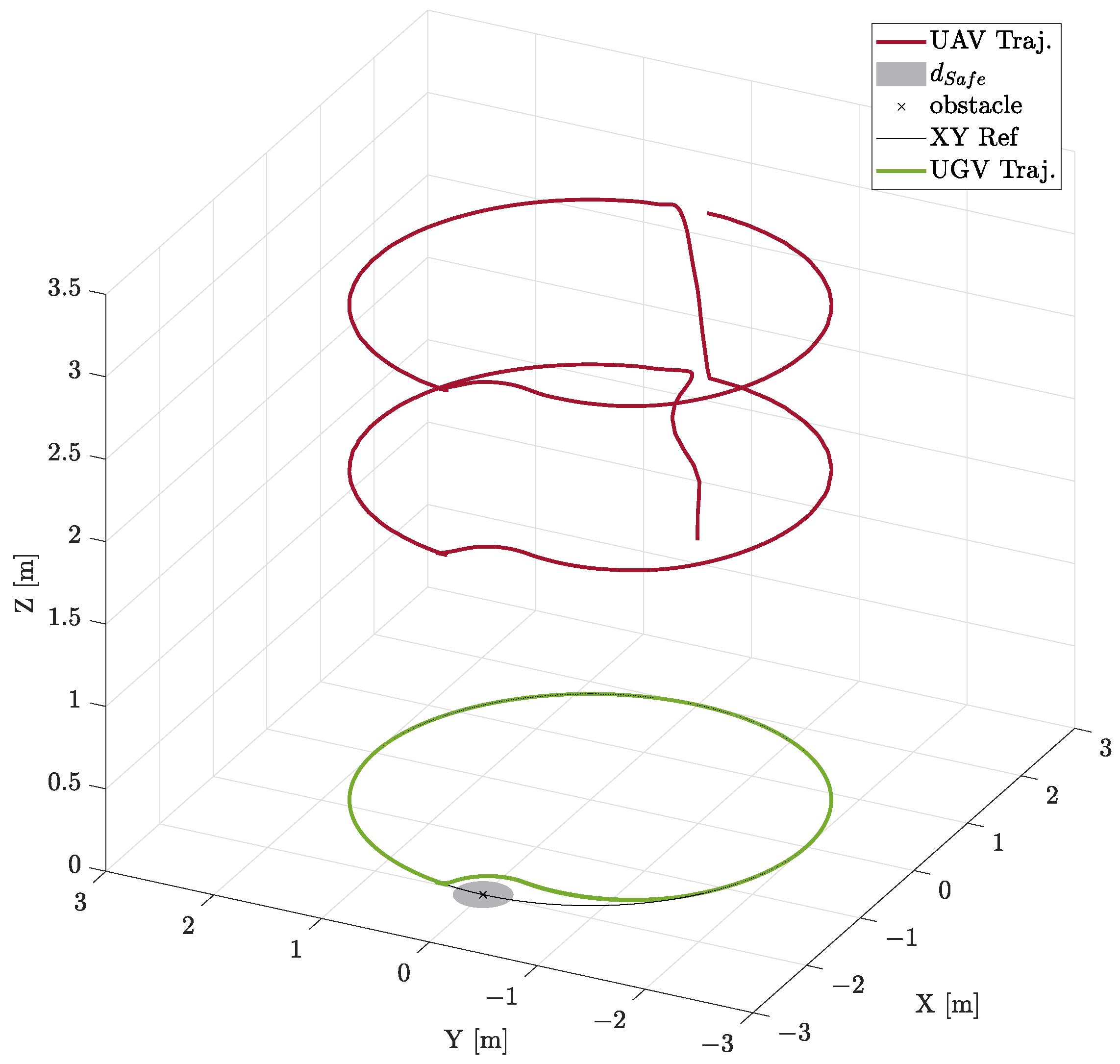
A static obstacle is placed along the reference trajectory in $(x_{Obs},y_{Obs})=(-2\mathrm{m},0\mathrm{m})$. While the UGV should track the reference, the drone should follow the leader, keeping an altitude defined as

$$z_{1,Ref}\left(t\right)=\left\{\begin{array}{c}2\mathrm{m}\mathrm{if}t<1min\hfill \\ 3\mathrm{m}\mathrm{if}t\ge 1min\hfill \end{array}\right.$$

(50)

The aim is to demonstrate that even if the drone must increase its altitude to avoid an obstacle, the controller effectively manages this change in trajectory. It should be noted that the UAV NMPC formulation currently does not include constraints such as Equation (31). Figure 4 shows the trajectories of the two agents.

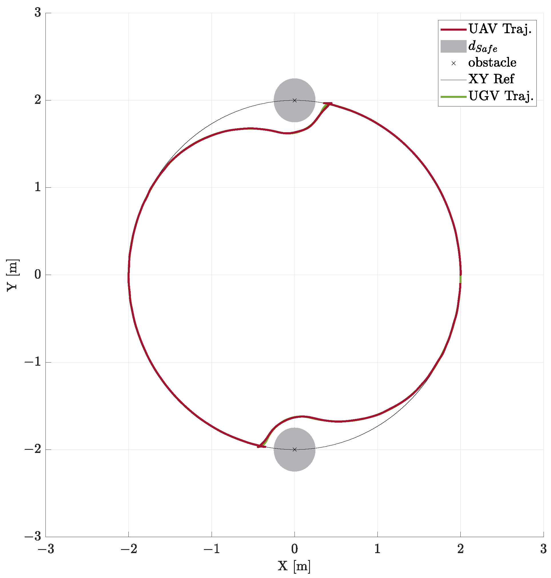
The UGV moves in a circle as long as it maintains a safe distance from the obstacle. When the car approaches the obstacle, it turns away to avoid it and then realigns with the reference trajectory as illustrated in Figure 5. Meanwhile, the UAV keeps the formation with the leader and increases its height when required.

Table 1. The UGV MHE-NMPC scheme performance—Scenario n.1.

♢	${\mathit{RMSE}}_{\mathit{x}}^{♢}$ [m]	${\mathit{RMSE}}_{\mathit{y}}^{♢}$ [m]	${\mathit{RMSE}}_{\mathit{\theta }}^{♢}$ [rad]	${\mathit{RMSE}}_{\mathit{v}}^{♢}$ [m s−1]
Equation (40)	5.30 × 10−2	1.60 × 10−1	1.53 × 10−1	5.77 × 10−2
Equation (41)	1.55 × 10−2	1.576 × 10−2	2.39 × 10−2	1.06 × 10−2
Equation (42)	3.24 × 10−5	4.46 × 10−5	6.49 × 10−4	1.73 × 10−4

summarizes all the indexes. The small errors in estimating and predicting the vehicle’s state allow to track the reference with deviations of a few centimeters and radiant.

As summed up in

Table 2. The UAV NMPC performance—Scenario n.1.

♢	${\mathit{RMSE}}_{{\mathit{x}}_1}^{♢}$ [m]	${\mathit{RMSE}}_{{\mathit{y}}_1}^{♢}$ [m]	${\mathit{RMSE}}_{{\mathit{z}}_1}^{♢}$ [m]	${\mathit{RMSE}}_{{\mathit{\psi }}_1}^{♢}$ [rad]
Equation (45)	8.30 × 10−2	8.74 × 10−2	8.94 × 10−2	6.54 × 10−2
Equation (46)	8.07 × 10−2	2.00 × 10−1	8.94 × 10−2	1.52 × 10−1

, resorting to the one-step prediction ensures the tracking of the desired attitude. Naturally, Equation (45) is smaller in magnitude than Equation (46), as in the NMPC formulation there appears ${\mathit{r}}_{UAV}\left(k\right)$ and not ${\mathit{r}}_{T,UAV}\left(k\right)$. Still, the variations from the actual reference are quite satisfactory.

Table 3. The UAV MHE performance for all components (★)—Scenario n.1.

★	${\mathit{RMSE}}_{\mathbf{★}}^{\mathit{Est},\mathit{UAV}}$	Unit
$x_1$	1.05 × 10−3	$\left[\mathrm{m}\right.]$
$x_2$	2.41 × 10−2	$\left[\mathrm{m} {\mathrm{s}}^{-1}\right.]$
$y_1$	1.01 × 10−3	$\left[\mathrm{m}\right.]$
$y_2$	2.27 × 10−2	$\left[\mathrm{m} {\mathrm{s}}^{-1}\right.]$
$z_1$	2.59 × 10−3	$\left[\mathrm{m}\right.]$
$z_2$	1.40 × 10−3	$\left[\mathrm{m} {\mathrm{s}}^{-1}\right.]$
${\theta }_1$	1.63 × 10−2	$\left[\mathrm{rad}\right.]$
${\theta }_2$	5.25 × 10−2	$\left[\mathrm{rad}{\mathrm{s}}^{-1}\right.]$
${\varphi }_1$	1.59 × 10−2	$\left[\mathrm{m}\right.]$
${\varphi }_2$	5.045 × 10−2	$\left[\mathrm{m} {\mathrm{s}}^{-1}\right.]$
${\psi }_1$	1.28 × 10−3	$\left[\mathrm{m}\right.]$
${\psi }_2$	4.18 × 10−3	$\left[\mathrm{m} {\mathrm{s}}^{-1}\right.]$

reports for each quadcopter’s state’s components the negligible estimation error.

3.2. Circle with Two Obstacles

The second case study maintains the circular trajectory previously described but considers two obstacles, placed in $(x_{Obs1},y_{Obs1})=(0\mathrm{m},2\mathrm{m})$ and $(x_{Obs2},y_{Obs2})=(0\mathrm{m},2\mathrm{m})$. The aircraft should adhere to a specified take-off reference trajectory as delineated below:

$$z_{1,Ref}\left(t\right)=\left\{\begin{array}{c}(1+(t/30\left)\right)\mathrm{m}\mathrm{if}t<30\mathrm{s}\hfill \\ 2\mathrm{m}\mathrm{if}t\ge 30\mathrm{s}\hfill \end{array}\right.$$

(51)

The simulation time is also reduced to one minute. Figure 6 and Figure 7 demonstrate that both the leader and the follower qualitatively follow the reference without collisions.

Table 4. The UGV MHE-NMPC scheme performance—Scenario n.2.

♢	${\mathit{RMSE}}_{\mathit{x}}^{♢}$ [m]	${\mathit{RMSE}}_{\mathit{y}}^{♢}$ [m]	${\mathit{RMSE}}_{\mathit{\theta }}^{♢}$ [rad]	${\mathit{RMSE}}_{\mathit{v}}^{♢}$ [m s−1]
Equation (40)	2.32 × 10−1	7.44 × 10−2	2.17 × 10−1	8.21 × 10−2
Equation (41)	1.66 × 10−2	1.61 × 10−2	3.20 × 10−2	1.50 × 10−2
Equation (42)	5.96 × 10−5	3.62 × 10−5	6.55 × 10−4	2.30 × 10−4

,

Table 5. The UAV NMPC performance—Scenario n.2.

♢	${\mathit{RMSE}}_{{\mathit{x}}_1}^{♢}$ [m]	${\mathit{RMSE}}_{{\mathit{y}}_1}^{♢}$ [m]	${\mathit{RMSE}}_{{\mathit{z}}_1}^{♢}$ [m]	${\mathit{RMSE}}_{{\mathit{\psi }}_1}^{♢}$ [rad]
Equation (45)	9.05 × 10−2	8.28 × 10−2	7.99 × 10−3	8.58 × 10−2
Equation (46)	2.80 × 10−1	9.08 × 10−2	7.99 × 10−3	2.14 × 10−1

and

Table 6. The UAV MHE performance for all components (★)—Scenario n.2.

★	${\mathit{RMSE}}_{\mathbf{★}}^{\mathit{Est},\mathit{UAV}}$	Unit
$x_1$	4.49 × 10−5	$\left[\mathrm{m}\right.]$
$x_2$	1.15 × 10−3	$\left[\mathrm{m} {\mathrm{s}}^{-1}\right.]$
$y_1$	6.87 × 10−5	$\left[\mathrm{m}\right.]$
$y_2$	1.22 × 10−3	$\left[\mathrm{m} {\mathrm{s}}^{-1}\right.]$
$z_1$	1.48 × 10−5	$\left[\mathrm{m}\right.]$
$z_2$	4.93 × 10−5	$\left[\mathrm{m} {\mathrm{s}}^{-1}\right.]$
${\theta }_1$	1.03 × 10−3	$\left[\mathrm{rad}\right.]$
${\theta }_2$	3.88 × 10−3	$\left[\mathrm{rad}{\mathrm{s}}^{-1}\right.]$
${\varphi }_1$	1.03 × 10−3	$\left[\mathrm{m}\right.]$
${\varphi }_2$	3.88 × 10−2	$\left[\mathrm{m} {\mathrm{s}}^{-1}\right.]$
${\psi }_1$	1.29 × 10−3	$\left[\mathrm{m}\right.]$
${\psi }_2$	4.19 × 10−3	$\left[\mathrm{m} {\mathrm{s}}^{-1}\right.]$

show the performance indices for both agents. In order to avoid the two obstacles, the ground robot has to deviate its trajectory, which leads to an increase in its $RMS{E}_x^{◊}$ of Equation (40). The drone accurately follows the one-step prediction of the car. However, the increase in the leader’s tracking error caused by the obstacles is reflected in the follower’s performance.

3.3. Lemniscate of Bernoulli with One Obstacle

For the third simulation, Bernoulli’s lemniscate is chosen as the desired trajectory, described by the following equations:

$$\left\{\begin{array}{cc}{x}_{Ref}\left(t\right)\hfill & =2c\left(t\right)cos\left(t{\displaystyle \frac{2\pi }{60}}\right)\hfill \\ y_{Ref}\left(t\right)\hfill & =c\left(t\right)sin\left(2t{\displaystyle \frac{2\pi }{60}}\right)\hfill \\ {\theta }_{Ref}\left(t\right)\hfill & =\arctan 2(v_{y,Ref}\left(t\right),v_{x,Ref}\left(t\right))\hfill \\ v_{Ref}\left(t\right)\hfill & =\sqrt{v_{x,Ref}{\left(t\right)}^2+v_{y,Ref}{\left(t\right)}^2}\hfill \end{array}\right.$$

(52)

with

$$c\left(t\right)=2/\left(3-cos\left(2t{\displaystyle \frac{2\pi }{60}}\right)\right)$$

(53)

$$v_{x,Ref}\left(t\right)={\left.{\displaystyle \frac{d{x}_{Ref}\left(\tau \right)}{d\tau }}\right|}_{\tau =t}{v}_{y,Ref}\left(t\right)={\left.{\displaystyle \frac{d{y}_{Ref}\left(\tau \right)}{d\tau }}\right|}_{\tau =t}$$

(54)

and the only obstacle is in the origin. The reference altitude of the UAV is kept constant at $z_{1,Ref}\left(t\right)=2\mathrm{m}$.

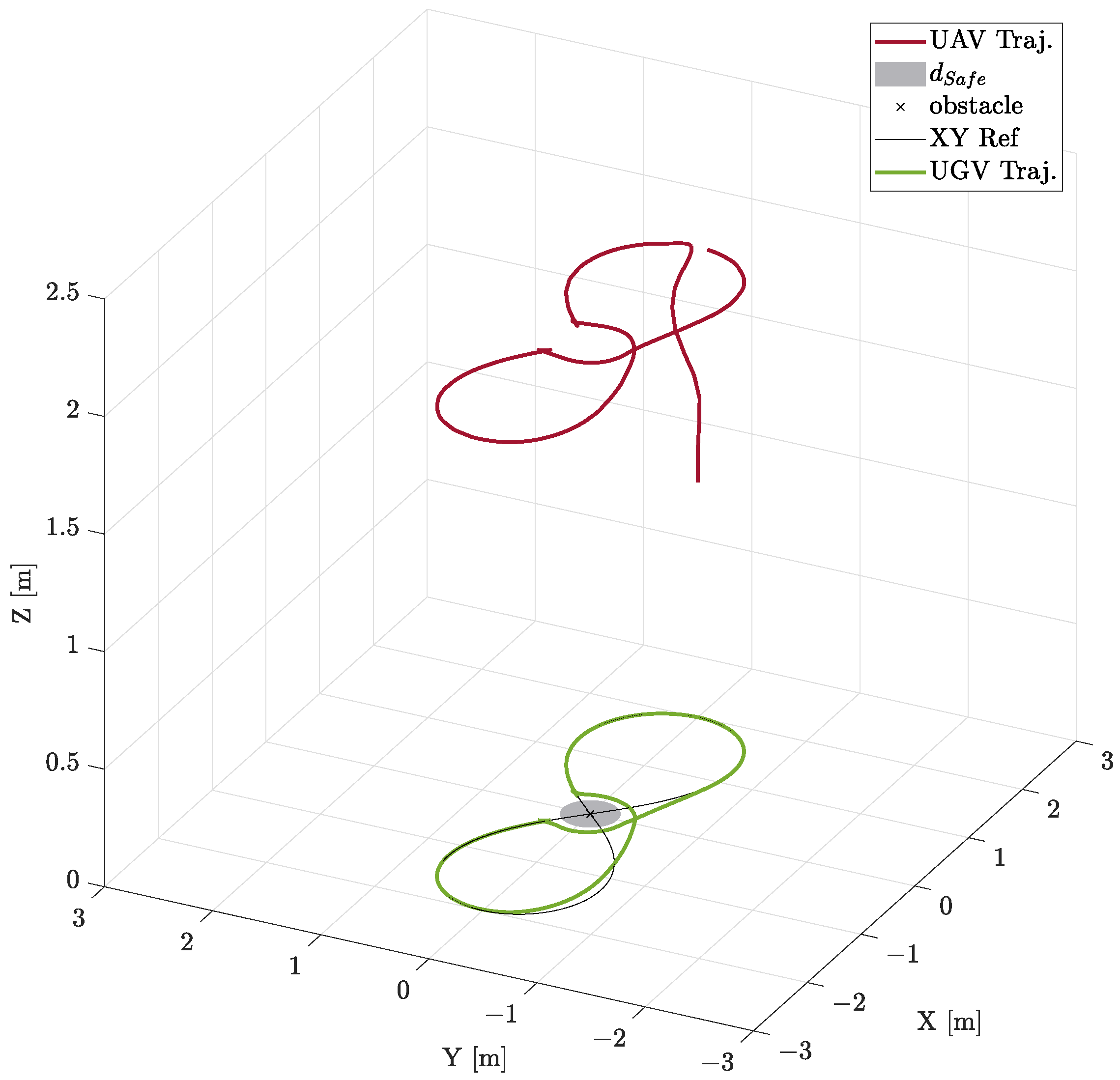
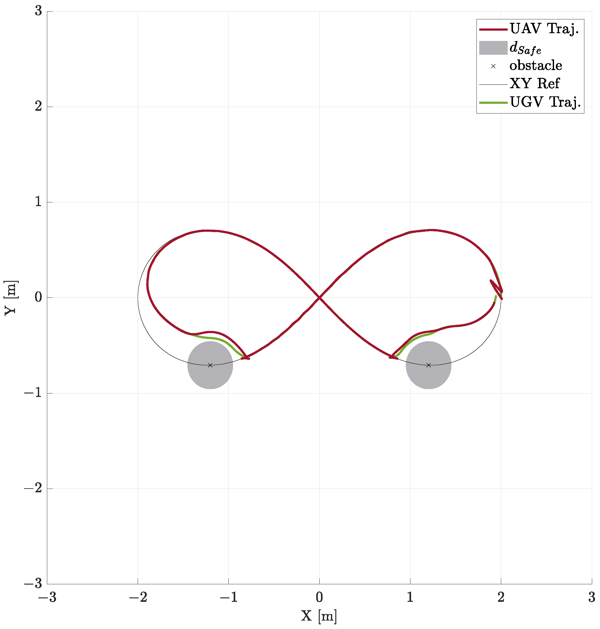
The trajectories of the two agents are depicted in Figure 8 and Figure 9. The UGV initially follows the lemniscate path until it approaches too close to the origin. At that point, it navigates around the obstacle, resulting in a decrease in tracking accuracy as shown in

Table 7. The UGV MHE-NMPC scheme performance—Scenario n.3.

♢	${\mathit{RMSE}}_{\mathit{x}}^{♢}$ [m]	${\mathit{RMSE}}_{\mathit{y}}^{♢}$ [m]	${\mathit{RMSE}}_{\mathit{\theta }}^{♢}$ [rad]	${\mathit{RMSE}}_{\mathit{v}}^{♢}$ [m s−1]
Equation (40)	3.26 × 10−1	1.93 × 10−1	2.84 × 10−1	9.55 × 10−2
Equation (41)	1.79 × 10−2	1.62 × 10−2	3.39 × 10−2	1.53 × 10−2
Equation (42)	1.17 × 10−4	6.36 × 10−5	7.02 × 10−4	5.13 × 10−4

. Due to the control constraints, the agent gradually returns to the reference path without sudden movements. When the steering car returns to its starting point, it must pass the origin again, thereby repeating the same behavior. Regarding the quadcopter, except for the initial moments of the simulation due to the initial conditions, it maintains the desired height while following the leader from above. For a quantitative analysis, see

Table 8. The UAV NMPC performance—Scenario n.3.

♢	${\mathit{RMSE}}_{{\mathit{x}}_1}^{♢}$ [m]	${\mathit{RMSE}}_{{\mathit{y}}_1}^{♢}$ [m]	${\mathit{RMSE}}_{{\mathit{z}}_1}^{♢}$ [m]	${\mathit{RMSE}}_{{\mathit{\psi }}_1}^{♢}$ [rad]
Equation (45)	9.16 × 10−2	7.01 × 10−2	8.46 × 10−2	9.53 × 10−2
Equation (46)	3.63 × 10−1	2.16 × 10−1	8.46 × 10−2	2.90 × 10−1

and

Table 9. The UAV MHE performances for all components (★)—Scenario n.3.

★	${\mathit{RMSE}}_{\mathbf{★}}^{\mathit{Est},\mathit{UAV}}$	Unit
$x_1$	8.14 × 10−4	$\left[\mathrm{m}\right.]$
$x_2$	1.84 × 10−2	$\left[\mathrm{m} {\mathrm{s}}^{-1}\right.]$
$y_1$	1.25 × 10−3	$\left[\mathrm{m}\right.]$
$y_2$	2.82 × 10−2	$\left[\mathrm{m} {\mathrm{s}}^{-1}\right.]$
$z_1$	2.57 × 10−3	$\left[\mathrm{m}\right.]$
$z_2$	1.13 × 10−3	$\left[\mathrm{m} {\mathrm{s}}^{-1}\right.]$
${\theta }_1$	1.23 × 10−2	$\left[\mathrm{rad}\right.]$
${\theta }_2$	3.92 × 10−2	$\left[\mathrm{rad}{\mathrm{s}}^{-1}\right.]$
${\varphi }_1$	1.97 × 10−2	$\left[\mathrm{m}\right.]$
${\varphi }_2$	6.21 × 10−2	$\left[\mathrm{m} {\mathrm{s}}^{-1}\right.]$
${\psi }_1$	1.29 × 10−3	$\left[\mathrm{m}\right.]$
${\psi }_2$	4.21 × 10−3	$\left[\mathrm{m} {\mathrm{s}}^{-1}\right.]$

.

3.4. Lemniscate of Bernoulli with Two Obstacles

The last case study is similar to the previous one, but a second obstacle is added. Both are in the reference positions that the robot should ideally pass at $t=24\mathrm{s}$ and $t=54\mathrm{s}$. To complicate the test, the constant height is replaced by a decreasing trajectory:

$$z_{1,Ref}\left(t\right)=\left\{\begin{array}{c}2\mathrm{m}\mathrm{if}t<30\mathrm{s}\hfill \\ 2-\left(1.8\right(t-30)/30)\mathrm{m}\mathrm{if}t\ge 30\mathrm{s}\hfill \end{array}\right.$$

(55)

The resulting performance indices are presented in

Table 10. The UGV MHE-NMPC scheme performance—Scenario n.4.

♢	${\mathit{RMSE}}_{\mathit{x}}^{♢}$ [m]	${\mathit{RMSE}}_{\mathit{y}}^{♢}$ [m]	${\mathit{RMSE}}_{\mathit{\theta }}^{♢}$ [rad]	${\mathit{RMSE}}_{\mathit{v}}^{♢}$ [m s−1]
Equation (40)	2.17 × 10−1	4.61 × 10−2	2.03 × 10−1	7.65 × 10−2
Equation (41)	1.50 × 10−2	1.92 × 10−2	3.46 × 10−2	1.51 × 10−2
Equation (42)	2.91 × 10−5	2.85 × 10−5	6.94 × 10−4	9.77 × 10−5

,

Table 11. The UAV NMPC performance—Scenario n.4.

♢	${\mathit{RMSE}}_{{\mathit{x}}_1}^{♢}$ [m]	${\mathit{RMSE}}_{{\mathit{y}}_1}^{♢}$ [m]	${\mathit{RMSE}}_{{\mathit{z}}_1}^{♢}$ [m]	${\mathit{RMSE}}_{{\mathit{\psi }}_1}^{♢}$ [rad]
Equation (45)	8.22 × 10−2	6.10 × 10−2	1.12 × 10−1	9.20 × 10−2
Equation (46)	2.54 × 10−1	6.30 × 10−2	1.13 × 10−1	2.18 × 10−1

and

Table 12. The UAV MHE performance for all components (★)—Scenario n.4.

★	${\mathit{RMSE}}_{\mathbf{★}}^{\mathit{Est},\mathit{UAV}}$	Unit
$x_1$	8.14 × 10−4	$\left[\mathrm{m}\right.]$
$x_2$	1.84 × 10−2	$\left[\mathrm{m} {\mathrm{s}}^{-1}\right.]$
$y_1$	1.25 × 10−3	$\left[\mathrm{m}\right.]$
$y_2$	2.82 × 10−2	$\left[\mathrm{m} {\mathrm{s}}^{-1}\right.]$
$z_1$	2.57 × 10−3	$\left[\mathrm{m}\right.]$
$z_2$	1.13 × 10−3	$\left[\mathrm{m} {\mathrm{s}}^{-1}\right.]$
${\theta }_1$	1.22 × 10−2	$\left[\mathrm{rad}\right.]$
${\theta }_2$	3.92 × 10−2	$\left[\mathrm{rad}{\mathrm{s}}^{-1}\right.]$
${\varphi }_1$	1.97 × 10−2	$\left[\mathrm{m}\right.]$
${\varphi }_2$	6.21 × 10−2	$\left[\mathrm{m} {\mathrm{s}}^{-1}\right.]$
${\psi }_1$	1.29 × 10−3	$\left[\mathrm{m}\right.]$
${\psi }_2$	4.21 × 10−3	$\left[\mathrm{m} {\mathrm{s}}^{-1}\right.]$

. As can be seen from Figure 10 and Figure 11, considerations similar to those for the single barrier case can be drawn. Note that the RSME_x and RMSE_y of the tracking error Equation (40) are smaller compared to the values in the first row of Table 10, which remain the worst values among all the simulations. Nevertheless, in none of the case studies did the errors diverge and the ground vehicle entered the unsafe region.

4. Discussion

In this paper, nonlinear rolling horizon techniques are applied to a heterogeneous fleet. In particular, a distributed solution is proposed to address the formation path-tracking problem while avoiding obstacles. Results across various scenarios and maneuvers confirm the validity of the proposed control architecture, ensuring small errors with respect to reference trajectories. The possibilities for future research are manifold. Firstly, the results suggest that the proposed scheme ensures small tracking errors, but still the stability and convergence of the NMPC should be proved in a more rigorous way. Secondly, the works [5,6,7,8] indicate the superiority of NMPC over classical controllers. Conducting a similar comparative analysis, particularly in scenarios involving data loss, would be valuable to quantify the improvements in performance brought by the usage of a NMPC. Lastly, to go beyond numerical simulation, the implementation and embedding of the control architecture in real robots, such as the Parrot Bebop 2.0 and JetRacer equipped with LIDAR mapping, would strengthen the validation and applicability of the proposed methods in practical scenarios.

References

1. Verma, J.K.; Ranga, V. Multi-Robot Coordination Analysis, Taxonomy, Challenges and Future Scope. J. Intell. Robot. Syst. 2021, 102, 10. [Google Scholar] [CrossRef] [PubMed]
2. Bacheti, V.P.; Brandão, A.S.; Sarcinelli-Filho, M. A Path-Following Controller for a UAV-UGV Formation Performing the Final Step of Last-Mile-Delivery. IEEE Access 2021, 9, 142218–142231. [Google Scholar] [CrossRef]
3. Zhang, J.; Yue, X.; Zhang, H.; Xiao, T. Optimal Unmanned Ground Vehicle—Unmanned Aerial Vehicle Formation-Maintenance Control for Air-Ground Cooperation. Appl. Sci. 2022, 12, 3598. [Google Scholar] [CrossRef]
4. Tassanbi, A.; Iskakov, A.; Do, T.D.; Ali, M.H. Interactive Real-time Leader Follower Control System for UAV and UGV. In Proceedings of the 2022 International Conference on Electrical, Computer, Communications and Mechatronics Engineering (ICECCME), Male, Malediven, 16–18 November 2022; pp. 1–8. [Google Scholar] [CrossRef]
5. Okasha, M.; Kralev, J.K.; Islam, M. Design and Experimental Comparison of PID, LQR and MPC Stabilizing Controllers for Parrot Mambo Mini-Drone. Aerospace 2022, 9, 298. [Google Scholar] [CrossRef]
6. Al-Saoudi, A.F.; Al-Aubidy, K.M.; Al-Mahasneh, A.J. Comparison of PID, Fuzzy Logic, ANFIS and Model Predictive Controllers for Cruise Control System. In Proceedings of the 2024 21st International Multi-Conference on Systems, Signals & Devices (SSD), Erbil, Iraq, 22–25 April 2024; pp. 263–265. [Google Scholar]
7. Kaçmaz, B.; Söylemez, M.T. Implementation and Comparison of PID, PI-PD, LQR and MPC on Separation Clutch System in Slip. In Proceedings of the 2021 22nd IEEE International Conference on Industrial Technology (ICIT), Valencia, Spain, 10–12 March 2021; Volume 1, pp. 61–67. [Google Scholar]
8. Liu, J.; Yang, Z.; Huang, Z.; Li, W.; Dang, S.; Li, H. Simulation Performance Evaluation of Pure Pursuit, Stanley, LQR, MPC Controller for Autonomous Vehicles. In Proceedings of the 2021 IEEE International Conference on Real-Time Computing and Robotics (RCAR), Xining, China, 15–19 July 2021; pp. 1444–1449. [Google Scholar]
9. Cenerini, J.; Mehrez, M.W.; Han, J.w.; Jeon, S.; Melek, W. Model Predictive Path Following Control without terminal constraints for holonomic mobile robots. Control Eng. Pract. 2023, 132, 105406. [Google Scholar] [CrossRef]
10. Bozzi, A.; Graffione, S.; Kockelkoren, M.M.; Sacile, R.; Zero, E. Path Tracking for Wheeled Mobile Robot Using Non Linear Model Predictive Control in Indoor Environment. In Proceedings of the 2023 9th International Conference on Control, Decision and Information Technologies (CoDIT), Rome, Italy, 3–6 July 2023; pp. 1379–1384. [Google Scholar] [CrossRef]
11. Recalde, L.F.; Guevara, B.S.; Andaluz, V.; Varela, J.; Gimenez, J.; Gandolfo, D. Nonlinear MPC for Multiple Quadrotors in Dynamic Environments. In Proceedings of the 2022 International Conference on Unmanned Aircraft Systems (ICUAS), Dubrovnik, Croatia, 21–24 June 2022; pp. 1201–1209. [Google Scholar] [CrossRef]
12. Biegler, L. A perspective on nonlinear model predictive control. Korean J. Chem. Eng. 2021, 38, 1317–1332. [Google Scholar] [CrossRef]
13. Deniz, N.; Jorquera, F.; Torres-Torriti, M.; Cheein, F.A. Model predictive path-following controller for Generalised N-Trailer vehicles with noisy sensors and disturbances. Control Eng. Pract. 2024, 142, 105747. [Google Scholar] [CrossRef]
14. Aaltonen, O. Nonlinear Model Predictive Control and Estimation applied to Selective Catalytic Reduction. Master’s Thesis, Åbo Akademi University, Turku, Finland, 2022. [Google Scholar]
15. Lindqvist, B.; Mansouri, S.S.; Agha-mohammadi, A.A.; Nikolakopoulos, G. Nonlinear MPC for collision avoidance and control of UAVs with dynamic obstacles. IEEE Robot. Autom. Lett. 2020, 5, 6001–6008. [Google Scholar] [CrossRef]
16. Eltrabyly, A.; Ichalal, D.; Mammar, S. Quadcopter Trajectory Tracking in the Presence of 4 Faulty Actuators: A Nonlinear MHE and MPC Approach. IEEE Control Syst. Lett. 2022, 6, 2024–2029. [Google Scholar] [CrossRef]
17. Castillo Garcia, P.; Munoz, L.; Gil, P. Modeling Approaches—The results in this chapter were developed in collaboration with H. Abaunza and J. Carino from the UMI LAFMIA 3175, Mexico. In Indoor Navigation Strategies for Aerial Autonomous Systems; Elsevier: Amsterdam, The Netherlands, 2017; pp. 31–50. [Google Scholar] [CrossRef]
18. Lin, X.; Chen, X. Realization of Ackermann robot obstacle avoidance navigation based on Multi-sensor fusion SLAM. In Proceedings of the 2023 5th International Conference on Electronics and Communication, Network and Computer Technology (ECNCT), Guangzhou, China, 18–20 August 2023; pp. 354–359. [Google Scholar] [CrossRef]
19. Köhler, J.; Müller, M.A.; Allgöwer, F. A nonlinear tracking model predictive control scheme for dynamic target signals. Automatica 2020, 118, 109030. [Google Scholar] [CrossRef]
20. Sani, M.; Robu, B.; Hably, A. Dynamic Obstacles Avoidance Using Nonlinear Model Predictive Control. In Proceedings of the IECON 2021—47th Annual Conference of the IEEE Industrial Electronics Society, Toronto, ON, Canada, 13–16 October 2021; pp. 1–6. [Google Scholar] [CrossRef]
21. Andersson, J.A.E.; Gillis, J.; Horn, G.; Rawlings, J.B.; Diehl, M. CasADi—A software framework for nonlinear optimization and optimal control. Math. Program. Comput. 2019, 11, 1–36. [Google Scholar] [CrossRef]
Figure 1. The quadcopter state consists of its position, translational velocity (both in the global reference frame), orientation, and rotational velocities (expressed in terms of Euler angles and in the body frame). The dynamics are obtained using the Euler–Lagrange approach.
Automation 05 00020 g001
Figure 2. UGV Ackermann’s dynamic model with corresponding state and control variables.
Automation 05 00020 g002
Figure 3. Obstacles are detected up to a distance d L I D A R , and the UGV should keep a safe distance d S a f e .
Automation 05 00020 g003
Figure 4. Trajectories of the two robots versus the reference. In grey, the unsafe obstacle’s neighborhood.
Automation 05 00020 g004
Figure 5. Top view of the trajectory of the UVs. Although the reference passes close to the obstacle, the steering car deviates to keep the safe distance.
Automation 05 00020 g005
Figure 6. Trajectories of the two robots versus the reference. The drone increases, in the first half of the simulation, its altitude up to 2 m .
Automation 05 00020 g006
Figure 7. Top view of the trajectory of the UVs in the second scenario with two obstacles along the reference trajectory.
Automation 05 00020 g007
Figure 8. Trajectories of the two robots versus the reference. The drone’s reference altitude is 2 m.
Automation 05 00020 g008
Figure 9. Top view of the trajectory of the UVs in the third scenario with the reference trajectory of the lemniscate of Bernoulli.
Automation 05 00020 g009
Figure 10. Trajectories of the ground and the aerial robots. The UGV has to follow the lemniscate of Bernoulli trajectory while avoiding two obstacles on its way. The quadcopter in the second half of the simulation reduces its height.
Automation 05 00020 g010
Figure 11. Top view of the two agents’ paths compared with the reference in the fourth scenario.
Automation 05 00020 g011