Article

Enhancing Quadcopter Autonomy: Implementing Advanced Control Strategies and Intelligent Trajectory Planning

by
Samira Hadid
1,*,
Razika Boushaki
2,
Fatiha Boumchedda
3 and
Sabrina Merad
3
1
Laboratoire Ingénierie des Systèmes et Télécommunications, Faculté de Technologie, Université M’hamed BOUGARA de Boumerdes (UMBB), Boumerdes 35000, Algeria
2
Laboratoire d’Automatique Appliquée, Institut de Génie Electrique et Electronique, Université M’hamed BOUGARA de Boumerdes (UMBB), Boumerdes 35000, Algeria
3
Institut de Génie Electrique et Electronique, Université M’hamed BOUGARA de Boumerdes, Boumerdes 35000, Algeria
*
Author to whom correspondence should be addressed.
Automation 2024, 5(2), 151-175; https://doi.org/10.3390/automation5020010
Submission received: 13 May 2024 / Revised: 8 June 2024 / Accepted: 11 June 2024 / Published: 14 June 2024

Abstract

:
In this work, an in-depth investigation into enhancing quadcopter autonomy and control capabilities is presented. The focus lies on the development and implementation of three conventional control strategies to regulate the behavior of quadcopter UAVs: a proportional–integral–derivative (PID) controller, a sliding mode controller, and a fractional-order PID (FOPID) controller. Utilizing careful adjustments and fine-tuning, each control strategy is customized to attain the desired dynamic response and stability during quadcopter flight. Additionally, an approach called Dyna-Q learning for obstacle avoidance is introduced and seamlessly integrated into the control system. Leveraging MATLAB as a powerful tool, the quadcopter is empowered to autonomously navigate complex environments, adeptly avoiding obstacles through real-time learning and decision-making processes. Extensive simulation experiments and evaluations, conducted in MATLAB 2018a, precisely compare the performance of the different control strategies, including the Dyna-Q learning-based obstacle avoidance technique. This comprehensive analysis allows us to understand the strengths and limitations of each approach, guiding the selection of the most effective control strategy for specific application scenarios. Overall, this research presents valuable insights and solutions for optimizing flight stability and enabling secure and efficient operations in diverse real-world scenarios.

1. Introduction

As technology continues to evolve, the domain of drones presents a fascinating landscape of innovation. Among the diverse types of drones available, quadcopters stand out as highly promising and versatile unmanned aerial vehicles (UAVs), known for their exceptional maneuverability and ability to navigate challenging terrain. They have become invaluable tools in diverse applications, such as surveillance and disaster response [1,2]. To fully harness their capabilities, it is essential to develop advanced control strategies and trajectory planning techniques that can effectively adapt to dynamic environments and avoid obstacles [3,4,5,6,7].
For implementation and simulation, various linear, nonlinear, and robust controllers have been studied [8,9,10]. The PID and FOPID controllers have been applied on height, x and y positions, and roll, pitch, and yaw angles. Li, J. et al. proposed a trajectory-tracking control of a quadrotor based on a fractional-order S-Plane model; their study focused on the low tracking accuracy and weak anti-interference ability of quadcopter drones in trajectory-tracking control [11]. Ademola, A. et al.’s study investigated the problem of the nonlinear quadcopter system’s mathematical modeling and control for stabilization and trajectory tracking using the feedback linearization (FBL) technique combined with the PD controller [12]. The implementation of a robust sliding mode controller (SMC) for trajectory tracking has been carried out by Yih, C.-C. et al. They demonstrate from the Lyapunov stability theorem that the proposed control scheme can guarantee the asymptotic stability of the tilt-rotor quadcopter in terms of position and attitude following control allocation [13]. The Dyna-Q learning-based obstacle avoidance technique was the subject of many research works and was applied to a wide range of quadcopter controllers [14,15,16]. Budiyanto, A. et al. proposed the application of the Deep Dyna-Q algorithm in formation control in both simulations and actual experiments [15].
The main objectives of this work revolve around enhancing quadcopter autonomy and control capabilities through comprehensive investigation. The first section of this work explores the principles of flight dynamics, encompassing the mechanics that govern quadcopter movement. The second section delves into the modeling aspect, presenting a detailed mathematical representation of quadcopter dynamics. This comprehensive quadcopter model covers both kinematics and dynamics, serving as a robust framework for controller design and stability analysis. Utilizing this model, we proceed to implement three distinct control approaches: the proportional–integral–derivative (PID) controller, the fractional-order PID controller, and the sliding mode controller (SMC).
The PID controller, widely known for its simplicity and widespread use, serves as the baseline for comparison among the control strategies. Additionally, the project explores the integration of fractional calculus into the PID controller to enhance control performance, particularly in managing system nonlinearities and uncertainties [6]. Furthermore, the sliding mode controller’s robustness against disturbances was evaluated.
In the final section of this work, the crucial aspect of obstacle avoidance is addressed through the development of an intelligent trajectory planning approach using Dyna-Q learning. This approach leverages real-time environmental data to generate safe and efficient paths for quadcopters, enabling them to autonomously navigate complex environments while intelligently avoiding obstacles. The proposed control strategies, together with trajectory planning using Dyna-Q learning, undergo extensive validation through simulations employing various performance metrics.
The anticipated outcomes of this research include significant advancements in quadcopter autonomy, enabling their deployment in increasingly challenging scenarios. By integrating advanced control strategies and intelligent trajectory planning, we aim to enhance the quadcopter’s adaptability and responsiveness, making them indispensable assets in applications such as search and rescue missions, precision agriculture, and infrastructure inspection. Through an in-depth understanding of the strengths and limitations of various control strategies and innovative approaches like Dyna-Q learning, we strive to unlock the full potential of quadcopters and pave the way for their widespread adoption in diverse applications.

2. Quadcopter State Space Model

The state space vector X describes the position of the quadcopter in space and its linear and angular velocities as follows [5,6,7,8,17,18,19,20]:
X = x x ˙ y y ˙ z z ˙         ϕ ϕ ˙ θ θ ˙ ψ ψ ˙ T
The control input vector for a quadcopter state space model is represented as follows:
U = [U1 U2 U3 U4] T
where U1 controls the quadcopter’s total thrust that is responsible for quadcopter altitude, while U2, U3, and U4 control the moments that result in roll, pitch, and yaw angles, respectively, enabling precise control and stabilization of the quadcopter in response to external disturbances.
Figure 1 illustrates the movement of a quadcopter in space. The x, y, and z variables represent the displacements of the quadcopter’s center of mass from an Earth-fixed inertial frame along the respective x, y, and z axes. The quadcopter’s orientation is represented by the three Euler angles: φ represents the roll angle around the x-axis, θ represents the pitch angle around the y-axis, and ψ represents the yaw angle around the z-axis [5,6,7].
In order to obtain the state space representation of the quadcopter, the following equations that describe the translational and rotational motion of the quadcopter are used [17,18,19,20]:
x ¨ = U 1 m t ( sin ϕ sin ψ + cos ϕ sinθ c o s ψ ) A x x ˙ m t y ¨ = U 1 m t cos ϕ s i n θ s i n ψ s i n ϕ c o s ψ A y y ˙ m t z ¨ = U 1 m t cos ϕ c o s θ g A z z ˙ m t
The translation equation of motion in terms of control input is shown above;
ϕ ¨ = θ ˙ ϕ ˙ a 1 + b 1 l U 2 θ ˙ a 2 ω r z K a x b 1 ϕ ˙ θ ¨ = ϕ ˙ ψ ˙ a 3 + b 2 l U 3 ϕ ˙ a 4 ω r z K a y b 2 θ ˙ ψ ¨ = b 3 U 4 K a z b 3 ψ ˙
And the rotational equation of motion in terms of control input is shown above,
where:
  • mt is the total mass of the quadcopter;
  • K a x and K a y     ,   K a z   a r e the aerodynamics rotation coefficients matrix;
  • ω r z is the rotor’s angular velocities about the axis where the rotation occurs (z-axis).
And
a 1 = I y y I z z I x x ,   a 2 = I r I x x ,   a 3 = I z z I x x I y y ,   a 4 = I r I y y ,   b 1 = 1 I x x ,   b 2 = 1 I y y ,   b 3 = 1 I z z
I x x , I y y , and I z z are the mass moments of inertia about the three principal axes in the body frame.
The nonlinear state differential equations are expressed according to the following:
x 1 ˙ = x 2   x 2 ˙ = U 1 m t ( sin x 7 sin x 11 + cos x 7 sin x 9 c o s x 11 ) A x x 2 m t x 3 ˙ = x 4 x 4 ˙ = U 1 m t cos x 7 s i n x 9 s i n x 11 s i n x 7 c o s x 11 A y x 4 m t x 5 ˙ = x 6 x 6 ˙ = U 1 m t cos x 7 c o s x 9 g A z x 6 m t x 7 ˙ = x 8 x 8 ˙ = x 10 x 8 a 1 + b 1 l U 2 x 10 a 2 ω r z K a x b 1 x 8 x 9 ˙ = x 10 x 10 ˙ = x 8 x 12 a 3 + b 2 l U 3 x 8 a 4 ω r z K a y   b 2 x 10 x 11 ˙ = x 12 x 12 ˙ = b 3 U 4 K a z   b 3 x 12

3. Quadcopter Control Methods

3.1. PID Controller

PID controllers, known as proportional–integral–derivative controllers, are widely employed due to their simplicity and high efficiency in numerous industrial applications [19,20,21,22]. To design the PID controller for the nonlinear system, an initial step involves designing and tuning a controller for the linearized model. Subsequently, the designed controller is then implemented on the nonlinear quadcopter system. This approach simplifies the control design process by utilizing classical control techniques suitable for linear systems, allowing for an effective starting point in achieving stabilization. However, it is crucial to acknowledge that the linearized model is an approximation and may not fully capture all the complexities of the quadcopter’s nonlinear dynamics. Therefore, further adjustments and fine-tuning of the actual nonlinear system may be required to optimize stability and overall performance in varying operating conditions.
Altitude Controller: A PID controller is designed to control the quadcopter’s altitude, generating the control input U1 that governs the quadcopter’s altitude as shown below:
U 1 = K P e z + K i e z + K D d e z d t + g m t
Roll Controller: A PID controller is designed to generate the control input U2 that governs the quadcopter’s roll motion. The control law is presented by the following:
U 2 = K P e ϕ + K i e ϕ + K D d e ϕ d t
Pitch Controller: a PID controller is designed to generate the control input U3 that governs the quadcopter’s pitch motion. The control law is presented by the following:
U 3 = K P e θ + K i e θ + K D d e θ d t
Heading Control: A PID controller is designed to generate the control input U4 that governs the quadcopter’s yaw motion. The control law is presented by the following:
U 4 = K P e ψ + K i e ψ + K D d e ψ d t
Position Control: To control the position, two PID controllers are designed to generate the control signals, Ux and Uy, which represent the accelerations, x ¨ and y ¨ , respectively. The formulated control laws are presented by the following:
U x = x ¨ = K P e x + K i e x + K D d e x d t U y = y ¨ = K P e y + K i e y + K D d e y d t

3.2. Fractional-Order Controller

The nonlinear fractional controller, known as the P I λ D μ controller, represents a broader form of the classical PID controller. It expands the conventional integral and differential orders, λ and μ, beyond integer values into the real and complex domains [11,23,24]. Table 1 resumes all possible configurations for the types of classical PID controllers, which are determined by the values of μ and λ:
The transfer function of a fractional-order controller has the following form:
U s = E s K P + K I s λ + K D s μ
The equation for the P I λ D μ controller output in the time domain is as follows:
u t = K P e t + K I D λ e ( t ) + K D D μ e ( t )
K P , K I ,   a n d   K D represent the proportional, integral, and derivative gains, respectively, and e ( t ) denotes the error between the desired and the obtained results. In addition to these parameters, the FOPID controller introduces two additional degrees of freedom, μ and λ, which play a crucial role in enhancing the controller’s performance and providing greater flexibility in its design. These extra degrees of freedom allow for superior control capabilities and improved adaptability to various control tasks. After obtaining the appropriate PID gains for the nonlinear system, we proceeded to implement these gains into the fractional-order PID (FOPID) controller. The FOPID controller is designed using the FOMCON toolbox in MATLAB 2018a, which allows for tuning the parameters μ and λ for each controller. Through a systematic process, we fine-tuned these parameters and made necessary adjustments to the gains to account for any observed system oscillations. This iterative tuning procedure aimed to achieve improved control performance and stability for the quadcopter system under consideration.

3.3. Sliding Mode Controller

The sliding mode controller (SMC) technique is a nonlinear control approach that alters the dynamics of a nonlinear system using a discontinuous control signal. This signal compels the system to slide along a predefined cross-section of its normal behavior, showcasing remarkable accuracy and robustness [12,25,26]. The SMC technique comprises two essential components. Firstly, a discontinuous control law is employed to drive the error vector towards a specific decision rule, referred to as the sliding surface. Once the error vector reaches this surface, a continuous component of the controller takes over to follow the system dynamics defined by the equations characterizing the sliding surface. The selection of the sliding surface or decision rule is a critical aspect and is based on performance criteria since it determines the system’s dynamics. Therefore, it can be expressed as follows [12]:
s = e ˙ + λ e
where S is the sliding surface, λ is a positive tuning parameter, and e is the tracking error;
s ˙ = K 1 s i g n s K 2 s
and where K1, K2 are positive tuning parameters.
The sliding surface, its derivative, develops controllers for attitude, altitude, position, and heading.
Altitude sliding mode controller:
Considering the error between the desired altitude and the actual one provides the following equation:
e z = z d z
The error in Equation (13) is replaced in Equations (14) and (15), and thus the following equations are obtained:
s z = ( z d ˙ z ˙ ) + λ   ( z d z ) s z ˙ = z d ¨ z ¨ + λ ( z d ˙ z ˙ ) s z ˙ = k 1 s i g n s z k 2 ( s z )
Equation (16) can be written as follows:
z d ¨ z ¨ + λ ( z d ˙ z ˙ ) = k 1 s i g n s z k 2 ( s z )
The control input U1 law is obtained and represented by the following equation:
U 1 = m ( z d ¨ + g + A z z ˙ m + λ z d ˙ z ˙ + k 1 s i g n s z + k 2 ( s z ) ) cos ϕ c o s θ  
The attitude sliding mode controllers are presented below:
Roll controller:
ϕ d ¨ ϕ ¨ + λ ( ϕ d ˙ ϕ ˙ ) = k 1 s i g n s ϕ k 2 ( s ϕ )
The control input U2 law is obtained and represented by the following equation:
U 2 = ϕ d ¨ θ ˙ ϕ ˙ a 1 + θ ˙ a 2 ω r z + K a x b 1 ϕ ˙ + λ ϕ d ˙ ϕ ˙ + k 1 s i g n s ϕ + k 2 ( s ϕ ) b 1 l
Pitch controller:
θ d ¨ θ ¨ + λ ( θ d ˙ θ ˙ ) = k 1 s i g n s θ k 2 ( s θ )
The control input U3 law is obtained and represented by the following equation:
U 3 = θ d ¨ ϕ ˙ ψ ˙ a 3 + ϕ ˙ a 4 ω r z + K a y b 2 θ ˙ + λ θ d ˙ θ ˙ + k 1 s i g n s θ + k 2 ( s θ ) b 2 l
Heading sliding mode controller:
ψ d ¨ ψ ¨ + λ ( ψ d ˙ ψ ˙ ) = k 1 s i g n s ψ k 2 ( s ψ )
The control input law is obtained and represented as follows:
U 4 = ψ d ¨ + K a z b 3 ψ ˙ + λ ψ d ˙ ψ ˙ + k 1 s i g n s ψ + k 2 s ψ b 3  
Position sliding mode controller:
x ¨ = x d ¨ + λ x d ˙ x ˙ + k 1 s i g n s x + k 2 ( s x ) y ¨ = y d ¨ + λ y d ˙ y ˙ + k 1 s i g n s y + k 2 ( s y )
In this part, the trajectory of the quadcopter was refined using MATLAB and explored three distinct controllers: PID, fractional-order PID, and sliding mode. By simulating the quadcopter’s dynamics and subjecting these controllers to rigorous testing, our objective was to significantly enhance its path-tracking performance. Meticulous adjustments were systematically implemented to improve the quadcopter’s precision in trajectory tracking. This part underscores our practical approach to trajectory enhancement, seamlessly integrating simulated dynamics with real-world control experimentation.

3.4. Results

The presented results encompass the performance of the PID, fractional-order PID, and sliding mode controllers. The simulation was conducted under various scenarios to assess their effectiveness in trajectory regulation and error minimization. The outcomes underline the adaptability of these control methods to the nonlinear model, as well as their robustness in handling disturbances. Before delving into the results of controllers both with and without disturbances, it is important to discuss the reason behind introducing disturbances into the simulation. The inclusion of disturbances in our study serves two significant purposes: firstly, to emulate real-world scenarios where systems often encounter unpredictable external influences, and secondly, to evaluate the controllers’ ability to manage such disturbances and maintain stable performance. By subjecting the controllers to varying disturbance levels, we gain valuable insights into their robustness and adaptability, allowing us to make well-informed assessments of their practical efficacy.

3.4.1. PID Controller Results

  • Linear model control
The fully tuned PID controller for the linear model displayed accurate trajectory regulation and effective control over the system’s behavior. The obtained trajectory closely approximates the desired trajectory, exhibiting a small deviation in its initial phase. Therefore, the tuning process is validated. Figure 2 shows the obtained and desired trajectories.
Figure 3 illustrates the control inputs.
Figure 4 shows how the errors of positions x, y, and z and orientations roll, pitch, and yaw change with respect to time.
Table 2 showcases the PID gains, settling time, and percentage overshoot for positions x, y, and z and orientations roll, pitch, and yaw. These parameters provide crucial insights into the PID controller’s performance, stability, and accuracy in regulating the system.
  • Nonlinear model control
The PID gains obtained from the linear model are used as a starting point for the PID gains of the nonlinear model.
Table 3 displays the PID gains for positions x, y, and z and orientations roll, pitch, and yaw in the nonlinear model.
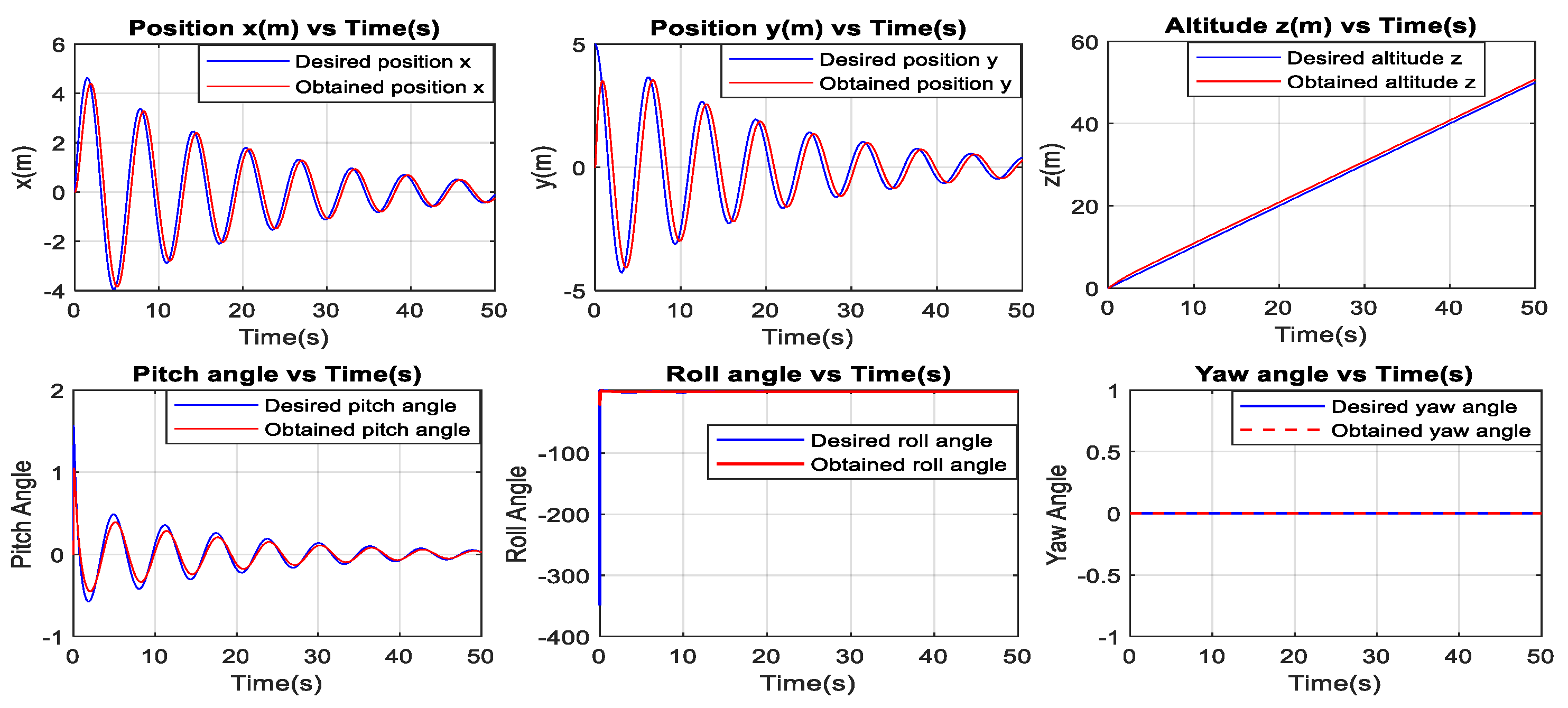
Using the PID gains derived from the linear model as a starting point, we fine-tuned the PID controller for the nonlinear model and obtained the following results shown in Figure 5:
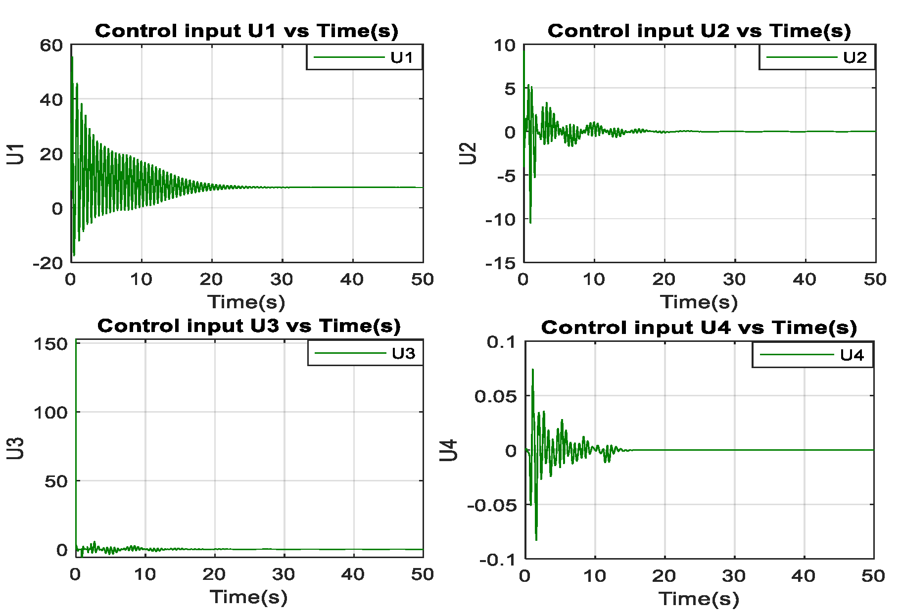
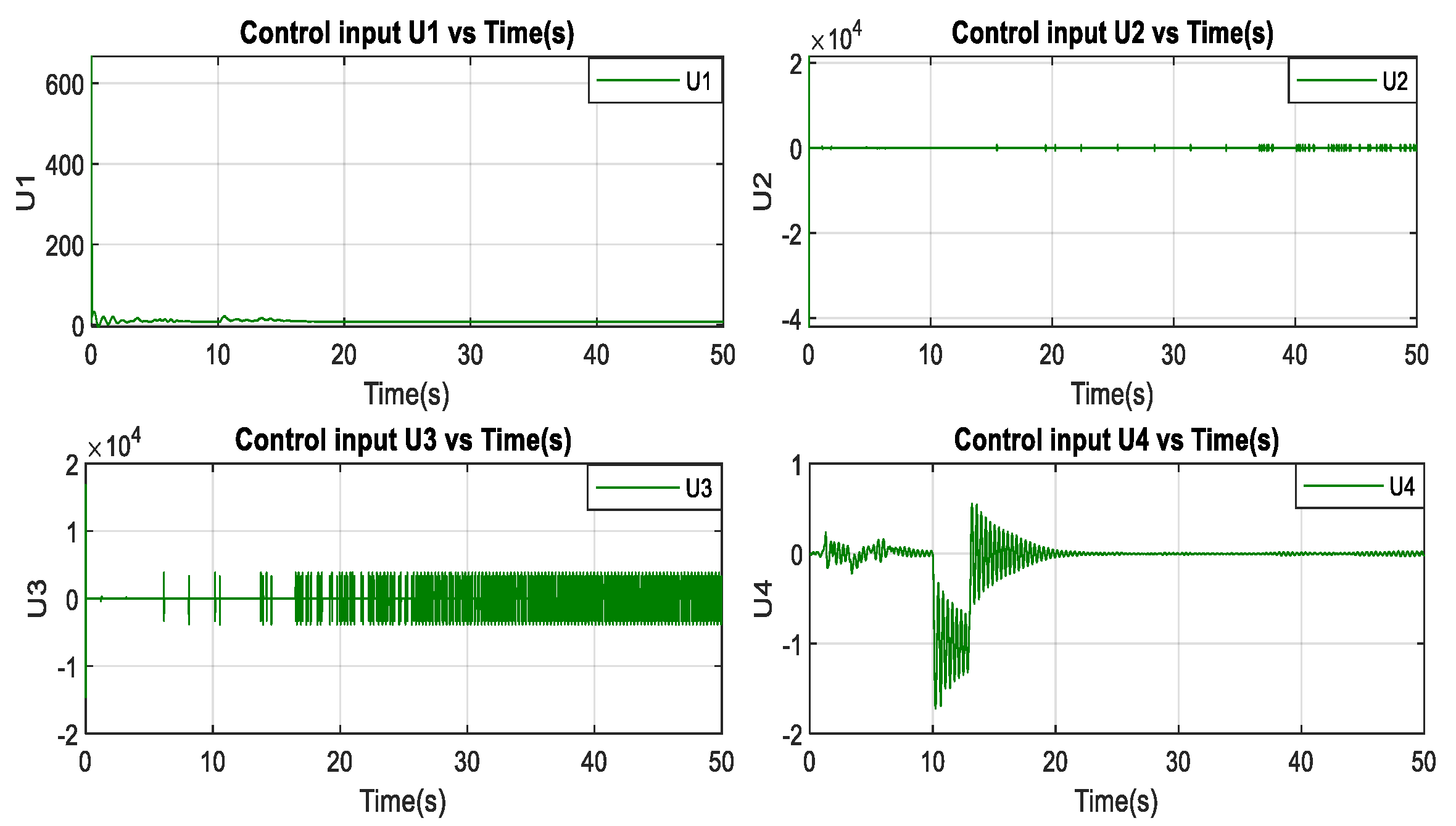
Figure 6 illustrates the control inputs from the PID controller without disturbance.
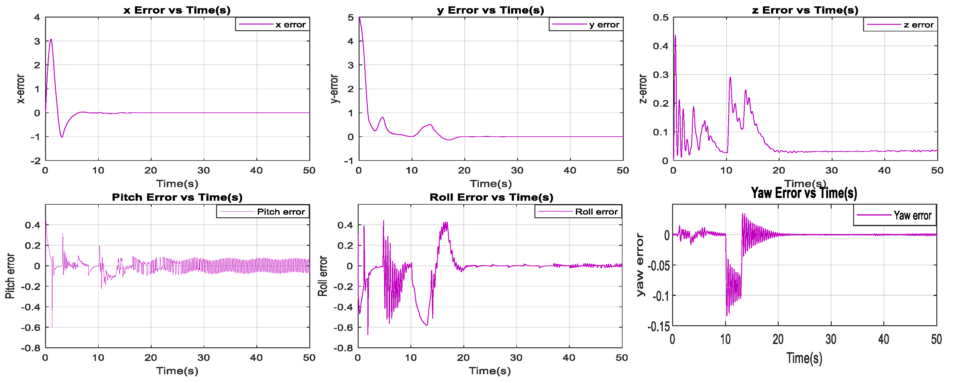
Figure 7 shows how the errors of positions x, y, and z and orientations roll, pitch, and yaw change with respect to time.
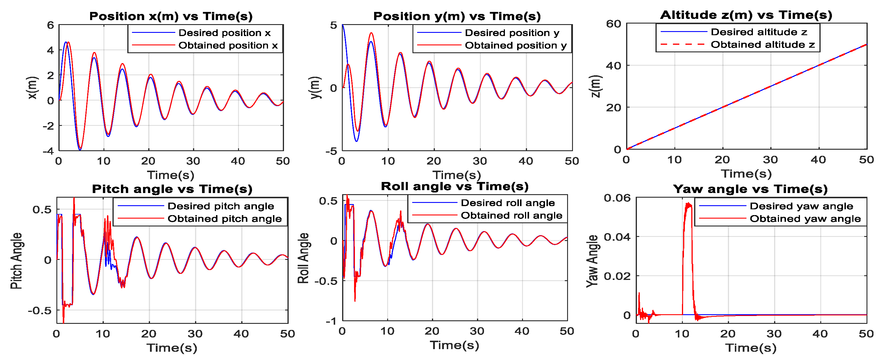
Disturbance was introduced to the closed loop system in the interval t = {10 s–13 s}. The results are shown in Figure 8.
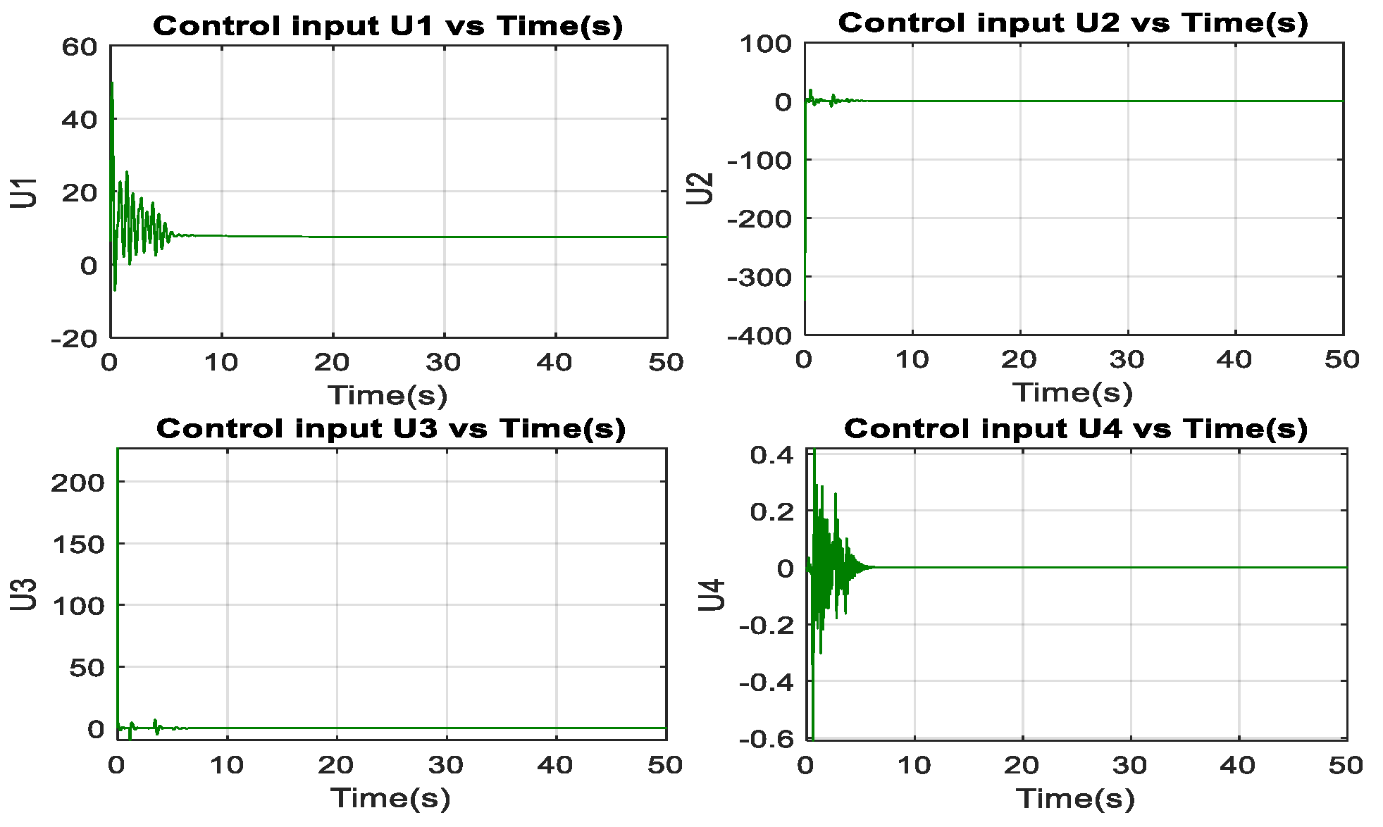
Figure 9 illustrates the control inputs from the PID controller with a disturbance.
Figure 10 shows how the errors of positions x, y, and z and orientations roll, pitch, and yaw change with respect to time:

3.4.2. Fractional-Order PID Controller Results

The initial gains were obtained from the PID controller for the nonlinear model. Subsequently, these gains were further adjusted to optimize the performance of the fractional-order PID controller. The evaluation of the fractional-order PID controller was carried out under both disturbance and non-disturbance conditions to highlight its adaptability and effectiveness in handling external influences. The following section dives into the results of these simulations, providing insights into the performance and robustness of the fractional-order PID controller in real-world scenarios. Table 4 displays the fractional-order PID controller gains for positions x, y, and z and orientations roll, pitch, and yaw, as well as the parameters µ and λ. These optimized gains are essential in ensuring accurate and stable control of the system, allowing the fractional-order PID controller to regulate the trajectory effectively under the influence of nonlinear dynamics.
Figure 11 shows some modifications of the gains obtained from the previous PID controller and by tuning the parameters of the fractional-order PID controller.
Figure 12 depicts the control inputs from the fractional-order PID controller without disturbance.
Figure 13 shows how the errors of positions x, y, and z and orientations roll, pitch, and yaw change with respect to time.
After introducing disturbance to the closed loop system in the interval t={10s-13s}, the following results shown in Figure 14 were obtained:
Figure 15 depicts the control inputs from the FOPID controller with disturbance.
Figure 16 shows how the errors of positions x, y, and z and orientations roll, pitch, and yaw change with respect to time.

3.4.3. Sliding Mode Controller Results

The simulation of the sliding mode controller starts with initial gains set to “ones”, which is then fine-tuned to achieve optimal values, ensuring the controller’s robustness and adaptability. Through a comprehensive exploration of various scenarios, with and without disturbances, we examine the controller’s adeptness in regulating trajectory outputs and ensuring system stability. This section presents a detailed analysis of the simulation results, providing valuable insights into the sliding mode controller’s efficiency in handling intricate dynamics and external perturbations. Table 5 displays the sliding mode gains for positions x, y, and z, and orientations roll, pitch, and yaw for the nonlinear model.
These optimized gains are essential in ensuring accurate and stable control of the system, allowing the sliding mode controller to regulate the trajectory effectively under the influence of nonlinear dynamics.
Through careful adjustment of the gains, the results presented in Figure 17 demonstrate effective and stable control in the absence of disturbances. These outcomes serve as proof of the sliding mode controller’s adaptability in successfully handling nonlinear dynamics.
Figure 18 depicts the control inputs from a sliding mode controller without disturbance.
Figure 19 shows how the errors of positions x, y, and z and orientations roll, pitch, and yaw change with respect to time.
Despite the presence of disturbances, the sliding mode controller in Figure 20 demonstrates exceptional adaptability by effectively handling nonlinear dynamics, maintaining stability, and achieving precise trajectory tracking.
Figure 21 depicts the control inputs from the SMC with the presence of disturbance.
Figure 22 displays how the errors of positions x, y, and z and orientations roll, pitch, and yaw change with respect to time.

3.5. Discussion

Each controller has its advantages and suitability for specific applications. The PID controller is reliable and widely used, while the fractional-order PID controller provides enhanced flexibility. Meanwhile, the sliding mode controller excels in handling disturbances and uncertainties. The choice of the controller depends on the specific requirements and characteristics of the control system. Further research and experimentation are encouraged to explore these controllers’ performance in different applications and real-world scenarios.
The PID controller, originally designed for the linear model, initially exhibited a slight perturbation in trajectory due to a disparity between the desired y trajectory’s starting point (set at 5) and the quadcopter’s actual initial position (which is 0). Additionally, a minor delay of approximately 1 s was observed in trajectory tracking, which was attributed to the system’s inherent oscillatory behavior. When applied to the nonlinear model, the PID controller displayed an initial time lag aligning with the trajectory. It manifested noticeable perturbations at the beginning of the trajectory: around 14 s for the x component and 5 s for the y component. However, beyond this initial phase, the controller gradually stabilized, closely approaching the desired path, while exhibiting a slight delay and a minor error. The PID controller demonstrated an acceptable performance in handling disturbances. It effectively managed the impact of disturbances on the y component. However, it exhibited a delayed reaction in addressing the deviations in the x component. It is worth noting the consistent presence of a delay in trajectory tracking, as well as a minor error that persisted along the trajectory. Regarding the altitude and heading components, the PID controller’s performance was notably satisfactory both in the presence and absence of disturbances. Despite these observations, the PID controller’s handling of disturbances remained acceptable overall.

3.6. Comparison

After evaluating the PID, fractional-order PID (FOPID), and sliding mode controllers for trajectory tracking, distinct performance characteristics came to light: The PID controller displayed effective disturbance handling even though there were considerable delays and overshoots. The fractional-order PID controller exhibited remarkable performance in rejecting disturbances; however, there is still some presence of error.
On the contrary, the sliding mode controller excelled comprehensively. The sliding mode controller not only achieved accurate trajectory tracking with minimal delays but also robustly handled disturbances, maintained minimal errors, achieved quick settling times, and demonstrated negligible overshoot. Taking these attributes into account, the sliding mode controller emerges as the most efficient choice, showcasing exceptional performance and suitability for achieving precise and effective trajectory tracking across many scenarios.
This section has provided a comprehensive evaluation of three controllers: PID, fractional-order PID, and sliding mode.
The PID controller demonstrated reliability and adaptability, yet with delays and overshoots. The fractional-order PID exhibited potential and robustness, but there were still slight errors present, along with initial instability. In contrast, the sliding mode controller stood out with precise trajectory tracking, robust disturbance handling, rapid settling times, and minimal overshoot.
This exceptional performance positions the sliding mode controller as the preferred choice for real-world applications requiring accurate trajectory tracking and offering valuable insights for practical implementation.
When controlling a quadcopter, the PID, FOPID, and sliding mode controllers (SMCs) offer different advantages and challenges. The PID controller is simple and widely used but struggles with nonlinearities and disturbances. The FOPID controller, with fractional calculus, provides better flexibility and robustness but is complex to design and computationally intensive. The SMC excels in robustness and handling nonlinearities, making it ideal for quadcopters, but it suffers from implementation complexity and chattering issues. The choice of control method hinges on balancing performance requirements, system complexity, and implementation feasibility.

4. Enhancing Quadcopter Trajectory Tracking through Dyna-Q Learning

Trajectory planning and obstacle avoidance are important for quadcopter navigation, ensuring safe and efficient paths in complex environments. By employing reinforcement learning, particularly the Dyna-Q approach, quadcopters can enhance their decision-making and adapt their flight trajectories. This combination of strategic path planning and adaptive obstacle avoidance, aided by advanced machine learning, allows quadcopters to optimize their operations, prevent collisions, and maintain stability while dynamically adjusting to their surroundings and achieving mission objectives [27,28,29,30,31].

4.1. Reinforcement Learning Approaches

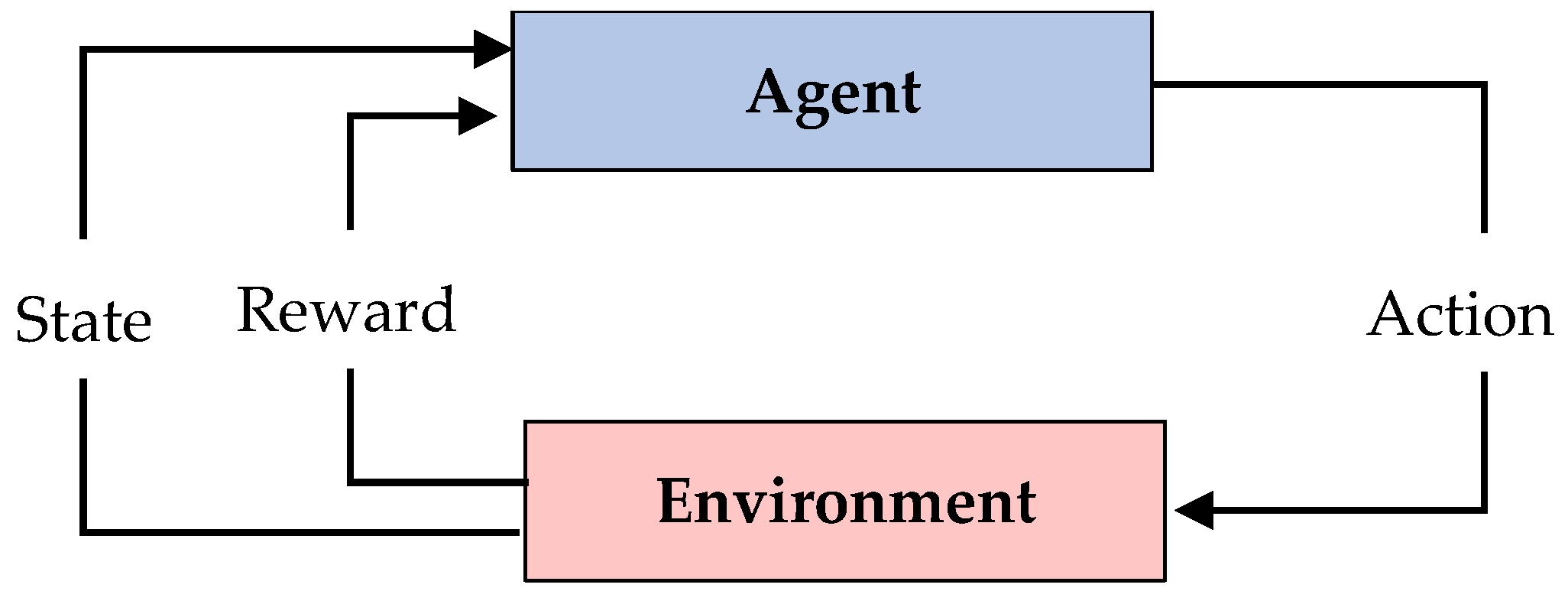
Reinforcement learning is a type of machine learning approach where an agent learns to make decisions by interacting with an environment [12,32]. Figure 23 shows the reinforcement learning block diagram.
The agent learns and makes decisions and takes actions to maximize cumulative rewards over time, adjusting its behavior based on the reward received from the environment that indicates how good or bad the actions were. This feedback loop helps the agent learn optimal strategies for achieving specific goals, making it well suited for tasks that involve sequential decision-making in dynamic environments [12,32].
Reinforcement learning approaches consist of model-free and model-based approaches. The model-based approach includes learning the model or being provided with the model, while the model-free approach involves policy optimization and Q-learning techniques. Dyna-Q learning combines both learning the model and Q-learning to optimize the learning process effectively. In reinforcement learning, the Markov Decision Process (MDP) is used to model the interactions between an agent and the environment, helping the agent maximize cumulative rewards in uncertain environments [12,27,29,32,33]. MDPs aim to determine policies that guide the agent’s actions:
-
The deterministic policy specifies a single action for each state; for every state (s) there is a clear action choice πSA that the agent follows.
-
The stochastic policy assigns a distribution over actions to each state following the policy π such that π: S → proba(A), where the agent decides actions based on probabilities for each state (s). This way, the agent can choose different actions in a state, with each option having its own chance of being selected.
Environments can also be deterministic (outcomes of actions are predictable) and stochastic (outcomes of actions are probabilistic and uncertain). Dyna-Q learning effectively navigates both deterministic and stochastic environments by optimizing the agent’s decision.

4.2. Q-Learning Algorithms

Q-learning is a useful technique for improving how quadcopters are controlled. Scientists have tried different versions of Q-learning to solve issues in quadcopter control, such as not often receiving rewards or dealing with complicated situations. By using Q-learning, quadcopters can quickly change how they act, deal with different situations, and perform tasks on their own. This has the potential to enable these aerial robots to perform more advanced tasks in the future. The Q-learning technique leads the quadcopter to the development of a value function that helps make smart decisions based on the rewards they expect to receive [28,30,33,34,35].
The Q-value (s, a) estimates the expected reward starting from state (s), taking action (a), and following policy π, while the V-function Vπ(s) estimates the cumulative reward starting from state (s) under policy π. The optimal policy π∗ maximizes the expected cumulative rewards. The agent faces the exploration–exploitation dilemma, where it must balance trying new actions (exploration) to learn about the environment and selecting known actions (exploitation) to maximize rewards. The epsilon-greedy strategy manages this balance by occasionally choosing random actions to explore while mostly selecting the best-known actions. This process continuously updates the Q-values, guiding the agent towards optimal decisions.
In the domain of reinforcement learning, the temporal difference (TD) error plays a crucial role in updating the expected return of an agent’s actions as it transitions from one state to another. The TD error captures the difference between the current estimate of the Q-value of a state–action pair and the updated estimate based on observed outcomes. Mathematically, the TD error is defined as follows [12,28]:
T D   e r r o r = R ( s ,   a ) + γ   m a x   a   Q   ( s ,   a )   Q ( s ,   a )
The temporal difference (TD) update equation for Q-learning, which is a model-free reinforcement learning algorithm, is used to update the Q-values based on the observed rewards and transitions. The equations are as follows [15,34]:
Q ( s , a )       Q ( s , a ) + α T D
Q s , a       Q ( s , a ) + α ( R s ,   a + γ   m a x a   Q s ,   a Q ( s ,   a ) )
where α is the learning rate:
  • High Learning Rate (α near 1): The agent will be highly responsive to the most recent experiences.
  • Low Learning Rate (α near 0): The agent will be less responsive to new experiences and will rely more on existing knowledge.
Figure 24 shows the Q-learning algorithm block diagram.

4.3. Implementation of Dyna-Q Learning for Trajectory Planning

Reinforcement learning begins with an agent’s Q-table containing initial values. The agent explores and refines Q-values through interactions, guiding actions for higher rewards. Dyna-Q learning combines real experiences with simulations, helping the agent navigate complex environments efficiently by learning to avoid obstacles and achieve goals [10,12]. It maintains a Q-table and uses an environment model to accelerate learning. This approach strikes a balance between real and simulated experiences [15,16,34,35,36].
In reinforcement learning for optimal policy derivation, the Bellman equation for the state–value function V(s) is defined as follows:
V(s) = r(s) + γ  maxH T(s, a, s′) V(s′)
This leads to the Bellman equation for the action–value function:
Q(s, a) = r(s, a) + γH T(s, a, s′) [maxa Q(s′, a′)]
To create a transition matrix: T[s, a, s′] = P(s′ | s, a)
The agent’s possible states and actions are enumerated, and transition probabilities are assigned; the agent randomly selects an action while it is in a random state, then transitions to the next state according to the updated transition matrix, measures the reward according to the reward function, and updates the Q-values. This process is repeated in the m planning steps.
Figure 25 illustrates the Dyna-Q learning algorithm block diagram.
The TD (temporal difference) error for a state–action pair (s, a) in Dyna-Q is expressed as follows:
T D   e r r o r ( s ,   a ) = R ( s ,   a ) + γ   ( s T s ,   a ,   s m a x a   Q ( s ,   a ) ) Q ( s ,   a )
The temporal difference (TD) update equation for Q-learning is used to update the Q-values based on the observed rewards and transitions.
The equation becomes the following:
Q ( s ,   a )     Q ( s ,   a ) + α   [ R ( s ,   a ) + γ   ( Σ   s T s ,   a ,   s m a x a   Q ( s ,   a ) ) Q ( s ,   a ) ]
For obstacle avoidance:
-
A lower learning rate α is better for obstacle avoidance in uncertain environments. It allows the agent to be cautious in updating its Q-values based on new experiences.
-
A higher discount factor γ is better for obstacle avoidance. It encourages the agent to consider long-term consequences and plan for the future, which is important when navigating around obstacles and finding safe paths.
-
A lower exploration rate ε is better for obstacle avoidance during the initial stages of learning.

4.4. Results

Table 6 summarizes the chosen values of the parameters used in the improved Dyna-Q learning algorithm.

4.4.1. Deterministic and Stochastic Environments Results

Real-world environments often have some level of uncertainty, and incorporating stochastic elements in the learning process can be beneficial to train agents that perform well in uncertain and dynamic scenarios. Ultimately, the choice between deterministic and stochastic environments depends on the application and the learning goals.
The total reward and steps in the deterministic environment are shown in Figure 26.
The trajectory path planning is represented in Figure 27 in 2D and 3D spaces.
The total reward and steps in the stochastic environment are shown in Figure 28.
The trajectory path planning is represented in 2D and 3D spaces in Figure 29.
The stochastic environment seems to yield a more direct path from the starting point to the goal while avoiding obstacles effectively. This could be because the stochastic environment encourages the agent to explore and find efficient paths rather than taking a roundabout route. If this behavior aligns with your goals and the real-world scenario you are simulating, the stochastic environment might be more appropriate.

4.4.2. Dyna-Q Learning with Sliding Mode Controller

After using the path determined by Dyna-Q learning as the planned path and employing a sliding mode controller to manage the quadcopter’s movements, the resulting flight path can be observed in both 3D and 2D spaces in Figure 30.
Table 7 displays the sliding mode gains for positions x, y, and z and orientations roll, pitch, and yaw for the obtained trajectory from using Dyna-Q learning.
The following results in Figure 31 were obtained:
Figure 32 depicts the control inputs from the sliding mode controller.
Figure 33 shows how the errors of positions x, y, and z and orientations roll, pitch, and yaw change with respect to time.

4.5. Discussion

The obtained results from the integration of the sliding mode controller with the Dyna-Q learning-based obstacle avoidance system were indeed remarkable. The Dyna-Q learning agent demonstrated impressive performance in learning optimal collision-free paths for the quadcopter in complex environments. Through iterations of simulation and interaction with various obstacles, the agent effectively applied a set of trajectories that enabled safe and efficient navigation. Employing these learned trajectories as the desired path for the quadcopter, the sliding mode controller showcased its ability to accurately track the trajectory, maintaining a high level of precision.
The sliding mode controller offers an excellent solution for trajectory planning and obstacle avoidance due to its robustness, adaptability, and ability to manage constraints. Its inherent capability to swiftly adjust control inputs to follow optimized trajectories, as demonstrated by its integration with Dyna-Q learning for obstacle avoidance, makes it a prime choice for achieving high-performance autonomous navigation. The SMC’s capacity to ensure accurate and safe trajectory tracking, even in the presence of disturbances and uncertainties, makes it a key choice for enhancing the capabilities of autonomous systems operating in complex and obstacle-rich environments.
At last, the integration of Dyna-Q learning and the sliding mode controller presents a powerful solution for obstacle avoidance in autonomous quadcopter navigation. This approach, driven by data-driven reinforcement learning and robust real-time control, demonstrates remarkable efficiency, safety, and adaptability. By enabling quadcopters to learn optimal trajectories and swiftly respond to dynamic environments, this approach holds great promise for enhancing quadcopter autonomy and successfully navigating intricate space.

5. Conclusions

The objective of this study was to formulate a precise mathematical model for a quadcopter and to devise three distinct control strategies: linear PID, nonlinear fractional-order PID, and sliding mode controllers, with the aim of stabilizing the quadcopter’s behavior. Through extensive simulations and precisely refining these controllers, important results were concluded. Remarkably, the fractional-order PID controller demonstrated superior performance compared to the conventional PID controller when it came to accurately tracking flight paths that exhibited dynamic changes. Additionally, the sliding mode controller showcased exceptional proficiency in handling the complexities of nonlinear dynamics and external disturbances. The utilization of the sliding mode controller extended to trajectory planning. Notably, through the integration of Dyna-Q learning, the quadcopter’s navigational capabilities were augmented, setting the stage for enhanced autonomous navigation. Since the sliding mode controller (SMC) offered the best results among the three controllers in nonlinearity handling, it was chosen to be combined with Dyna-Q learning for quadcopter trajectory planning. Together, the SMC’s precise control and Dyna-Q’s adaptive planning create a powerful system for achieving efficient and reliable trajectory planning in dynamic environments.
In essence, this study successfully accomplished its dual objectives by formulating an adept mathematical model for the quadcopter and introducing three controllers. The fractional-order PID controller emerged as a frontrunner in adapting to varying flight paths, while the sliding mode controller excelled in managing complexities. This study’s insights contribute to the advancement of both quadcopter control methodologies and trajectory planning, with potential applications in autonomous aerial navigation.

Author Contributions

All authors contributed in all parts of this work (All authors worked as a group). All authors have read and agreed to the published version of the manuscript.

Funding

This research received no external funding.

Data Availability Statement

Data is contained within the article.

Conflicts of Interest

The authors declare no conflict of interest.

References

  1. Ahirwar, S.; Swarnkar, R.; Bhukya, S.; Namwade, G. Application of Drone in Agriculture. Int. J. Curr. Microbiol. Appl. Sci. 2019, 8, 2500–2505. [Google Scholar] [CrossRef]
  2. Kille, T.; Bates, P.R.; Lee, S.Y. Unmanned Aerial Vehicles in Civilian Logistics and Supply Chain Management; IGI Global: Hershey, PA, USA, 2019; pp. 66–67. [Google Scholar] [CrossRef]
  3. Raundal, A.; Dhawale, A.; Gathe, M.; Salunke, G. Fire Ball Drone. Int. J. Res. Publ. Rev. 2022, 3, 4055–4064. Available online: https://ijrpr.com/uploads/V3ISSUE6/IJRPR5298.pdf (accessed on 13 May 2024).
  4. Ostojić, G.; Stankovski, S.; Tejic, B.; Đukić, N.; Tegeltija, S. Design, Control and Application of Quadcopter. Int. J. Ind. Eng. Manag. (IJIEM) 2015, 6, 44–45. [Google Scholar] [CrossRef]
  5. Thu, K.M.; Gavrilov, A.I. Designing and modeling of quadcopter control system using L1 adaptive control. Procedia Comput. Sci. 2017, 103, 528–535. [Google Scholar] [CrossRef]
  6. Eatemadi, M. Mathematical Dynamics, Kinematics Modeling and PID Equation Controller of Quadcopter. Int. J. Appl. Oper. Res. 2017, 7, 77–85. Available online: http://ijorlu.liau.ac.ir/article-1-503-fa.html (accessed on 13 May 2024).
  7. Harkare, O.; Maan, R. Design and Control of a quadcopter. Int. J. Eng. Tech. Res. 2021, 10, 258. [Google Scholar] [CrossRef]
  8. Okulski, M.; Ławryńczuk, M. How Much Energy Do We Need to Fly with Greater Agility? Energy Consumption and Performance of an Attitude Stabilization Controller in a Quadcopter Drone: A Modified MPC vs. PID. Energies 2022, 15, 1380. [Google Scholar] [CrossRef]
  9. Yao, W.-S.; Lin, C.-Y. Dynamic Stiffness Enhancement of the Quadcopter Control System. Electronics 2022, 11, 2206. [Google Scholar] [CrossRef]
  10. Leitão, D.; Cunha, R.; Lemos, J.M. Adaptive Control of Quadrotors in Uncertain Environments. Eng 2024, 5, 544–561. [Google Scholar] [CrossRef]
  11. Li, J.; Chen, P.; Chang, Z.; Zhang, G.; Guo, L.; Zhao, C. Trajectory Tracking Control of Quadrotor Based on Fractional-Order S-Plane Model. Machines 2023, 11, 672. [Google Scholar] [CrossRef]
  12. Ademola, A.; Ademola, I.; Oguntosin, V.; Olawale, P. Modeling and Nonlinear Control of a Quadcopter for Stabilization and Trajectory Tracking. SSRN Electron. J. 2022. [Google Scholar] [CrossRef]
  13. Yih, C.-C.; Wu, S.-J. Sliding Mode Path following and Control Allocation of a Tilt-Rotor Quadcopter. Appl. Sci. 2022, 12, 11088. [Google Scholar] [CrossRef]
  14. Huo, X.; Zhang, T.; Wang, Y.; Liu, W. Dyna-Q Algorithm for Path Planning of Quadrotor UAVs. In Methods and Applications for Modeling and Simulation of Complex Systems. AsiaSim 2018. Communications in Computer and Information Science; Li, L., Hasegawa, K., Tanaka, S., Eds.; Springer: Singapore, 2018; Volume 946. [Google Scholar] [CrossRef]
  15. Budiyanto, A.; Matsunaga, N. Deep Dyna-Q for Rapid Learning and Improved Formation Achievement in Cooperative Transportation. Automation 2023, 4, 210–231. [Google Scholar] [CrossRef]
  16. Faycal, T.; Zito, C. Dyna-T: Dyna-Q and Upper Confidence Bounds Applied to Trees. arXiv 2022, arXiv:2201.04502. [Google Scholar]
  17. Changliu, Z.; Ding, X.; Yu, Y.; Wang, X. Quaternion-based Nonlinear Trajectory Tracking Control of a Quadrotor Unmanned Aerial Vehicle. Chin. J. Mech. Eng. 2017, 30, 84–85. [Google Scholar]
  18. Fernando, H.C.T.E.; De Silva, A.T.A.; De Zoysa, M.D.C.; Dilshan, K.A.D.C.; Munasinghe, S.R. Modelling, simulation and implementation of a quadrotor UAV. In Proceedings of the IEEE 8th International Conference on Industrial and Information Systems (ICIIS), Peradeniya, Sri Lanka, 17–20 December 2013; p. 207. [Google Scholar]
  19. Nagaty, A.; Saeedi, S.; Thibault, C.; Seto, M.; Li, H. Control and navigation framework for quadrotor helicopters. J. Intell. Robot. Syst. 2013, 69, 2–5. [Google Scholar] [CrossRef]
  20. Zheng, Q.; Tang, R.; Gou, S.; Zhang, W. A PID Gain Adjustment Scheme Based on Reinforcement Learning Algorithm for a Quadrotor. In Proceedings of the 39th Chinese Control Conference (CCC), Shenyang, China, 27–29 July 2020. [Google Scholar]
  21. Siti, I.; Mjahed, M.; Ayad, H.; El Kari, A. New Designing Approaches for Quadcopter PID Controllers Using Reference Model and Genetic Algorithm Techniques. Int. Rev. Autom. Control (IREACO) 2017, 10, 240–248. [Google Scholar] [CrossRef]
  22. Bingi, K.; Ibrahim, R.; Karsiti, M.N.; Hassan, S.M. Fractional-order Systems and PID Controllers Using Scilab and Curve Fitting Based Approximation Techniques. In Studies in Systems, Decision and Control; Springer: Berlin/Heidelberg, Germany, 2020; Volume 264. [Google Scholar]
  23. Mirghasemi, S.A. Fractional Order Controller for Quadcopter Subjected to Ground Effect. Master’s Thesis, University of Ottawa, Ottawa, ON, Canada, 2019; pp. 14–15. [Google Scholar] [CrossRef]
  24. Le, H.D.; Nestorović, T. Adaptive Proportional Integral Derivative Nonsingular Dual Terminal Sliding Mode Control for Robotic Manipulators. Dynamics 2023, 3, 656–677. [Google Scholar] [CrossRef]
  25. Loubar, H.; Boushaki, R.; Aouati, A.; Bouanzoul, M. Sliding Mode Controller for Linear and Nonlinear Trajectory Tracking of a Quadrotor. Int. Rev. Autom. Control (IREACO) 2020, 13, 128–138. [Google Scholar] [CrossRef]
  26. Elagib, R.; Karaarslan, A. Sliding Mode Control-Based Modeling and Simulation of a Quadcopter. J. Eng. Res. Rep. 2023, 24, 32–41. [Google Scholar] [CrossRef]
  27. Ling, F.; Jimenez-Rodriguez, A.; Prescott, T.J. Obstacle Avoidance Using Stereo Vision and Deep Reinforcement Learning in an Animal-like Robot. In Proceedings of the International Conference on Robotics and Biomimetics (ROBIO), Dali, China, 6–8 December 2019; pp. 1–94. [Google Scholar]
  28. Deshpande, A.M.; Minai, A.A.; Kumar, M. Robust Deep Reinforcement Learning for Quadcopter Control. IFAC-PaperOnLine 2021, 54, 90–95. [Google Scholar] [CrossRef]
  29. Lambert, N.O.; Drew, D.S.; Yaconelli, J.; Levine, S.; Calandra, R.; Pister, K.S.J. Low-Level Control of a Quadrotor with Deep Model-Based Reinforcement Learning. IEEE Robot. Autom. Lett. 2019, 4, 4224–4230. [Google Scholar] [CrossRef]
  30. Chen, D.; Wei, Y.; Wang, L.; Hong, C.S.; Wang, L.-C.; Han, Z. Deep Reinforcement Learning Based Strategy for Quadrotor UAV Pursuer and Evader Problem. In Proceedings of the IEEE International Conference on Communications Workshops, Dublin, Ireland, 7–11 June 2020. [Google Scholar] [CrossRef]
  31. Ouahouah, S.; Bagaa, M.; Prados-Garzon, J. Deep Reinforcement Learning based Collision Avoidance in UAV Environment. IEEE Internet Things J. 2022, 9, 4015–4030. [Google Scholar] [CrossRef]
  32. Agarwal, M.; Aggarwal, V.; Ghosh, A.; Tiwari, N. Reinforcement Learning for Mean-Field Game. Algorithms 2022, 15, 73. [Google Scholar] [CrossRef]
  33. Dhuheir, M.; Baccour, E.; Erbad, A.; Al-Obaidi, S.S.; Hamdi, M. Deep Reinforcement Learning for Trajectory Path Planning and Distributed Inference in Resource-Constrained UAV Swarms. IEEE Internet Things J. 2022, 10, 8185–8201. [Google Scholar] [CrossRef]
  34. Rubi, B.; Morcego, B.; Perez, R. A Deep Reinforcement Learning Approach for Path Following on a Quadrotor. In Proceedings of the European Control Conference (ECC), Saint Petersburg, Russia, 12–15 May 2020. [Google Scholar] [CrossRef]
  35. Yoo, J.; Jang, D.; Kim, H.J.; Johansson, K.H. Hybrid reinforcement learning control for a micro quadrotor flight. IEEE Control Syst. Lett. 2021, 5, 505–510. [Google Scholar] [CrossRef]
  36. Liu, H.; Zhao, W.; Lewis, F.L.; Jiang, Z.-P.; Modares, H. Data-based Formation Control for Underactuated Quadrotor Team via Reinforcement Learning*. In Proceedings of the 39th Chinese Control Conference (CCC), Shenyang, China, 27–29 July 2020. [Google Scholar] [CrossRef]
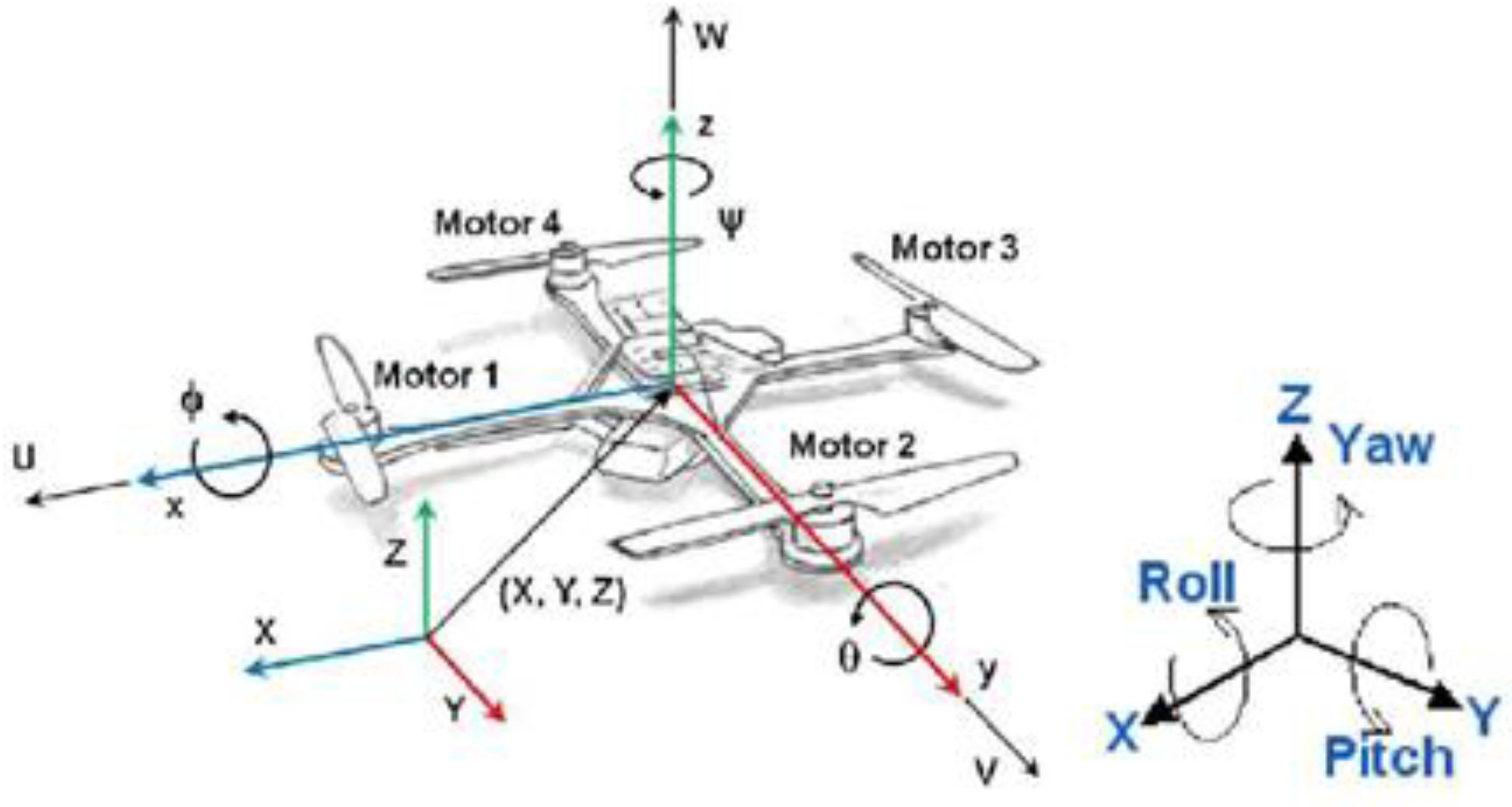
Figure 1. Movement of a quadcopter: body frame and inertial frame.
Automation 05 00010 g001
Figure 2. Desired and obtained trajectory simulation using the PID controller for the linear model.
Automation 05 00010 g002
Figure 3. Control inputs of the PID controller simulation for the linear model.
Automation 05 00010 g003
Figure 4. Errors in positions and orientations for the linear model using the PID controller.
Automation 05 00010 g004
Figure 5. Desired and obtained trajectory simulation using the PID controller for the nonlinear model without disturbance.
Automation 05 00010 g005
Figure 6. Control inputs of the PID controller simulation for the nonlinear model without disturbance.
Automation 05 00010 g006
Figure 7. Errors in positions and orientations in the nonlinear model using the PID controller without disturbance.
Automation 05 00010 g007
Figure 8. Desired and obtained trajectory simulation using the PID controller for the nonlinear model with disturbance.
Automation 05 00010 g008
Figure 9. Control inputs of the PID controller simulation for the nonlinear model with disturbance.
Automation 05 00010 g009
Figure 10. Errors in positions and orientations for the nonlinear model using the PID controller with disturbance.
Automation 05 00010 g010
Figure 11. Desired and obtained trajectory simulation using the FOPID controller without disturbance.
Automation 05 00010 g011
Figure 12. Control inputs of the FOPID controller simulation for the nonlinear model without disturbance.
Automation 05 00010 g012
Figure 13. Errors in positions and orientations for the nonlinear model using the FOPID controller without disturbance.
Automation 05 00010 g013
Figure 14. Desired and obtained trajectory simulation using the FOPID controller with disturbance.
Automation 05 00010 g014
Figure 15. Control inputs of the FOPID controller simulation for the nonlinear model with disturbance.
Automation 05 00010 g015
Figure 16. Errors in positions and orientations for the nonlinear model using the FOPID controller with disturbance.
Automation 05 00010 g016
Figure 17. Desired and obtained trajectory simulation using the SMC without disturbance.
Automation 05 00010 g017
Figure 18. Control inputs of the SMC simulation for the nonlinear model without disturbance.
Automation 05 00010 g018
Figure 19. Errors in positions and orientations for the nonlinear model using the SMC without disturbance.
Automation 05 00010 g019
Figure 20. Desired and obtained trajectory using the SMC with disturbance.
Automation 05 00010 g020
Figure 21. Control inputs of the SMC simulation for the nonlinear model with disturbance.
Automation 05 00010 g021
Figure 22. Errors in positions and orientations for the nonlinear model using the SMC with disturbance.
Automation 05 00010 g022
Figure 23. Reinforcement learning block diagram.
Automation 05 00010 g023
Figure 24. Q-learning algorithm block diagram.
Automation 05 00010 g024
Figure 25. Dyna-Q learning algorithm block diagram.
Automation 05 00010 g025
Figure 26. Total reward and total steps per episode for the deterministic environment.
Automation 05 00010 g026
Figure 27. The 2D and 3D deterministic environment path planning (The red squares: obstacles, the blue line: the optimal path).
Automation 05 00010 g027
Figure 28. Total reward and total steps per episode for the stochastic environment.
Automation 05 00010 g028
Figure 29. The 2D and 3D stochastic environment path planning (The red squares: obstacles, the blue line: the optimal path).
Automation 05 00010 g029
Figure 30. The 2D and 3d quadcopter trajectory using the sliding mode controller (The red squares: obstacles, the blue line: the optimal path).
Automation 05 00010 g030
Figure 31. Desired and obtained trajectory using the SM controller.
Automation 05 00010 g031
Figure 32. Control inputs of the sliding mode controller simulation.
Automation 05 00010 g032
Figure 33. Errors in positions and orientations using the sliding mode controller.
Automation 05 00010 g033
Table 1. Extended types of classical PID controllers.
Type of Controllerλμ
P I λ 0 < λ < 10
P I λ D 0 < λ < 11
P D μ 0 0 < μ < 1
P I D μ 1 0 < μ < 1
P I λ D μ 0 < λ < 1 0 < μ < 1
Table 2. PID controller gains, settling time, and overshoot for the linear model.
ControllerPIDSettling TimeOvershoot
x0.188580.00254213.10821.28 s0.737%
y0.381070.00534183.22454.95 s4.42%
z110.034082150.863 s2.61%
Roll0.25640.0259260.56345.15 s5.58%
Pitch0.97880.192951.10330.001 s4.25%
Yaw3.26825.50530.22350.9098.07%
Table 3. PID controller gains for the nonlinear model.
PIDPID
x0.250.0033.5
y0.920.012
z1505030
Roll90.051.2
Pitch70.21
Yaw3.265.50.22
Table 4. FOPID controller gains for the nonlinear model.
FOPIDKPKIKDλμ
x10.01150.80.785
y10.0140.80.64
z140503011
Roll10.031.90.60.8
Pitch10.210.50.8
Yaw3.265.510.80.9
Table 5. The SMC gains for the nonlinear model.
ControllerλK1K2
x100.50.9
y14.50.11.5
z50.110
ϕ 10.20.17.5
θ 50.01110
ψ 300.130
Table 6. The values of the parameters used in the improved Dyna-Q learning algorithm.
Number of EpisodesLearning RateDiscount FactorExploration RateHorizonObstacle Hit
Reward
Reach Goal
Reward
Regular
Step
30000.10.80.2200−100100−2
Table 7. SM gains for the resulting path from Dyna-Q learning.
ControllerλK1K2
x1.50.080.4
y1.60.070.6
z0.50.0860
ϕ 400.514
θ 490.311
ψ 0.514
Disclaimer/Publisher’s Note: The statements, opinions and data contained in all publications are solely those of the individual author(s) and contributor(s) and not of MDPI and/or the editor(s). MDPI and/or the editor(s) disclaim responsibility for any injury to people or property resulting from any ideas, methods, instructions or products referred to in the content.