Article

Deep Learning-Based Detection and Segmentation of Damage in Solar Panels

by
Ayesha Shaik
1,2,
Ananthakrishnan Balasundaram
1,2,*,
Lakshmi Sairam Kakarla
2 and
Nivedita Murugan
2
1
Centre for Cyber Physical Systems, Vellore Institute of Technology, Chennai 600127, India
2
School of Computer Science and Engineering, Vellore Institute of Technology, Chennai 632014, India
*
Author to whom correspondence should be addressed.
Automation 2024, 5(2), 128-150; https://doi.org/10.3390/automation5020009
Submission received: 6 March 2024 / Revised: 27 May 2024 / Accepted: 28 May 2024 / Published: 29 May 2024

Abstract

:
Renewable energy can lead to a sustainable future and solar energy is one the primary sources of renewable energy. Solar energy is harvested mainly by photovoltaic plants. Though there are a large number of solar panels, the economic efficiency of solar panels is not that high in comparison to energy production from coal or nuclear matter. The main risk involved in solar plants is the high maintenance cost involved in maintaining the plants. To help reduce this issue, automated solutions using Unmanned Aerial Vehicles (UAVs) and satellite imagery are proposed. In this research work, we propose a novel deep learning architecture for the segmentation of solar plant aerial images, which not only helps in automated solar plant maintenance, but can also be used for the area estimation and extraction of solar panels from an image. Along with this, we also propose a transfer learning-based model for the efficient classification of solar panel damage. Solar panel damage classification has a lot of applications. It can be integrated into monitoring systems, raising alerts when there is severe damage or damage of a certain type. The adaptive UNet model with Atrous Spatial Pyramid Pooling (ASPP) module that performed the dilated convolutions that we proposed achieved an overall accuracy of 98% with a Mean Intersection-Over-Union (IoU) Score of 95% and took under a second to process an image. Our classification model using Visual Geometry Group 19 (VGG19) as the backbone for feature extraction has achieved a classification accuracy of 98% with an F1 score of 99%, thus detecting the five classes of damage, including undamaged solar panels, in an efficient manner.

1. Introduction

Renewable energy has always piqued humanity’s interest. Given the problems of global warming and finite fossil fuel reserves, everyone is looking for a dependable and renewable energy source. Renewable energy has the potential to replace carbon-based fossil fuels as the primary energy source for future cities. Given recent rapid global urbanization, it is now more important than ever to incorporate clean renewable energy sources in order to reduce environmental damage while also ensuring reliable and sustainable population growth in the coming decades. As a result, there has been a massive increase in renewable energy installations in recent years, including solar, wind, and geothermal energy facilities. This is especially noticeable when using electricity instead of natural fuels. Solar energy, wind energy, and hydro energy are the primary sources of renewable energy. Solar energy plants have numerous advantages, including increased longevity, environmental friendliness, quiet operation, and cleanliness.
With solar energy being a major source of renewable energy, the market for PV (photovoltaic) plants, also known as solar plants, is rapidly expanding. PV plant expansion has reached 35% in the last decade. According to the data, new solar installations account for 55% of this new capacity, with Asia accounting for 70%. GCC desert-climate countries like the UAE and Saudi Arabia are major solar energy investors in the region. With an average daily sunshine of 10 h per day and a Global Horizontal Irradiance index (GHI) of 2.12 MWh/m2/year, such countries have the potential to generate massive amounts of solar power, which could eventually replace their current reliance on carbon-based fossil fuels. Nonetheless, the integration of solar energy sources into main grids remains relatively low. In the United Arab Emirates, for example, 22.5 MW of installed solar capacity amounts to only 0.49% of total capacity. Despite the GCC’s recent exponential growth in new solar installations, a 100% renewable energy grid remains a long-term goal. This is primarily because desert solar installations face challenges such as overheating and soiling. As a result, significant research efforts have been devoted to improving and optimizing the performance of solar modules in such environments.
Because of the advent of new technologies, there is currently a lot of interest in autonomous monitoring for PV systems. Aerial robots have been used to inspect utility-scale PV plants in recent years. Many efforts have been expended in order to create a dependable and cost-effective aerial monitoring system for maximum productivity in PV plant inspection. The high return on investment of solar panels, as well as the low production costs of PV panels, are important factors in this. The market for PV plants is exploding as a result of the proposal of using carbon credits to reduce carbon emissions and thus global warming, as well as increased government subsidies around the world.
As usage grows, so does the need for upkeep. Major issues in PV plants include inverter failure due to voltage differences and poor PV module performance. A variety of factors can influence PV module performance. Among them are PV panel build quality, environmental conditions, installation location, and height. Because PV panels are typically installed on roofs or farms, expert maintenance is required under extremely demanding working conditions. Weather fluctuations reflect the intermittent nature of weather conditions, which can propagate through main girds, causing power planning inconvenience at best and critical asset damage at worst. Furthermore, solar modules are frequently installed in remote and harsh environments, making them vulnerable to environmental damage such as overheating, surface scratching, and material decay. Such faults can cause serious issues such as module mismatch or open circuits, significantly reducing an installation’s power output. Furthermore, once a solar installation is connected to the grid, it is critical that the system is always aware of the installation’s status and output in order to ensure reliable power planning. PV maintenance is frequently associated with high costs and a lengthy process. Professional personnel are expected to need up to 8 h to inspect each megawatt of power generated by the panels. This is one of the most important factors influencing PV plant growth.
Many tasks, including farm maintenance, delivery of goods, and high-altitude maintenance, have benefited greatly from the use of drones and UAVs (Unmanned Aerial Vehicles). A lot of work has been carried out that proposes the use of UAVs and drones to automate, at least to some extent, the maintenance of PV plants. As a result, research teams are currently working on developing equipment that can automatically inspect and clean PV systems. UAVs can enable automatic evaluation and tracking at a lower cost, cover larger areas, and detect threats faster than the traditional method of PV plant maintenance, which involves trained personnel manually inspecting and cleaning the surface of PV plants. UAVs (Unmanned Aerial Vehicles) have recently been proposed for PV inspections. Over the last few decades, research has made significant advances in the development of Unmanned Aerial Vehicles (UAVs) for monitoring applications such as power transmission lines, gas and oil pipeline inspection, precision agriculture, and bridge inspection. Indeed, the ability of multirotor UAVs to hover and freely move in the air, as well as the ease with which they can be piloted and outfitted with various sensors, makes this technology very appealing in monitoring scenarios.
UAV cameras photograph the area of the photovoltaic system, which can then be identified using image analysis in a process known as border extraction. Based on the estimated boundary, the UAVs can use CPP to compute a path to cover the panels (Coverage Path Planning). It is not possible to fly precisely over all of the PV plants. The path planning algorithm requires the maximum and minimum dimensions of the PV plants in both the horizontal and vertical axes. Based on the shape of the panel and the surrounding environment, a few points are identified as pivot points in CPP. To connect the pivot points and thus cover the PV panels, tracks are calculated. Once the CPP is completed, a flight zone is assigned to a UAV equipped with a GPS receiver and an Inertial Measurement Unit (IMU). The drone can cover the entire panel area and detect and repair some defects depending on the equipment installed in the UAV. PV plants which are partially covered in dust, snow, or leaves, for example, could be cleaned. UAVs can also detect and repair cracks in PV plants’ surfaces automatically. More manual maintenance areas can be identified, and the necessary maintenance can be automatically scheduled.
To improve monitoring accuracy during diagnosis using machine learning algorithms, massive amounts of data from various PV systems are required for autonomous monitoring. The maintenance of PV plants is critical to the profitability of energy production, and the autonomous inspection of such systems is a promising technology, particularly for large utility-scale plants where manned techniques face significant time, cost, and performance constraints. Sensors mounted on an aerial robot can capture typical aerial imagery consisting of RGB and infrared (IR) images during PV plant inspection to systematically detect the borders of PV plants.
The goal of this work is to develop a dependable and simple technique for identifying PV plant boundaries and detecting panel defects in comparison to the currently available techniques for detecting PV plant boundaries. Previous studies are concerned with establishing boundaries using advanced image processing techniques. This necessitates the use of a variety of filters and edge detection techniques. Because deep learning on images is currently so popular, newer works rely heavily on large and complex neural network architectures. The goal of this work is to combine the two major methods by applying image processing techniques to the data and developing a lightweight neural network to detect the boundaries based on the processed images.
It is well understood that any type of damage to the solar panel surface affects the efficiency of a solar panel. When even the solar panel is damaged, the amount of power it generates reduces; the extent of this reduction depends on the nature of the damage. There are many kinds of damage that a solar panel can experience. For instance, due to weather conditions, solar panels may be covered with snow, soil, cement, etc. Bird droppings on solar panels can not only cover the panel, but also damage the surface of the solar panel by reacting with the panel materials. Cracks on solar panels are very common; they may occur due to impacts from falling objects such as stones or even ice. Thus, for the effective monitoring of solar panels, having a damage detection system is vital.

1.1. Literature Review

Andres Perez et al. [1] proposed a deep learning-based model for boundary estimation. The major aim of their work was to predict a mask that semantically identified the PV panels in a given aerial image. They extensively discussed the various techniques used to solve this task of edge detection and showed how their implementation mostly overcame the drawbacks of the existing approaches. In terms of data, they worked on the “Amir” dataset. The input for their model was an RGB image captured by a UAV. The model predicted a set of ones and zeros equal to the dimensions of the input image. The high areas indicated the presence of a PV plant. Their model was able to achieve a mean IOU of around 90%, which is accurate enough. Yet, we find that there is scope for improvement here as well. In terms of the complexity of the model, they used a UNet implementation for this task. UNet is a state-of-the-art architecture for medical image semantic segmentation which has recently been widely used for other tasks as well. Sizkouhi et al. [2] proposed an encoder–decoder architecture for the detection of faults in PV plants. Their work majorly focused on identifying bird droppings on panels and estimating the severity of bird droppings on the performance of PV modules. Their encoder–decoder architecture is very similar to that of UNet; indeed, they both use VGG as a backbone. Though their task also involved identifying PV plants, not much data were provided on their efficiency while doing so. But they claim that their model was able to achieve a pixel accuracy of around 93% when identifying bird dropping areas on the panels. Based on the area of the patch, i.e., the number of pixels predicted to be bird droppings, they predicted the severity of the effects of the blockage on the PV modules’ performance.
Ramirez, Isacc et al. [3] proposed a novel condition monitoring system to accurately identify hot spots, i.e., possible fault areas, in PV panels. Their method achieved a testing accuracy of 93%. In their work, they used two ANNs for identifying the hot spots. They proposed an IOT platform approach that inputs the data from a thermal camera fitted on the UAV. The data from the UAV as well as the IoT platform equipped on the PV plants were used by two different neural networks to make predictions. Based on the output of the two models, they made predictions about the possible hot spots. Most of the approach is very similar to others in the literature, but the inclusion of the IoT platform gives some novelty to this approach. Shapsough et al. [4] worked on using IoT and deep learning to create a low-cost edge-based anomaly detection system. This system can remotely sense any outliers in the PV module’s performance and generate respective alerts. They used soil conditioning sensors to constantly collect and monitor data and used deep learning techniques to identify fluctuations based on these data. Sizkouhi et al. [5] created a framework called RoboPV. The major modules of this framework were boundary detection and CPP (Coverage Path Planning). As far as the task of boundary detection is concerned, they also used an encoder–decoder-based architecture for boundary identification. Overall, they claimed that the framework was able to execute inspections with over 93% accuracy. For CPP and the autonomous maneuvering of the UAV, they used the MAVLink protocol. Once the boundary was identified and the CPP was carried out, the UAV monitored regions while covering the panels. Any damage detected during this process was reported in the framework. In another work [6], they explained the fully convolutional network (FCN) architecture used to predict the boundary of the PV panels. Similar to other works, they used a UNet-based model. The authors claimed that they obtained an overall accuracy of 96.99%. The inputs for the model were the RGB images captured by the UAV. My work also uses the same dataset.
The work of Zhen Xu et al. [7] involved the usage of infrared thermography images. They claimed that their clustering-based model was able to achieve an average quality of 92%. They proposed a DBSCAN-based approach on the IRT (infrared thermography) data captured by UAVs. They collected over 1200 IRT images and claim that their model outperformed traditional edge detection techniques such as Sobel and Canny. Overall, though this approach is not as computationally expensive as neural networks, the usage of IR cameras and the cost incurred for its maintenance increases the overall cost of this approach. The work of Ying, Yuxiang et al. [8] achieved an accuracy of 97.5% in locating faults on the surface of PV plants. This is a major improvement when compared with other nonprogressive locating methods. Their work involved capturing video footage from IR cameras equipped with a UAV. Based on the video footage, faults were located in each frame of the video, and the latter is converted to the overall coordinate system. They used the AKAZE algorithm to identify the anchor points and the Lucas–Kanade sparse optical flow algorithm for matching. Overall, this work is very innovative in terms of how they approach the problem. But when considering the practical implementation of such techniques in real-world scenarios, they still are unable to address the problem of cost-effectiveness and low maintenance. The work [9] proposed an algorithm based on the IR data collected by a UAV to identify the number of PV panels as well as the state and condition of the panel array. This was accomplished through the use of IM (image mosaicing). They claimed that this technique produces very accurate depth assessments in PV plant inspections. Above a certain average elevation, aerial imagery typically does not provide a lot of spatial data to work with. In addition, GPS errors caused by position overlap are extremely difficult to correct. Such methods are ineffective in automation due to their error-prone nature. To address this problem, Marondo, Luca, and colleagues [10] devised a novel method in which the UAV flies at a much lower altitude, capturing the details needed to detect boundaries and damage as well as identifying empty areas with no PV modules. They used their algorithm on UAVs, and the data show that the quality of detail captured by this technique improved. Visual inspection of the outputs can confirm this.
The study conducted by Mellit, Adel et al. [11] and Fend, Cong [12] provide critical insights into the various challenges faced in the maintenance of PV plants and how emerging technologies such as AI and IoT can address them. They also made recommendations on what challenges should be majorly dealt with by future works. They basically identified all possible implementations of AI and IoT in PV plant maintenance. This ranges from automatically correcting power fluctuation in inverters and identifying faults in PV panels to the automated grid maintenance of PV plants. With respect to our work, though they have concluded that a variety of techniques using various sources of inputs are carried out to automate boundary detection, mostly they are region-specific and are poorly performing in terms of cost-effectiveness and high maintenance. Though these approaches are novel, they are not able to effectively address the issues at hand. Though PV plants are very efficient at harvesting solar energy, the amount of land they occupy is very large. To solve this problem, a hybrid dual-use land method is proposed, where both land and water bodies are used. In this approach, agriculture is interwoven into PV plants. But the implementation of the dual-use hybrid model is very complicated, considering the number of factors involved in decision-making. Thus, Ghiassi, Manoochehr et al. [13], in their works, proposed an ANN-based model to assist management in effective decision-making. Dimd et al. [14] worked on using LSTMs to predict the output power generated by PV panels. This is very useful for automating the correction of power fluctuations caused at inverters. This also can be used to estimate the amount of power generated. Ramzi, Hadi et al. [15] proposed an adaptive sliding control technique for maneuvering UAVs in their work. This work primarily focused on adjusting the UAV’s orientation and altitude while monitoring the PV panels. They claimed that this technique can prepare the UAV for inspection in 5.6 s with a 7.5% deviation from the track. They claim that neural networks played a significant role in improving response time and tracking accuracy.
The work of S. Prabhakaran et al. [16] focused on a CNN-based approach to damage classification. Their proposed architecture used a series of convolution and normalization operations to extract spatial features from the RGB images of the solar panel provided as an input. The outputs of the feature extraction process were given as inputs to the FCN model which was trained to predict the class of damage based on the features given as input. Overall, they achieved an accuracy of around 98% when trained on a dataset of 5000 images. Selvaraj et al. [17] focused on using thermal images of solar panels to identify any coverings on the solar panel. Their work included the identification of hot spots, which are regions where the thermal signatures are high, and using this hot spot information, they created a neural network to detect the damage, but they restricted their dataset to only include cover by snow, mud, and soil. Other damage types were not included.
In [18], Pathak et al. worked on identifying hot spots on solar panels, and using this hot spot information, they classified the faults on the solar panels. Unlike other approaches, they used infrared imagery and overall they achieved an accuracy of 85% when identifying the hot spots. Deitsch et al. [19] also worked on using infrared imagery to detect damage on solar panels, but the number of faults they identified was higher than in other works. Though their approach did not identify any coverings or depositions on the solar panel surface, they concentrated on identifying the cracks and material defects inside the solar panels. Espinosa et al. [20], in their work, performed semantic segmentation on input images to identify the solar panels in an image and only used these data to classify the faults on solar panels. The major advantage of this approach over the other approaches is that the classification is performed solely based on the solar panel information, and other unwanted information such as the background is removed, thus leading to a much more accurate model. But in terms of results, their model performed poorly in terms of both F1 score and other metrics. Greco et al. [21] performed a boundary box-based segmentation on infrared images of solar panels. They used DarkNet-53 as a backbone for their model. In this approach, they obtained multiple outputs from the boundary box for different sizes, thus identifying different-sized hot spots on the solar panel infrared data.
The novelty of the proposed work is that the authors developed a deep learning model for the segmentation of solar power plants which efficiently processes images. The proposed work consumes less time and uses a low memory profile in terms of the number of parameters. Another novelty of the work is the classification of solar panel damage.

1.2. Research Gaps and Challenges

PV plants come in different shapes and sizes and are used everywhere currently. The maintenance and monitoring of such PV plants is tedious and resource-consuming, especially when required for large-scale PV plants that extend over hundreds of acres of land. For the maintenance of such plants, boundary detection for PV panels is needed to automatically deploy drone-based solutions to clean them. Also, we can use such boundary information to estimate the area covered by the plants and thereby the amount of power generated. Even minor improvements in performance or space could be very effective in large-scale systems. PV plants are the third largest source of electricity and the most widely used renewable source of power. PV monitoring can help in maintaining the large PV plants which are currently under proposal. The major challenges to developing cost-effective and low-resource algorithms for PV plants are listed below:
  • There is a need for large volumes of data to train deep learning models which are reliable.
  • PV plants are strategic for nations, and thus inaccurate aerial images of satellites are most often available.
  • There is a need for more open access to drone-captured videos and images using sensor information to obtain spatial positions.
The main objective of this work is to automate the process of area measurement for PV plants and implement a robust framework for boundary detection which can be integrated with other automation techniques for the maintenance of PV plants. The primary aim of this work is to combine image processing-based edge detection techniques with deep learning models to create a reliable and deployable system for detecting damage in solar panels in real time.

2. Proposed Methodology

2.1. Data Collection

The data used for boundary detection for solar plants were collected from [3]. Amir et al. [3] collected satellite images of solar plants and combined the data with a few images collected from UAVs to create a dataset of 3580 images (frames) captured at 30 fps across 12 countries around the globe. These images were also augmented using rotation at different angles. The dataset also possesses mask information which was used to segment the input image. The 3580 images were divided in a (0.8, 0.1, 0.1) ratio to generate the training, validation, and testing datasets. The data collected in [3] concern various solar plants spread across 12 countries around the globe, and thus we can say that the dataset contains diverse information that samples most of the solar plants. The dimensions of the image were 320 pixels in width and 240 pixels in height, and no reshaping of the image data was performed.
For the classification of solar panels, the dataset combined various images collected from different sources. Mehta et al. [22] created a dataset of over 45,000 images, with them simulating various depositions on the solar panels such as soil, cement, etc. Though the task they performed on the data was used to predict the power generation from solar panels based on the images, they used images with a wide variety of depositions of natural elements on the solar panels. Solar panel cleaning service organizations have posted their service images online with images before and after cleaning. The images before cleaning contain various types of impairment, such as bird droppings, soil, and snow depositions, and thus we created a dataset combining all the images from the aforementioned sources.
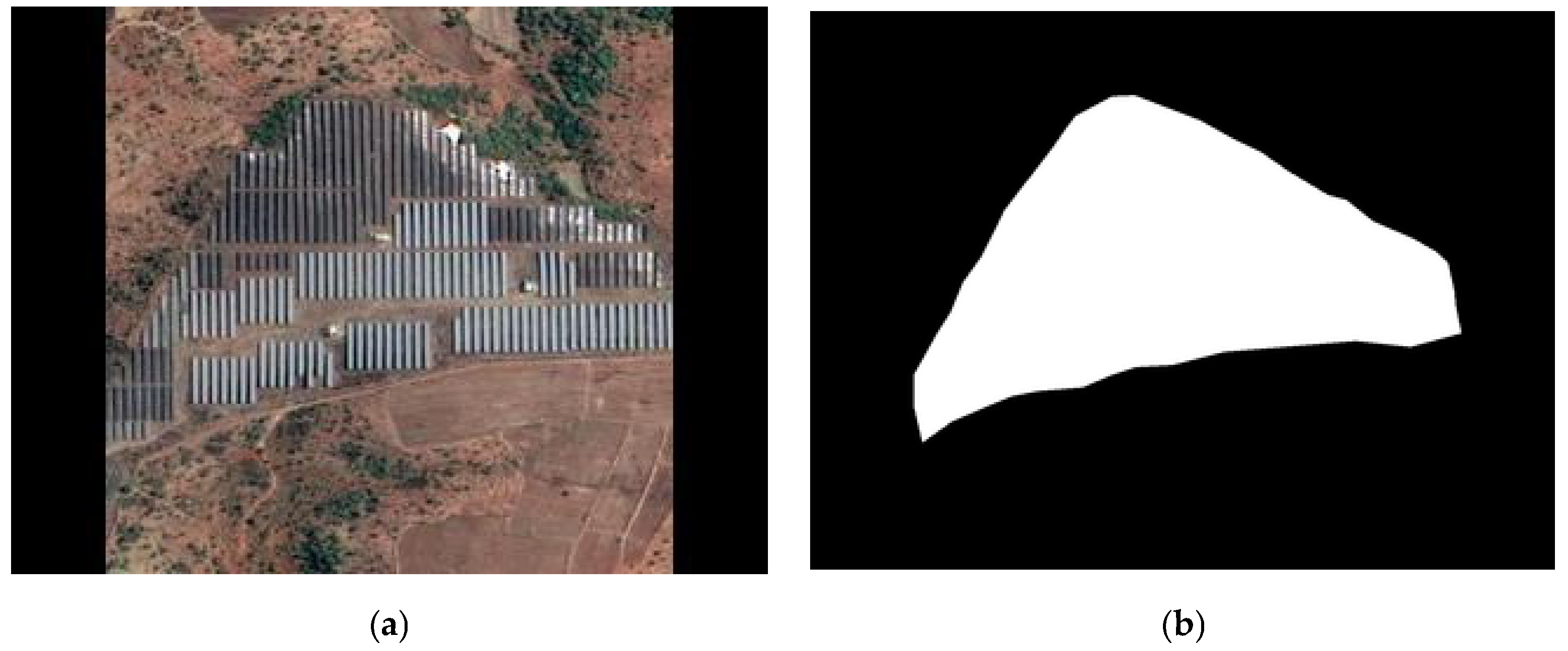
Figure 1a shows a sample aerial image in the dataset, and Figure 1b shows the corresponding mask for the sample image. If we can generate the mask as shown in Figure 1b, we can successfully detect the boundary for the solar plant.
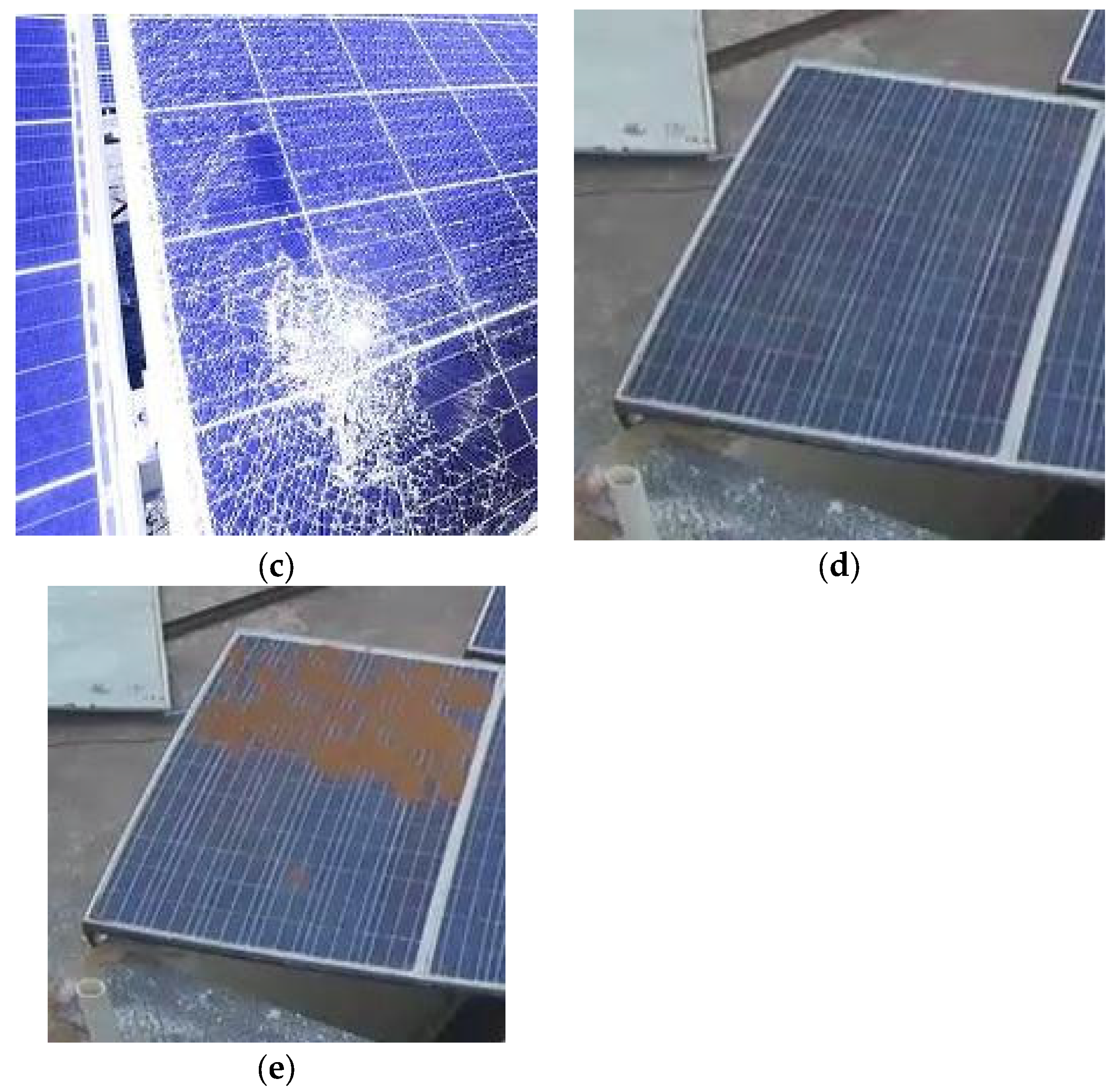
Figure 2a–e below depict the various types of solar panel impairments which happen frequently. Though cracks are a form of permanent damage and require a lot more effort to repair, for the sake of damage classification, we assigned equal importance to all the types of classes. When implemented as a real-world application, based on the type of damage identified, the level of warning generated can be programmed to match the severity of the damage. Overall, around 200 images of each type of damage were collected, mostly sourced from [22] and other solar panel damage repair and cleaning organizations. The images were then augmented to prevent under-fitting. As a result, 560 images were obtained for each type of damage, resulting in a dataset of 2800 images. The dimensions of the image were 224 pixels in width and 224 pixels in height. Since most of the models are trained for dimensions around this size, these dimensions were chosen. The augmentation of the images is explained in the next section.

2.2. Data Preprocessing

The dataset of Amir [3] is already preprocessed. Thus, we used the data directly without any additional processing. In cases of damage classification, since the dataset contained only 1000 images, augmentation was required to prevent under-sampling and over-fitting. The main augmentations performed were horizontal flipping and rotations with random angles. This task was performed using the cv2 library in the Python environment. The dataset was first split into training and testing datasets, with the test dataset containing around 50 images per class. The training data were then augmented using rotations with random angles and horizontal and vertical flipping to generate an augmented dataset. This augmented dataset, consisting of around 2500 images, was used for training the models.

2.3. Segmentation

In a number of research areas, such as computer vision, medical imaging, and natural language processing, segmentation models are gaining popularity. These models are designed to locate and separate particular areas of interest in an image or text. Convolutional neural networks (CNNs) and recurrent neural networks (RNNs), two deep learning techniques, have recently demonstrated great promise for producing accurate and effective segmentation results. In the proposed approach, we will investigate the use of a deep learning-based segmentation model to separate and examine solar plant images for boundary detection.

2.3.1. UNet

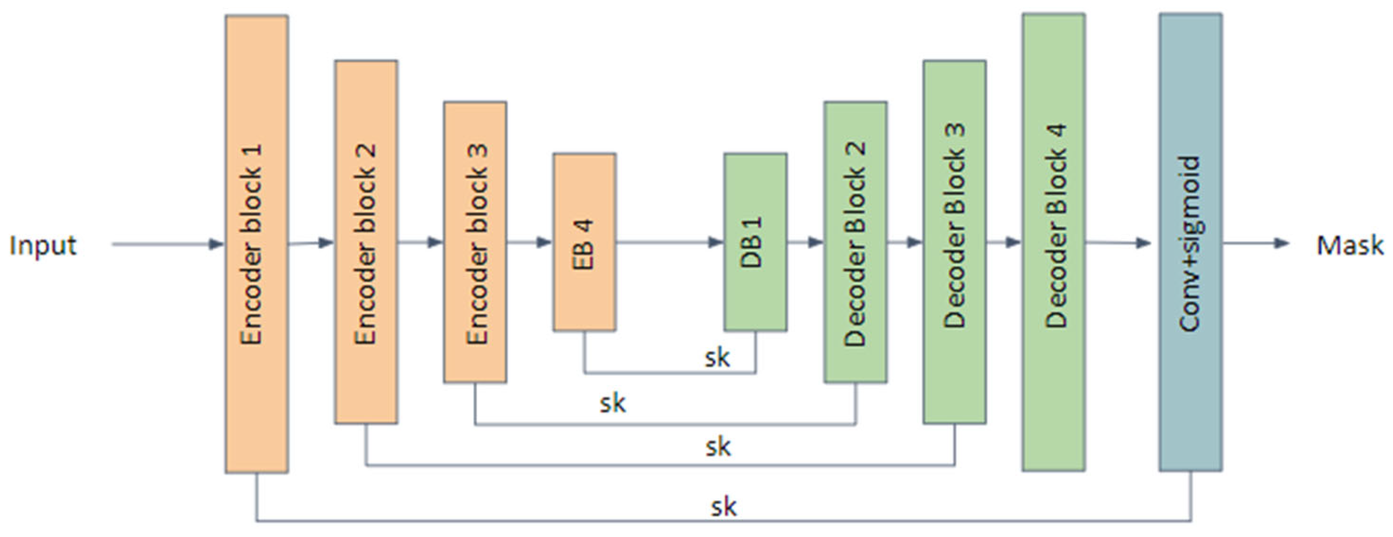
In a number of research areas, UNet [23] is a well-known segmentation model in the domain of medical image segmentation. The UNet model is based on the architecture of an encoder–decoder model. In this architecture, the input is passed through an encoder whose function is to compress the features and also extract feature information from the input. The compressed feature output is then passed to a decoder, which performs image upsampling and transpose convolution, finally generating the original image. The main purpose of this model is to generate a low-dimensional representation of the input for further processing. In the UNet architecture, the outputs of encoder blocks are used in the encoder layers as skip connections for the decoder to scale up on. By doing so, the amount of feature information at hand for the decoder blocks is increased, thus improving their performance.
Figure 3 shows the general implementation of the UNet architecture. The depth of the architecture, which is basically the number of encoders to use, is up to the implementation. Reducing the depth of the architecture would decrease the number of parameters and the amount of computation, but would also compromise the performance of the model.
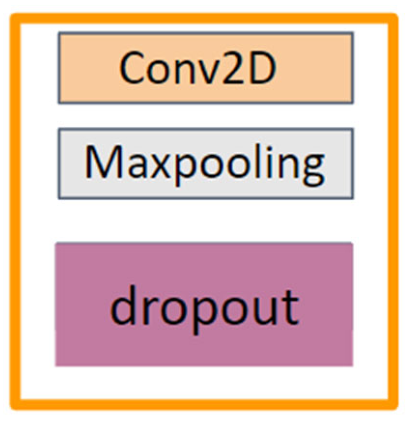
The encoder layer consists of a Conv2D block, as shown in Figure 4, followed by a max pooling block of stride size 2, followed by a dropout block. We used a dropout ratio of 0.1. The dropout layer was added to prevent the over-fitting of the model.
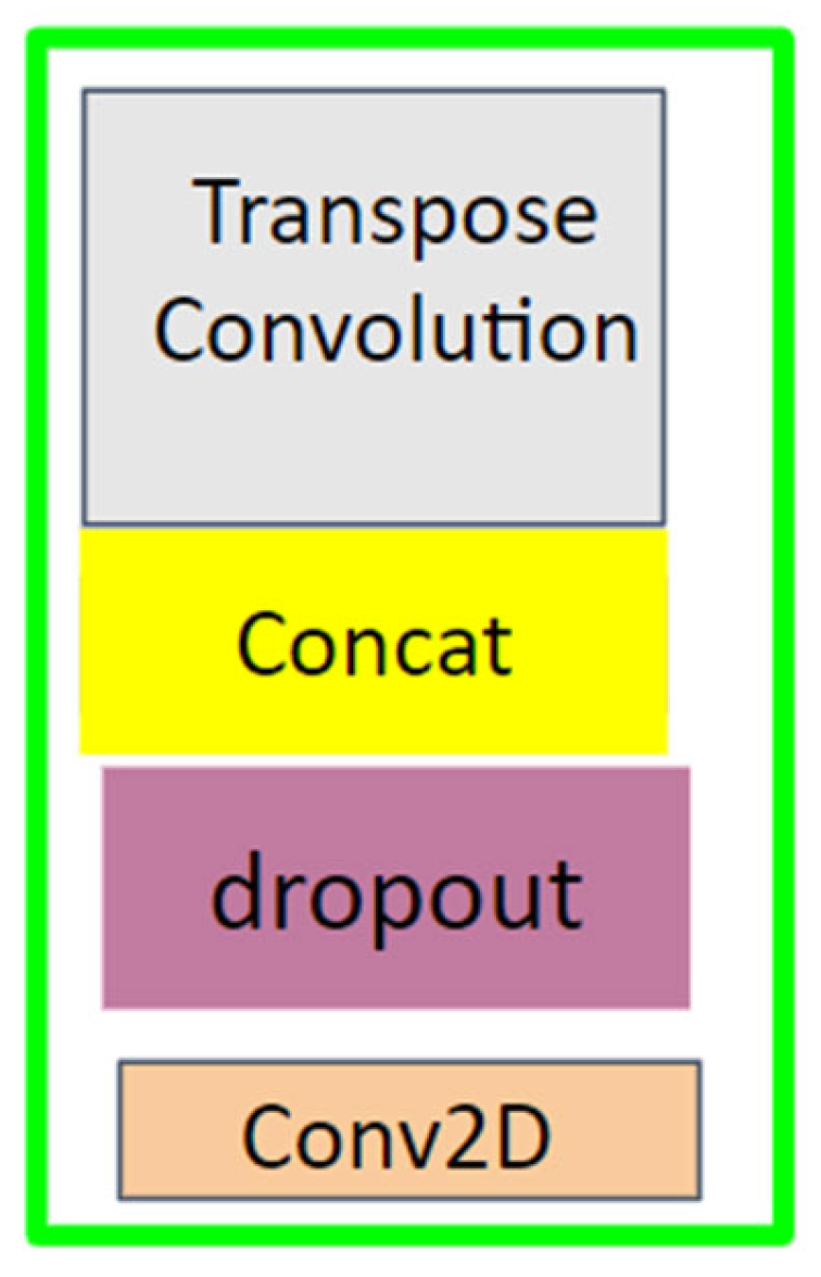
From encoder blocks 1 to 4, the number of filters in the 2D_Convolution_1 operation were doubled, and from decoder blocks 1 to 4, the number of filters were halved. For our implementation, we started with a filter count of 16, and thus for encoder 1, the number of filters was 16, and for encoder 4, the number of filters was 256. For DB1, the number of filters was 256, and for decoder block 4, the number of filters was 16. The output of the Conv2D block for each encoder block was taken as the skip connection and used in the concatenation operation of the decoder block. Skip connections help to provide fine-grain details which assist making better predictions; apart from this, they also reduce the problem of vanishing gradients. Unlike Resnet [24], where skip connections are added to the outputs, in UNet, skip connections are concatenated with the input and feed into the model. The skip connections are also established in a symmetric manner; the encoder and decoder connected by the skip connections have the same number of filters. For the upscaling of images, instead of directly upscaling the image and performing the convolution operation, we used a transpose convolution with a kernel size of 3 × 3 and a stride size of 2 with the filter count based on the position of the decoder block in the architecture. The output of the last decoder block was passed through a 2D_Convolution layer with a kernel size of 1 × 1 and sigmoid activation to predict the class of each pixel, as shown in Figure 5. Table 1 shows the architecture of the 2D Convolution Block with the appropriate involved layers.

2.3.2. AUNet with ASPP

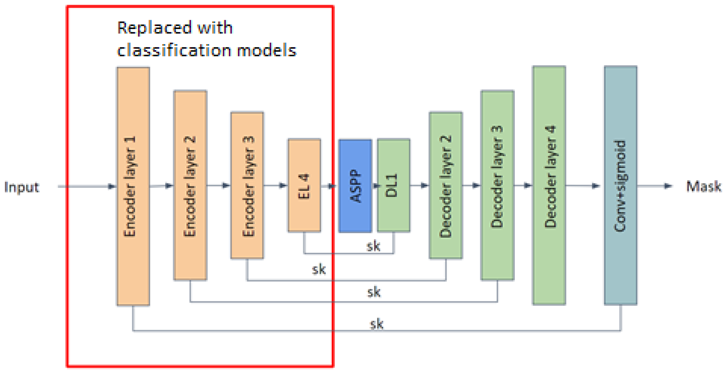
To increase the performance of the UNet model while still requiring almost the same number of computations, we modified the UNet module with the addition of an attention mechanism using dilated convolutions and designed a model called AUNet (Adaptive UNet). The encoder and decoder architectures are similar to the UNet model, as shown in Figure 6, but additionally the final output of the block is passed through a squeeze-and-excite network [25]. At the bottleneck of the model, we added an ASPP [26] module between EB4 and DB1.
We also created a variation of this architecture by replacing the entire encoder module with VGG19 [27] as the backbone. The VGG19 backbone is used for feature extraction, and since even in VGG the feature map size is gradually reduced to represent the input in a lower dimension, this is feasible. In the decoder block, instead of using a transpose convolution, we used bilinear upsampling to reduce the model complexity. The same filter count as the UNet model was used here. The block1_conv2, block2_conv2, block3_conv4, and block4_conv4 outputs were used as skip connections for the corresponding decoder blocks. Unlike AUNet, this implementation is not symmetric because the number of layers in the encoder network is more than that of the decoder network.
The loss function used for the training of the segmentation models was the dice loss function given in Equation (1). It is calculated as the dice coefficient given in Equation (2) subtracted from Equation (1):
d i c e   l o s s = 1 d i c e   c o e f f i c i e n t
Since in our task we have two classes, the solar panel and the background, and in most of the images the background occupies most of the pixel area, we can say that we have a class imbalance in terms of background to object classes. Thus, rather than using cross entropy, it is wise to use dice loss, since it gives a penalty for false negative and false positive predictions equally.
d i c e   c o e f f i c i e n t = 2   X Y X + Y  
We used Adam [28] with a learning rate of 0.0001 as the optimizer for training the segmentation models. Adam has the benefits of both gradient descent and momentum, which makes the learning rate adaptive, and thus the model converges at a faster rate and avoids the problem of becoming stuck at local minima. Not only does it increase the accuracy of the model, it also reduces the training time, and thus we used Adam as an optimizer.
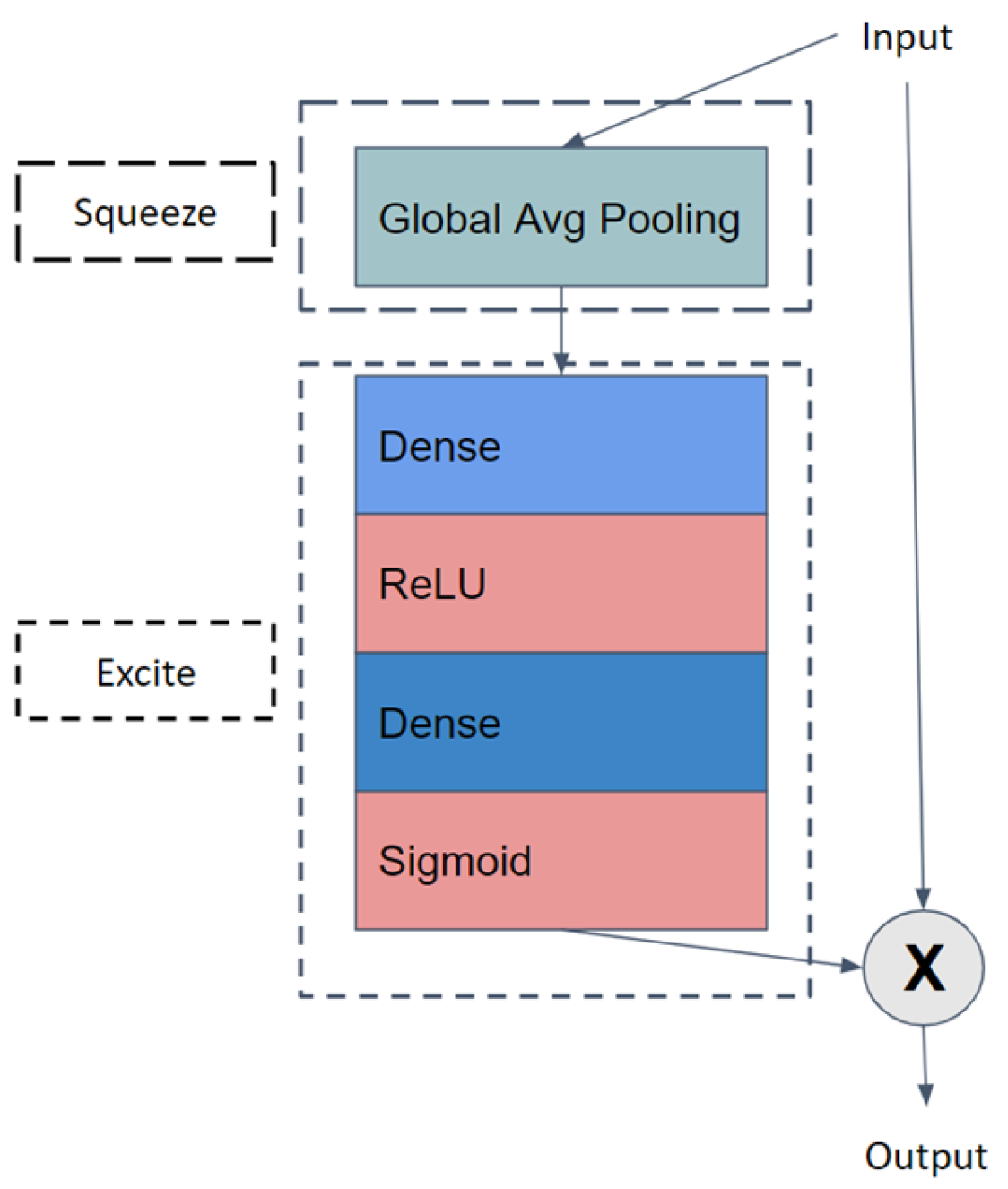
The “Squeeze and Excite” (SE) block is a neural network module shown in Figure 7 that can be used to improve the accuracy and efficiency of a segmentation model. The SE block compresses the feature maps from a convolution layer into a smaller number of channels and then uses these channels to weight the importance of each channel in the original feature maps. This helps the network to concentrate on the most informative features, resulting in a more accurate and efficient model.
By performing a Global Average Pooling operation, we reduced the dimension of the inputs to (1, 1, C), where C is the number of channels in the input. This squeezes the input; following this, we performed the excite operation, where the first dense operation uses C/8 neurons. The second dense layer has c neurons, thus producing an output with a shape of (1, 1, C). The activation for the second dense layer is sigmoid; this is used so that each of the C channels’ output is a value in the range 0 to 1, representing the importance of the channel. The channel attention produced by this network is multiplied with the input to this network and given as an output.
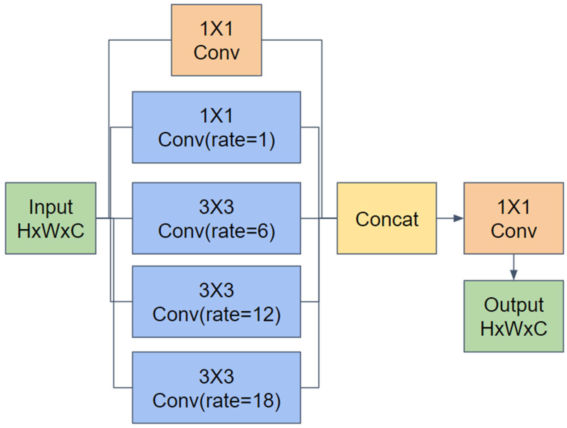
The ASPP module is a segmentation technique that resamples the feature layer at multiple rates. This applies dilated convolutions with multiple fields of view by using different dilation rates. This helps to encode the feature information from multiple fields of views into channels for the next blocks.
ASPP operates on the input image by applying a series of filters with varying dilation rates. The dilation rate determines the spacing between filter elements, allowing the network to capture features at various scales. As a result of examining the image at various scales, ASPP is able to gather both small-scale details and more comprehensive contextual data.
The architecture of the ASPP network was as shown in Figure 8. As a useful method for image segmentation, ASPP possesses a number of significant characteristics. First, it has the ability to capture both global and local image features. This indicates that the network can precisely segment foreground objects while also taking the surrounding context into account. Second, ASPP is computationally effective and is simple to incorporate into the architectures of other models which slightly increase the number of parameters.

2.4. Classification

The second problem we worked on is the classification of damage on the solar panels. The main use of this would be in creating a system which analyzes the videos captured by either CC cameras or UAVs and identifies any damage done to the solar panel and reports to the monitoring dashboard. If the UAV records geographical information, we can also show the location of damaged solar panels on the map. For the task of classification, we chose a transfer learning approach. The major advantage of transfer learning is that the weights of the model are obtained by training large datasets such as ImageNet [29]. Thus, transfer learning models have kernels trained which effectively capture various spatial and color patterns in the image required for the classification of the image. The next sections will discuss the models used for transfer learning.
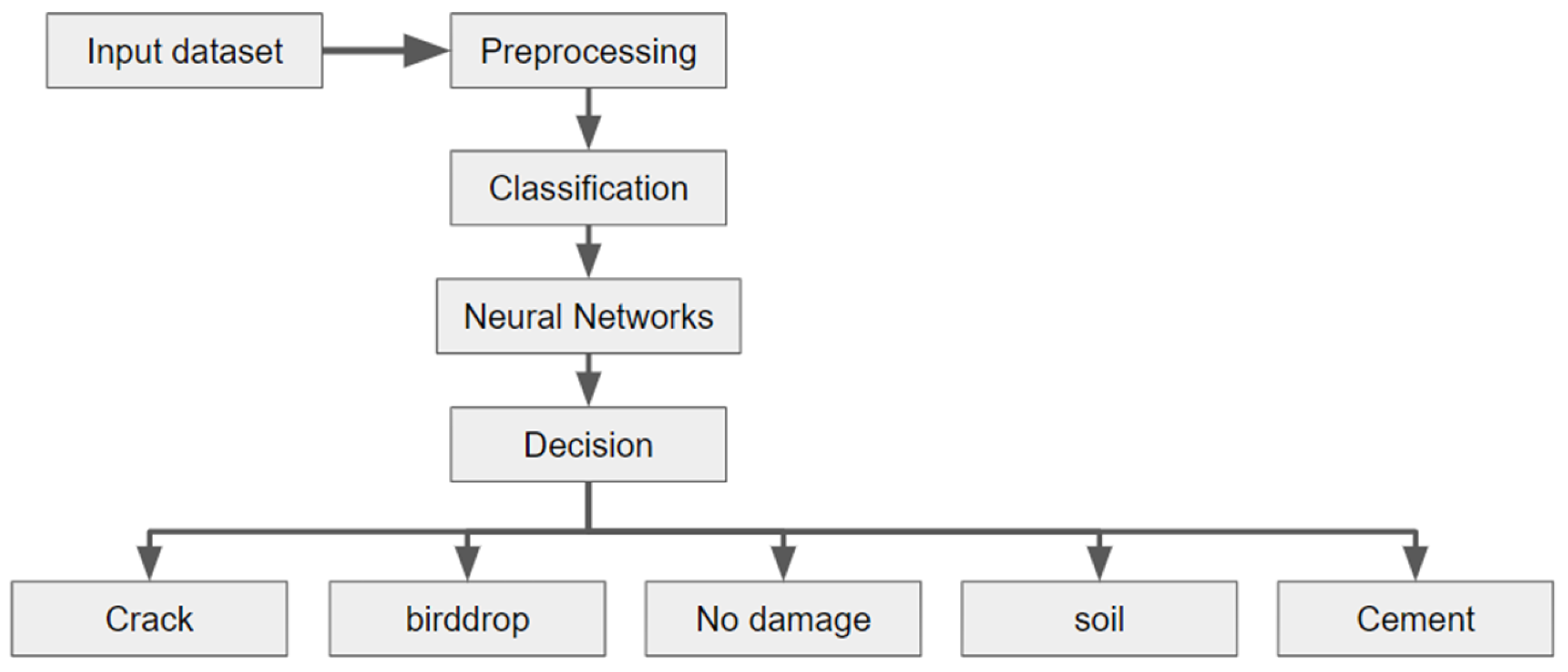
Figure 9 depicts the methodology of classification that we followed. After the preprocessing of the data, the classification was performed using a neural network model. The decision of the model was converted into one of the four types of damage or the no damage category. The no damage category was used to detect if the solar panel was clean, useful in applications where a recorded alert instance is made only if the category is something other than the no damage category. Figure 10 gives the architecture of the classification model with the suitable blocks that help for classification. Layer-wise architecture details for the classification architecture shown in Figure 10 are listed in Table 2.
The above chart shows the generic architecture followed for the classification of solar panel damage. The next five sections explain the various classification models used as the backbones for the classification model’s feature extraction. Based on the features extracted from the backbone, few dense layers are added to make the predictions.
In Table 2, ? refers to the batch size used for training. C represents the number of channels returned by the backbone model. If we consider the output dimension of the backbone to be (?, H, W, C), where H is the height of the feature and W is the width of the feature, applying Global Average Pooling would take an average of all the HxW features points in each of the C channels and result in an output with the shape (?, C). Dropout, introduced in [30], is a method used to prevent over-fitting in neural networks. Dropout was included to prevent the over-fitting of the model; by default, for each model next used as the backbone, we used a dropout rate of 0.3, and if a different rate was used, it is specified in the models section. A dropout rate of 0.3 means that 30 percent of the output generated by that layer is zero and the output selection is performed randomly. For the layers dense_5 and dense_6, we used L2 kernel regularization. L2 kernel regularization is another technique to reduce over-fitting. In L2 regularization, the loss function of the model is slightly modified by adding an L2 regularization term to it. In L2 regularization, the Euclidean norm of the weight matrix is taken and multiplied with a scalar constant and divided by 2; this term is added to the loss function. This addition of the regularization term to the loss function is also reflected in the gradient calculations.
The loss function used for the implementation of the classification model was categorical cross entropy.
C E = i C t i   ×   l o g   l o g   s i        
The calculation of cross entropy, as given in Equation (3), was performed as a summation of each class, wherein t i represents the ground truth, which is one for the true class and zero for other classes; and s i is the prediction made by the model. In our case, it is the result of the softmax function applied to the outputs of the dense-7 layer. The optimizer used for the training of the model was Adam with a learning rate of 0.0001. The implementation of these classification models was performed in a Google Colab environment and all these models were trained for 30 epochs on a GPU.

2.4.1. VGG19

Visual Geometry Group (VGG) [27] is a CNN architecture for image classification. The main novelty of VGG is that it contains small 3 × 3 convolution filters that provide more information in terms of the patterns it recognizes. In our implementation, we used VGG19, which is a 19-layered model. The output size of the VGG19 model is (?, 7, 7, 512). The main reason to use VGG19 is that it outperformed state-of-the-art models in ImageNet classification, and thus using VGG19 for feature extraction would make the task of identifying important features and patterns for classification much easier.

2.4.2. MobileNet

An architecture for convolution neural networks called MobileNet [31] was created especially for mobile and embedded devices. Its use of depth-wise separable convolutions, which drastically decrease the number of parameters and computations needed to be compared to typical convolutions, gives it a distinct advantage and makes it the best choice for low-power devices. A depth-wise convolution layer, which applies a different filter to each input channel, replaces the standard convolution layer in this method. This stage is followed by a point-wise convolution layer, which employs a 1 × 1 filter to merge the outputs of the previous layer. When this is achieved, fewer computations are required while maintaining an excellent level of accuracy. The final result of MobileNet in our instance had a size of (?, 7, 7, 1280).

2.4.3. InceptionV3

The InceptionV3 [32] convolutional neural network architecture was developed to achieve superior accuracy in image classification while utilizing the fewest possible parameters and computations. The capacity of it to collect features at various scales is made feasible by the use of inception modules, which are made up of several parallel convolution layers with different sizes of filters and pooling procedures. In our implementation, InceptionV3’s output shape was (?, 5, 5, 2048). With this approach, the network’s depth and width were increased while the computational cost was kept reasonably low.

2.4.4. ResNet50

The issue of vanishing gradients in very deep neural networks was the inspiration for the creation of the ResNet50 [24] convolution neural network architecture. The incorporation of residual connections, which allow knowledge obtained from earlier layers to pass through later layers and make it simpler to train very deep networks, provides it its uniqueness. ResNet50 works at the cutting edge on an array of image recognition tasks, including the ImageNet Large Scale Visual Recognition Challenge. It comprises 50 convolution layers, including convolution layers, pooling layers, and fully connected layers. ResNet50’s residual connections help to solve the vanishing gradients issue, enabling it to train very advanced neural networks. Without these connections, as the gradients spread through the network, they become progressively smaller, making it difficult to train deep networks. ResNet50 makes sure that the gradients are large enough to train the network effectively by allowing data from earlier layers to skip over later layers.

2.4.5. EfficientNet

The most compact component of the EfficientNet family, EfficientNetB0 [33], was designed to achieve outstanding performance on image recognition tasks with a minimal number of parameters and computation required. The application of compound scaling, which combines scaling the network’s depth, width, and resolution in a principled manner to produce a highly effective architecture, gives it a unique edge over other systems.
Various components, such as convolution layers, pooling layers, and fully connected layers, make up EfficientNetB0. Nine MBConv layers, or mobile inverted bottleneck convolution layers, make up its 19-layer architecture. The final convolution layer’s output shape is (batch_size, 1280, 7, 7), where 1280 is the output channel count and 7 × 7 is the feature map’s spatial resolution.

3. Experimental Results and Discussion

3.1. Performance Metrics

The metrics used for evaluating the performance of various models that we used for the task of damage classification were accuracy, precision, recall and F1 score. Accuracy is the ratio between the number of predictions that are correctly made and the total number of predictions made. Precision and recall are metrics based on relevance. Precision can be defined as the fraction of true predictions as shown in Equation (4), which match with the ground truth out of all the predictions made. Since the task is classification into multiple classes, the definitions of TP, FP, TN, and FN are slightly different in terms of their calculations. The calculations are represented in terms of the confusion matrix.
P r e c i s i o n = T P T P + F P
where TP (true positive) is the number of predictions where the actual class and predicted class match; FP (false positive) is the number of predictions where the predicted class is not the same as the actual class, i.e., it is the sum of values of a corresponding column except for TP values; FN (false negative) is the sum of the values of rows except for the TP values; and TN (true negative) is the sum of values of all columns and rows except for the values of the class that the values are being calculating for.
Using the above defined calculations, we can define recall as shown in Equation (5).
R e c a l l = T P T P + F N
High precision and recall are good indications of an efficient model. Giving equal importance to both precision and recall, since in our case making correct predictions was equally valued with not making wrong predictions, we also used the F1 score, shown in Equation (6), which is twice the harmonic mean between precision and recall, as another metric for evaluating the performance of the model.
F 1 S c o r e = 2     P r e c i s o n     R e c a l l P r e c i s i o n + R e c a l l
Other than this, to evaluate the training performance of the model, we monitored the trends in the training loss, accuracy, and validation loss and looked at how the model performed on the validation dataset. The fit of the model was evaluated based on the performance shown while using the training dataset.

3.2. Classification Results

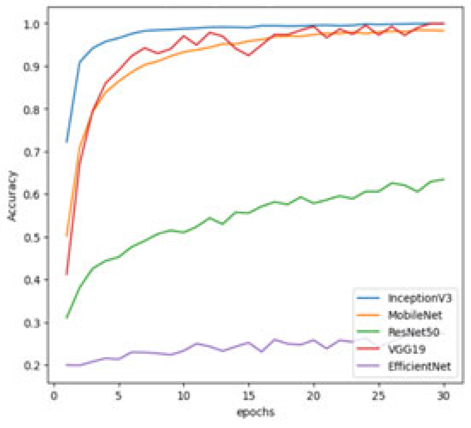
From Figure 11, one can understand that in the first five epochs, the loss of the VGG19 model was very high in comparison with the other models, but by the end of 30 epochs, the losses of VGG19, InceptionV3, and MobileNet stabilized and reached close to zero, indicating that they reached the point of best fit for the given model. Even the training accuracies of the three models, as shown in Figure 12, were high at the end of 30 epochs. But one can entirely rely on the training accuracy of the models to evaluate the models, and thus we also looked at the validation performance of the models. One trend that is observed is that the EfficientNet loss is almost the same in the entire process of training, with a slight improvement in terms of accuracy; this is an indication that the EfficientNet model was under-fitted for the given data.
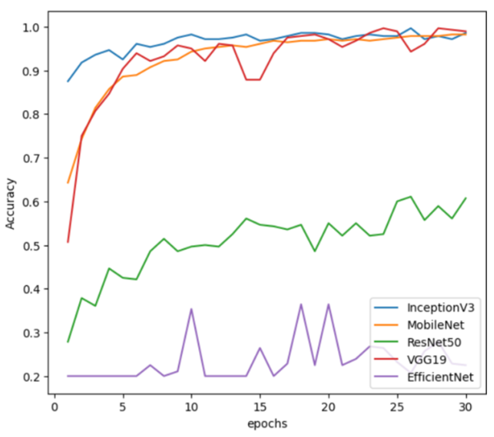
From Figure 13 and Figure 14, we can observe similar trends in terms of the validation loss and accuracy of various models. For VGG19, InceptionV3, and MobileNet, we can observe that even with validation data, they performed very well in terms of accuracy. Based on the validation loss, which smoothly decreased to zero by the end of thirty epochs, we can say that all the three aforementioned models fitted very well on the training data and performed well on the validation data. Thus, no case of over-fitting was observed. Since there are no class imbalances in the dataset, we expect the precision and recall of the models to match with the F1 score.
Since this is a task involving multiclass classification, in the calculations of precision, recall and F1 scores, the metrics were calculated individually of each class and their mean is represented in Table 3. VGG19 has the highest accuracy (98.6%) and F1 score (99%), indicating that it performs the best overall among the five models. VGG19 also has the highest precision and recall, both at 99%. MobileNet and InceptionV3 also have high accuracy and F1 scores, but are slightly less accurate than VGG19.
On the other hand, ResNet50 and EfficientNetB0 have significantly lower accuracy and F1 scores. ResNet50 has a precision of 65% and a recall of 64%, while EfficientNetB0 has a precision of 13% and a recall of 23%. These lower values indicate that these models are not performing as well as the other three models when correctly classifying the images in the test set. Overall, in comparison, the VGG19 model outperformed the other models with an overall accuracy of 98.6%. As expected, the EfficientNetB0 model performed poorly, with an accuracy of 23%. In terms of F1 score, the VGG19 model obtained a mean F1 score of 99%, not only outperforming the other models, but also outperforming models discussed in the literature. Thus, we created a highly accurate model for identifying the types of damage done to solar panels.
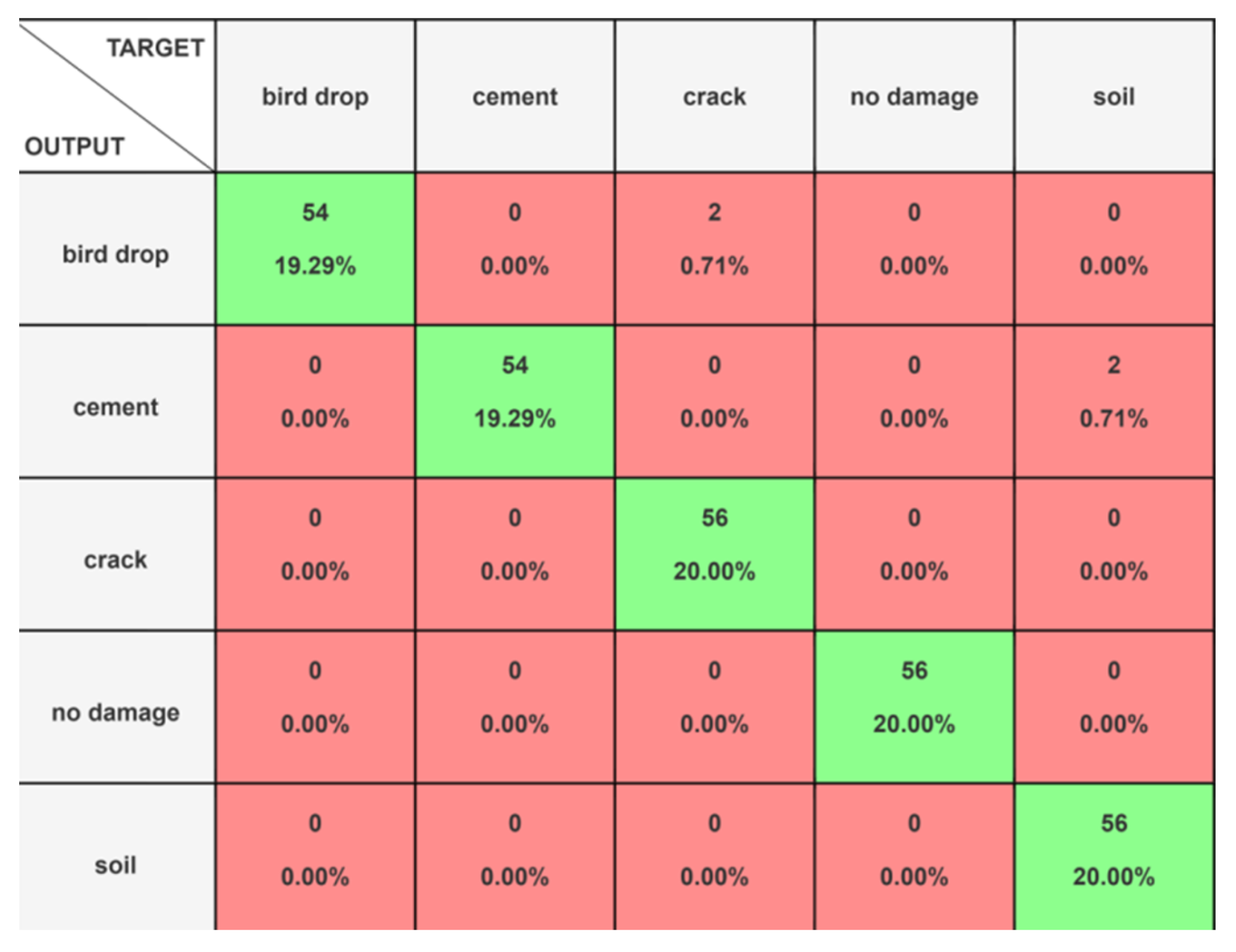
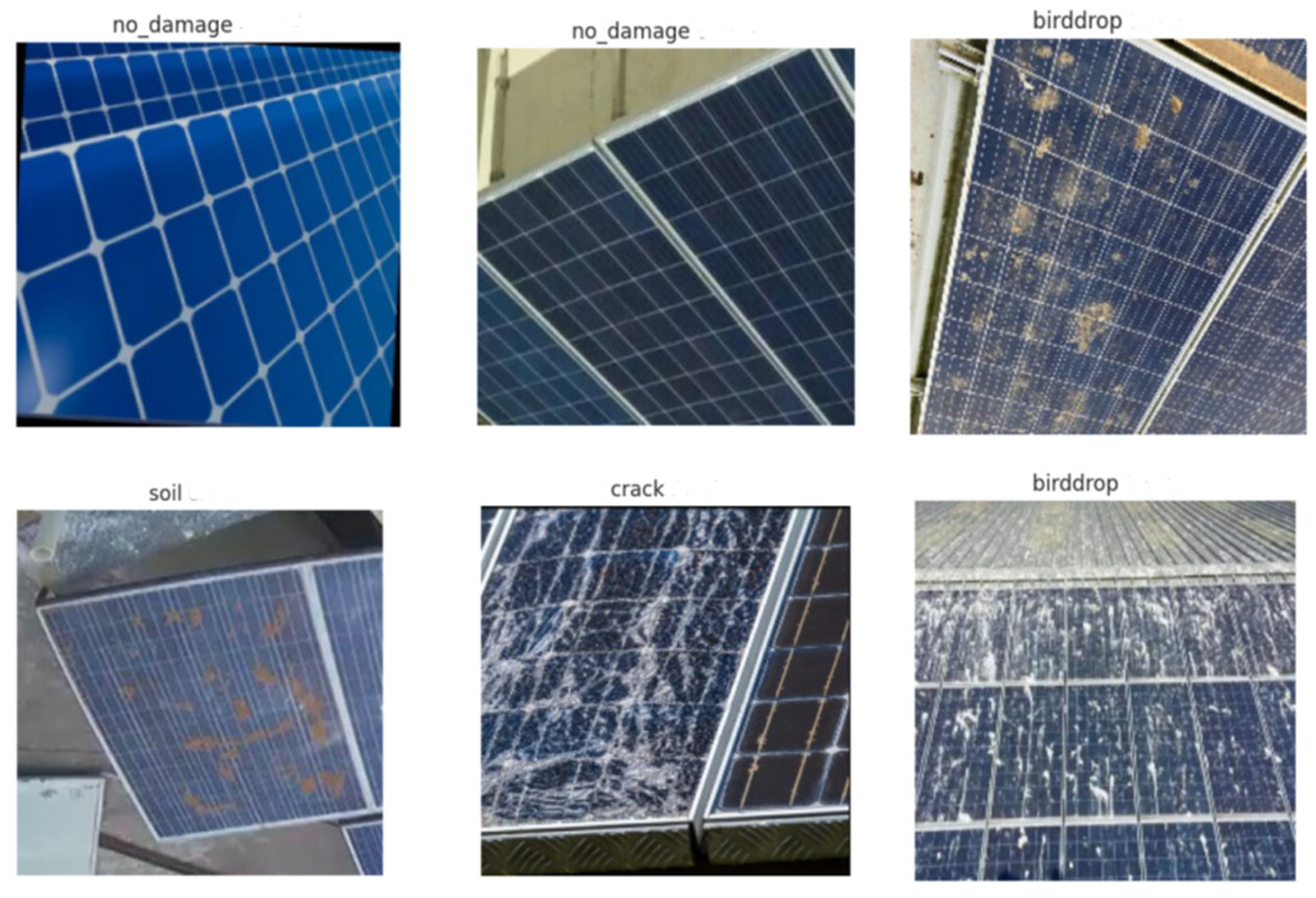
From Figure 15, we can see that except for bird droppings and cement damage, for all the other classes in the testing data, there was no misclassification. Figure 16 contains a few sample predictions made by the VGG19 model.

3.3. Segmentation Metrics

A higher mean IOU score in the context of picture segmentation suggests better segmentation accuracy because it measures the amount of overlap between the anticipated and actual masks. When measuring the efficacy of models that create segmentation masks, where the distinctions between object classes are not clearly defined, this metric is very helpful.
I o U = T P T P + F P + F N
MeanIoU is the summation of IoU shown in Equation (7) for all images in the corresponding dataset. The performance of image segmentation models is frequently assessed using the Mean Intersection-over-Union (IOU) measure. IOU estimates the ratio of the intersection of the two masks to their union by measuring the overlap between the predicted segmentation mask and the ground truth mask for each pixel in the picture. The average of the IOU ratings for each pixel in the image is then used to determine the mean IOU.
It should be mentioned that mean IOU has limitations despite being a statistic that is frequently employed in picture segmentation studies. For instance, it does not consider the degree of segmentation error in each particular object class or the geographic distribution of defects inside the segmentation mask. To obtain a more thorough insight into model performance, researchers might also think about employing other indicators, like pixel accuracy.
Apart from mean IoU, we also used pixel accuracy and F1 score as metrics. F1 score is calculated individually for each image, which is divided into two classes: one is the background and other is the mask area. Neural networks are an excellent choice for a lot of image processing problems, but the major drawback they have is the consumption of resources and the high computational requirements needed to process the image and make a prediction. When creating models that may be deployed in real-world systems such as UAVs, automobiles, and CC cameras, a major concern is the amount of time they take to process the image, and thus we also added processing time as a metric for evaluating the model. Based on the use case requirements and resources at hand, corresponding implementations can be used. We defined processing time as the time taken in seconds from the moment the input is provided to the model to the moment the mask is generated by the model. In our experiments, we measured it in seconds.

3.4. Segmentation Results

To compare our model’s performance, we also trained UNet and DoubleUNet [34] along with our proposed model. UNet was used as a reference since we used a modified version of UNet. We used DoubleUNet because this model has outperformed UNet in medical segmentation and has also been used for segmentation in other domains, showing great efficiency on a large number of datasets.
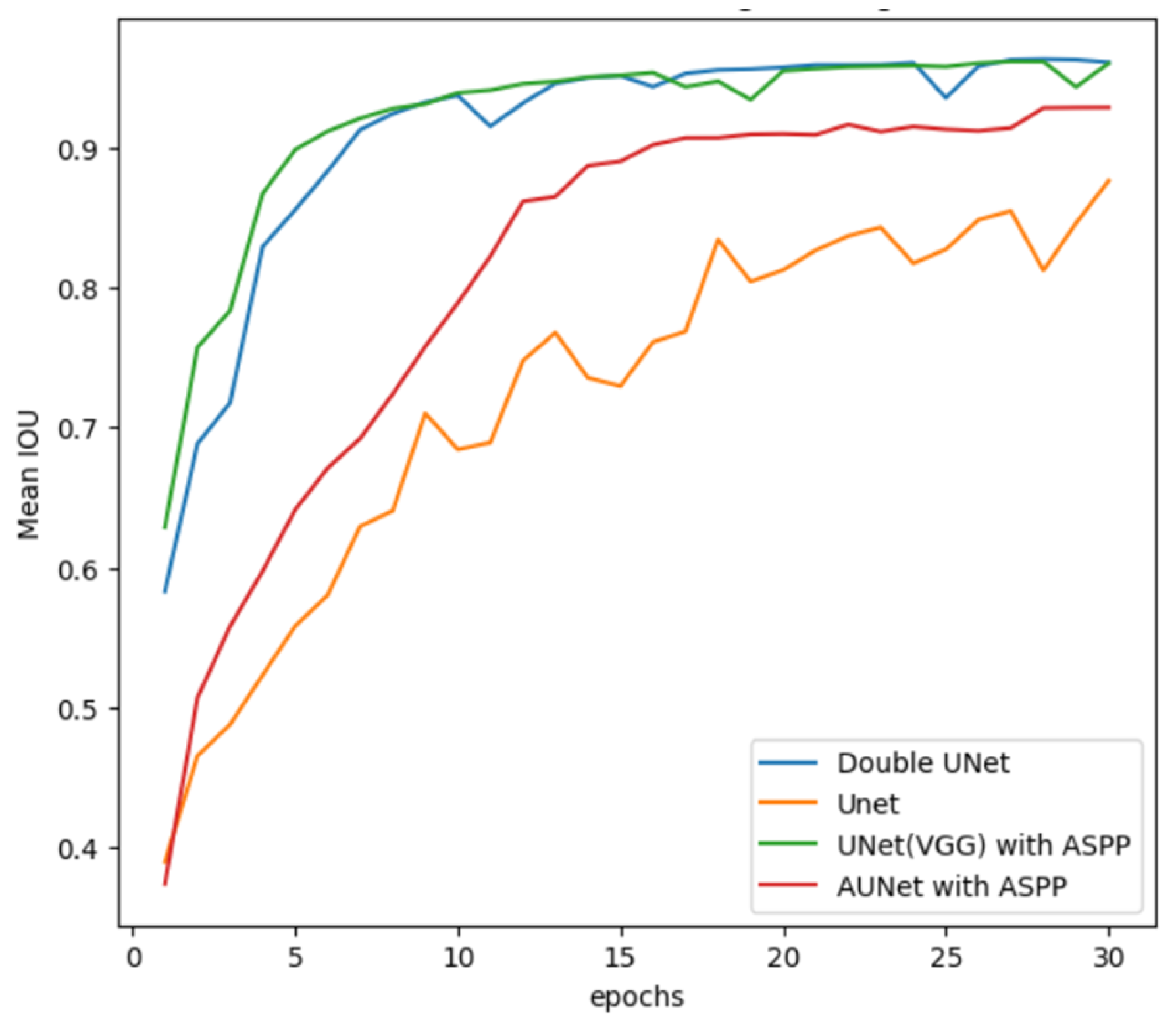
Figure 17 shows that in the 15 epochs, the training loss of the segmentation model was very high in comparison with the other models, but by the end of 30 epochs, the loss of all models approached zero, indicating that they reached the point of best fit for the given model. Even the training mean IoUs of the models were high at the end of 30 epochs. UNet had a lower training mean IoU in comparison with other models, and even its loss was a bit high in comparison with other models, but considering the smooth decrease in loss during the training we can say it attained its best fit. Though AUNet started with a low mean IoU, at the end of training, its mean IoU performance was close to the UNet (VGG) and DoubleUNet models. Figure 18 depicts the training mean IoU plot of segmentation models.
In terms of validation loss, from Figure 19, we can observe that among all the models, AUNet has the smoothest curve in terms of loss and mean IoU as shown in Figure 20 based on validation data. Based on the performance of the models on the validation data, we expect the AUNet model with the VGG backbone to outperform other models. Also, though some models still reached the best fit given their limitations, none of them over-fitted nor under-fitted, which is a good indication. The comparison of the models used for segmentation is listed in Table 4, where pixel accuracy, mean IoU, F1 score, processing time and the number of parameters used are compared.
Due to the large number of parameters present in the segmentation models, the processing time the model takes for an image increases, and it requires more time and resources for training and maintenance. Our aim was to create a model with low processing time and with less parameters in comparison to the literature. By analyzing the results, we understand that in terms of overall performance, AdaptiveUNet showed better accuracy (98%) and mean IOU (95%). It was able to process an image in under one second with 23 times fewer parameters than the DoubleUNet or AUNet models with a VGG backbone.
Apart from the inclusion of the VGG model as a backbone, no major changes were made to the model, but since VGG is a 19-layer model with lots of parameters, its total parameter count reached that of DoubleUNet, a model with two UNet networks in it. If we compare the performance of AUNet with UNet, we increased the accuracy by three points and the Mean IoU score by three points. The processing time increased by only 0.1 s and the number of parameters increased by only 0.27 million. Thus, for large segmentation networks, we can say that the addition of an attention mechanism and ASPP module comes with a small cost in terms of the number of parameters, but also shows a gain in performance. If the use case requirements are high performance, then we can use the AUnet model with a VGG backbone. In comparison with DoubleUNet, it has a slightly better performance in terms of accuracy, Mean IoU, and F1 score and it has almost half the process time per image as that of DoubleUNet.
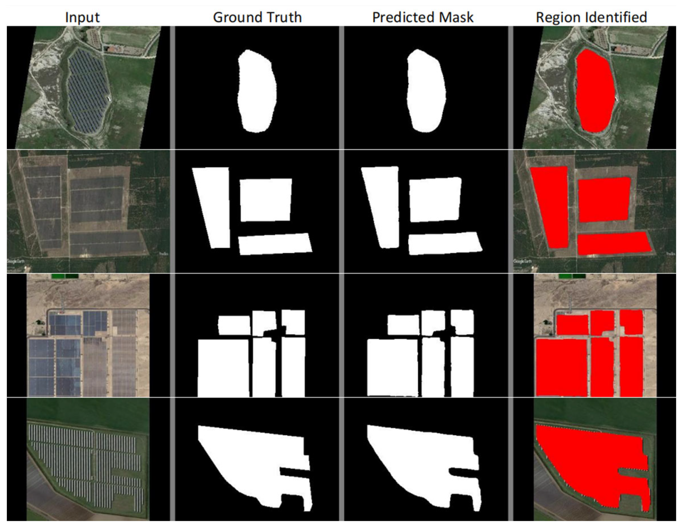
Figure 21 shows some predictions made by the AUNet model without the VGG backbone. The last column (Region Identified) was generated using the Predicted Mask. By superposing the Predicted Mask onto the original image and assigning it a red color, we obtained the last column. If we have the scale information of the aerial image, i.e., the proportion between the number of pixels and the length on the surface, we can compute the approximate area of each solar plant. The proportion information may be obtained by taking into consideration the height of the UAV or the camera specifications, or can be manually calculated.
4. Conclusions and Future Work

The segmentation of solar power plant aerial images has many associated use cases. These can be applied to Coverage Path Planning so that autonomous UAV plant monitoring is possible. They can be used to estimate the approximate area of solar plants. They are also able to extract the solar panels from an image which can be used for other processing purposes. In this article, we proposed a deep learning model for the segmentation of solar power plants which is efficient in processing the images in less time and has a low memory profile in terms of the number of parameters. The performance of the model in terms of accuracy and Mean IoU is very high (98% pixel accuracy and 95% Mean IoU). The second major work carried out in this paper is the classification of solar panel damage. We classified the damage into a total of five classes, with one of the classes being no damage. Overall, we have outperformed the models listed in [18,19] with an accuracy of 98% and an F1 score of 99% utilizing the transfer learning approach with VGG19 as the backbone.

Author Contributions

Conceptualization, A.S. and A.B.; methodology, A.S.; software, A.S. and L.S.K.; validation, A.S., A.B. and N.M.; formal analysis, A.S., A.B., L.S.K. and N.M.; investigation, A.S. and A.B.; resources, A.S.; data curation, A.S.; writing—original draft preparation, A.S., A.B., L.S.K. and N.M.; writing—review and editing, A.S., A.B. and L.S.K.; visualization, A.S., A.B. and L.S.K.; supervision, A.S. All authors have read and agreed to the published version of the manuscript.

Funding

This research received no external funding.

Data Availability Statement

Data will be shared on request.

Acknowledgments

The authors wish to thank VIT, Chennai management for motivating them to pursue this work.

Conflicts of Interest

The authors declare no conflicts of interest.

References

  1. Pérez-González, A.; Jaramillo-Duque, Á.; Cano-Quintero, J.B. Automatic Boundary Extraction for Photovoltaic Plants Using the Deep Learning U-Net Model. Appl. Sci. 2021, 11, 6524. [Google Scholar] [CrossRef]
  2. Xu, Z.; Shen, Y.; Zhang, K.; Wei, H. A Segmentation Method for PV Modules in Infrared Thermography Images. In Proceedings of the 13th IEEE PES Asia Pacific Power Energy Engineering Conference (APPEEC), Trivandrum, India, 21–23 November 2021; pp. 1–5. [Google Scholar] [CrossRef]
  3. Sizkouhi, A.M.; Aghaei, M.; Esmailifar, S.M. A deep convolutional encoder-decoder architecture for autonomous fault detection of PV plants using multi-copters. Sol. Energy 2021, 223, 217–228. [Google Scholar] [CrossRef]
  4. Ying, Y.; Qi, Y.; Rong, L.; Men, H.; Joo, Y.H. Anchor Points Based Accurate Fault Locating in Large-Scale Photovoltaic Plants via Aerial Infrared Videos. IEEE J. Photovolt. 2022, 12, 437–443. [Google Scholar] [CrossRef]
  5. Ramirez, I.S.; Chaparro, J.R.P.; Marquez, F.P.G. Machine Learning Techniques Implemented in IoT Platform for Fault Detection in Photovoltaic Panels. In Proceedings of the International Conference on Innovation and Intelligence for Informatics, Computing, and Technologies (3ICT), Virtual, 29–30 September 2021; pp. 429–434. [Google Scholar] [CrossRef]
  6. Mellit, A.; Kalogirou, S. Artificial intelligence and internet of things to improve efficacy of diagnosis and remote sensing of solar photovoltaic systems: Challenges, recommendations and future directions. Renew. Sustain. Energy Rev. 2021, 143, 110889. [Google Scholar] [CrossRef]
  7. Skumanich, A.; Ghiassi, M. The Need for AI to Optimize Dual-Use PV Installations to Extract Maximum Value. In Proceedings of the IEEE 48th Photovoltaic Specialists Conference (PVSC), Miami, FL, USA, 20–25 June 2021; pp. 459–463. [Google Scholar] [CrossRef]
  8. Dimd, B.D.; Voller, S.; Midtgard, O.-M.; Zenebe, T.M. Ultra-Short-term Photovoltaic Output Power Forecasting using Deep Learning Algorithms. In Proceedings of the 2022 IEEE 21st Mediterranean Electrotechnical Conference (MELECON), Palermo, Italy, 14–16 June 2022; pp. 837–842. [Google Scholar] [CrossRef]
  9. Shapsough, S.; Zualkernan, I.; Dhaouadi, R. Deep Learning at the Edge for Operation and Maintenance of Large-Scale Solar Farms. In Proceedings of the International Conference on Smart Grid and Internet of Things, TaiChung, Taiwan, 19–20 November 2022; pp. 27–44. [Google Scholar] [CrossRef]
  10. Feng, C.; Liu, Y.; Zhang, J. A taxonomical review on recent artificial intelligence applications to PV integration into power grids. Int. J. Electr. Power Energy Syst. 2021, 132, 107176. [Google Scholar] [CrossRef]
  11. Sizkouhi, A.M.; Esmailifar, S.; Aghaei, M.; Karimkhani, M. RoboPV: An integrated software package for autonomous aerial monitoring of large scale PV plants. Energy Convers. Manag. 2022, 254, 115217. [Google Scholar] [CrossRef]
  12. Sizkouhi, A.M.M.; Aghaei, M.; Esmailifar, S.M.; Mohammadi, M.R.; Grimaccia, F. Automatic Boundary Extraction of Large-Scale Photovoltaic Plants Using a Fully Convolutional Network on Aerial Imagery. IEEE J. Photovolt. 2020, 10, 1061–1067. [Google Scholar] [CrossRef]
  13. Razmi, H.; Afshinfar, S. Neural network-based adaptive sliding mode control design for position and attitude control of a quadrotor UAV. Aerosp. Sci. Technol. 2019, 91, 12–27. [Google Scholar] [CrossRef]
  14. Aghaei, M.; Leva, S.; Grimaccia, F. PV Power Plant Inspection by Image Mosaicing Techniques for IR Real-Time Images. In Proceedings of the 2016 IEEE 43rd Photovoltaic Specialists Conference (PVSC), Portland, OR, USA, 5–10 June 2016; pp. 3100–3105. [Google Scholar] [CrossRef]
  15. Morando, L.; Recchiuto, C.T.; Calla, J.; Scuteri, P.; Sgorbissa, A. Thermal and Visual Tracking of Photovoltaic Plants for Autonomous UAV Inspection. Drones 2022, 6, 347. [Google Scholar] [CrossRef]
  16. Prabhakaran, S.; Uthra, R.A.; Preetharoselyn, J. Feature Extraction and Classification of Photovoltaic Panels Based on Convolutional Neural Network. Comput. Mater. Contin. 2023, 74, 1437–1455. [Google Scholar] [CrossRef]
  17. Selvaraj, T.; Rengaraj, R.; Venkatakrishnan, G.; Soundararajan, S.; Natarajan, K.; Balachandran, P.; David, P.; Selvarajan, S. Environmental Fault Diagnosis of Solar Panels Using Solar Thermal Images in Multiple Convolutional Neural Networks. Int. Trans. Electr. Energy Syst. 2022, 2022, 2872925. [Google Scholar] [CrossRef]
  18. Pathak, S.P.; Patil, D.; Patel, S. Solar panel hotspot localization and fault classification using deep learning approach. Procedia Comput. Sci. 2022, 204, 698–705. [Google Scholar] [CrossRef]
  19. Deitsch, S.; Christlein, V.; Berger, S.; Buerhop-Lutz, C.; Maier, A.; Gallwitz, F.; Riess, C. Automatic classification of defective photovoltaic module cells in electroluminescence images. Sol. Energy 2019, 185, 455–468. [Google Scholar] [CrossRef]
  20. Espinosa, A.R.; Bressan, M.; Giraldo, L.F. Failure signature classification in solar photovoltaic plants using RGB images and convolutional neural networks. Renew. Energy 2020, 162, 249–256. [Google Scholar] [CrossRef]
  21. Greco, A.; Pironti, C.; Saggese, A.; Vento, M.; Vigilante, V. A Deep Learning Based Approach for Detecting Panels in Photovoltaic Plants. In Proceedings of the APPIS 2020: 3rd International Conference on Applications of Intelligent Systems, Las Palmas de Gran Canaria, Spain, 7–12 January 2020. [Google Scholar]
  22. Mehta, S.; Azad, A.P.; Chemmengath, S.A.; Raykar, V.; Kalyanaraman, S. DeepSolarEye: Power Loss Prediction and Weakly Supervised Soiling Localization via Fully Convolutional Networks for Solar Panels. In Proceedings of the 2018 IEEE Winter Conference on Applications of Computer Vision (WACV), Lake Tahoe, NV, USA, 12–15 March 2018; pp. 333–342. [Google Scholar]
  23. Ronneberger, O.; Fischer, P.; Brox, T. U-Net: Convolutional Networks for Biomedical Image Segmentation. In Proceedings of the 18th International Conference, Munich, Germany, 5–9 October 2015. [Google Scholar]
  24. He, K.; Zhang, X.; Ren, S.; Sun, J. Deep residual learning for image recognition. In Proceedings of the IEEE Conference on Computer Vision and Pattern Recognition, Las Vegas, NV, USA, 26 June–1 July 2016; pp. 770–778. [Google Scholar]
  25. Hu, J.; Shen, L.; Sun, G. Squeeze-and-Excitation Networks. In Proceedings of the IEEE Conference on Computer Vision and Pattern Recognition (CVPR), Salt Lake City, UT, USA, 18–23 June 2018; pp. 7132–7141. [Google Scholar]
  26. Chen, L.-C.; Papandreou, G.; Kokkinos, I.; Murphy, K.; Yuille, A.L. DeepLab: Semantic Image Segmentation with Deep Convolutional Nets, Atrous Convolution, and Fully Connected CRFs. IEEE Trans. Pattern Anal. Mach. Intell. 2018, 40, 834–848. [Google Scholar] [CrossRef] [PubMed]
  27. Simonyan, K.; Zisserman, A. Very deep convolutional networks for large-scale image recognition. arXiv 2014, arXiv:1409.1556. [Google Scholar]
  28. Kingma, D.P.; Ba, J. Adam: A method for stochastic optimization. arXiv 2014, arXiv:1412.6980. [Google Scholar]
  29. Deng, J.; Dong, W.; Socher, R.; Li, L.-J.; Li, K.; Li, F.F. ImageNet: A Large-Scale Hierarchical Image Database. In Proceedings of the 2009 IEEE Conference on Computer Vision and Pattern Recognition, Miami, FL, USA, 20–25 June 2009; pp. 248–255. [Google Scholar] [CrossRef]
  30. Srivastava, N.; Hinton, G.; Krizhevsky, A.; Sutskever, I.; Salakhutdinov, R. Dropout: A Simple Way to Prevent Neural Networks from Overfitting. J. Mach. Learn. Res. 2014, 15, 1929–1958. [Google Scholar]
  31. Howard, A.G.; Zhu, M.; Chen, B.; Kalenichenko, D.; Wang, W.; Weyand, T.; Andreetto, M.; Adam, H. Mobilenets: Efficient convolutional neural networks for mobile vision applications. arXiv 2017, arXiv:1704.04861. [Google Scholar]
  32. Szegedy, C.; Vanhoucke, V.; Ioffe, S.; Shlens, J.; Wojna, Z. Rethinking the Inception Architecture for Computer Vision. In Proceedings of the IEEE Conference on Computer Vision and Pattern Recognition, Long Beach, CA, USA, 15 June–20 June 2019; pp. 6105–6114. [Google Scholar]
  33. Tan, M.; Le, Q. EfficientNet: Rethinking Model Scaling for Convolutional Neural Networks. In Proceedings of the International Conference on Machine Learning, Long Beach, CA, USA, 9–15 June 2019; pp. 6105–6114. [Google Scholar]
  34. Jha, D.; Riegler, M.A.; Johansen, D.; Halvorsen, P.; Johansen, H.D. Doubleu-net: A Deep Convolutional Neural Network for Medical Image Segmentation. In Proceedings of the 2020 IEEE 33rd International Symposium on Computer-Based Medical Systems (CBMS), Rochester, MN, USA, 28 July–30 July 2020; pp. 558–564. [Google Scholar] [CrossRef]
Figure 1. (a) Aerial image of a solar plant; (b) mask of a solar plant.
Automation 05 00009 g001
Figure 2. (a) Bird droppings on solar panels; (b) cement on solar panels; (c) cracks on solar panels; (d) solar panel with no damage; (e) soil on solar panel.
Automation 05 00009 g002aAutomation 05 00009 g002b
Figure 3. Architecture of UNet.
Automation 05 00009 g003
Figure 4. Encoder block architecture.
Automation 05 00009 g004
Figure 5. Decoder block architecture.
Automation 05 00009 g005
Figure 6. Architecture of AUNet with ASPP.
Automation 05 00009 g006
Figure 7. Squeeze and Excite network architecture.
Automation 05 00009 g007
Figure 8. Architecture of ASPP network.
Automation 05 00009 g008
Figure 9. Methodology of classification.
Automation 05 00009 g009
Figure 10. Architecture of the classification model.
Automation 05 00009 g010
Figure 11. Training losses of the InceptionV3, MobileNet, ResNet50, VGG19, and EfficientNet models.
Automation 05 00009 g011
Figure 12. Training accuracy of the InceptionV3, MobileNet, ResNet50, VGG19, and EfficientNet models.
Automation 05 00009 g012
Figure 13. Validation losses of the InceptionV3, MobileNet, ResNet50, VGG19, and EfficientNet models.
Automation 05 00009 g013
Figure 14. Validation accuracy of the InceptionV3, MobileNet, ResNet50, VGG19, and EfficientNet models.
Automation 05 00009 g014
Figure 15. Confusion matrix of VGG model.
Automation 05 00009 g015
Figure 16. Predictions of the VGG19 model.
Automation 05 00009 g016
Figure 17. Training losses of segmentation models.
Automation 05 00009 g017
Figure 18. Training mean IOUs of segmentation models.
Automation 05 00009 g018
Figure 19. Validation loss of segmentation models.
Automation 05 00009 g019
Figure 20. Validation IOU of segmentation models.
Automation 05 00009 g020
Figure 21. Predictions made by AUNet with VGG19 backbone.
Automation 05 00009 g021
Table 1. The 2D Convolution Block architecture.
LayerArchitecture
2D_Convolution_1A 2D convolution layer with the number of filters varying based on the position of the block in the architecture. The kernel size is 3 × 3 and padding is applied to generate the feature map of the same size as the input to this layer. The kernel initialization is performed using the He normal initializer, which takes samples from a normal distribution with a mean of 0 and standard deviation of √(2/f), where f is the number of input units.
Batch_normalization_1Batch normalization layer followed by ReLU activation
2D_Convolution_2Same as 2D_Convolution_2
Batch_normalization_2Same as Batch_normalization_1
Table 2. Layer-wise architecture details of the classification model.
LayerArchitecture
InputInput layer of size (?, 224, 224, 3).
BackboneBackbone classification model, output specific to the backbone.
GlobalAveragePooling2d_2Average pooling of each channel’s information. Output of size (?, C).
Flatten_1Output of size (?, C).
Dense_4Dense layer with 256 neurons. Activation function used is LeakyReLU. Output of size (?, 256). Dropout with a rate of 0.3 is applied to this layer.
Dense_5Dense layer with 128 neurons with LeakyReLU activation function and L2 kernel regularization. Output size of (?, 128).
Dense_6Dense layer with 64 neurons with LeakyReLU activation with L2 kernel regularization. Output size of (?, 64).
Dense_7Dense layer with 5 neurons with softmax activation to predict the class-wise probability. Output size of (?, 5).
Note: ? refers to the batch size used for training.
Table 3. Comparison of performance measures of classification models.
ModelAccuracyF1 ScorePrecisionRecall
VGG1998.6999999
MobileNet97.1979797
InceptionV396.4969696
ResNet5064.3646564
EfficientNetB023.2121323
Table 4. Comparison of segmentation models.
MethodPixel
Accuracy
Mean
IOU
F1 ScoreProcessing
Time
(s)
# Parameters
(Million)
DoubleUNet0.9900.9770.9833.7629.297
Adaptive UNet with
VGG backbone
0.9930.9810.9861.7223.90
AdaptiveUNet0.9810.9520.9650.751.480
UNet0.9690.9260.9430.651.206
Disclaimer/Publisher’s Note: The statements, opinions and data contained in all publications are solely those of the individual author(s) and contributor(s) and not of MDPI and/or the editor(s). MDPI and/or the editor(s) disclaim responsibility for any injury to people or property resulting from any ideas, methods, instructions or products referred to in the content.