Abstract
In this paper, an algebraic approach for the finite-time feedback control problem is provided for second-order systems where only the second-order derivative of the controlled variable is measured. In practice, it means that the acceleration is the only variable that can be used for feedback purposes. This problem appears in many mechanical systems such as positioning systems and force-position controllers in robotic systems and aerospace applications. Based on an algebraic approach, an on-line algebraic estimator is developed in order to estimate in finite time the unmeasured position and velocity variables. The obtained expressions depend solely on iterated integrals of the measured acceleration output and of the control input. The approach is shown to be robust to noisy measurements and it has the advantage to provide on-line finite-time (or non-asymptotic) state estimations. Based on these estimations, a quasi-homogeneous second-order sliding mode tracking control law including estimated position error integrals is designed illustrating the possibilities of finite-time acceleration feedback via algebraic state estimation.
1. Introduction
In many practical applications of automatic control, the fast and accurate stabilization or tracking of a second-order system from acceleration measurements only constitutes an important task. Indeed, in many mechanical systems, accelerometers are the only available sensing devices for feedback control such as in the control of some unmanned vehicles used in aerospace, some positioning control applications (such as vibration control schemes, attenuating unbalanced responses) or rotor-dynamics problems (see Inman [1]). It is also extensively used in impact related problems in force position control of robotic systems (see Wu et al. [2]) or for the feedback control of plates in seismically excited buildings (see Jabbari et al. [3]).
This article (based on the paper [4] with significant improvements) is concerned with the finite-time (or non-asymptotic) feedback control of second-order systems where only the highest-order time derivative of the output is available for stabilization or tracking purposes. This objective is fulfilled in two steps. First, an algebraic approach is used so that the velocity and the position variables, but also the state-initial conditions and the integral of the position variable, are simultaneously obtained in a non-asymptotic fashion, i.e., in an almost instantaneous, finite-time fashion, from only iterated (convolution) integrals of the acceleration output and the control input signals. No tuning of gains is required for the proposed linear, fast, state estimator. Then, the estimated signals can be readily used to obtain the finite-time convergence of the closed-loop system by designing any suitable finite-time controller for second order systems. In this paper, the use of a quasi-homogeneous second-order sliding mode [5] will be discussed.
The idea used here takes root in the algebraic derivative approach introduced in a seminal work by M. Fliess and H. Sira-Ramírez in [6] for the finite time of state and parameters estimation. This procedure mainly consists of differentiating, in the frequency domain, with respect to the complex variable s, as many times as required, the Laplace transformed expression of either the system equation or of a significantly related equations. This method has been successfully applied to parameter estimation [7,8,9,10], abrupt change detections and identification of time delays [11,12,13]. Numerical differentiation of noisy signals may also benefit from this approach, as demonstrated in [14,15]. The estimated signals are obtained, after a very small time interval, via exact algebraic formulae (involving function of integrals of the measured output and of the control input of the system), allowing finite-time estimates of the variables required for feedback.
In this paper, since the output is the acceleration (thus a high-order derivative of the variable to be controlled), an algebraic integration approach in the time domain is shown to be efficient. The cornerstone of this paper is to provide a simple and systematic finite-time estimation algorithm based on integration and not on differentiation. Indeed, the observability analysis of the system considered in this paper shows that any suitable differentiator of the output and the input could be used for completing the finite-time estimation-based feedback control scheme. A classical approach to signal differentiation is based on least-squares polynomial fitting, or interpolation (see, i.e., [16] in off-line applications). Differentiation methods based on observer design may be found in the control literature (see [17] for a linear approach). Nonlinear methods, such as homogeneous or sliding mode differentiators [18,19,20,21,22,23,24,25,26] have also gained popularity in recent times. However, all these observer-based signal differentiation methods have been shown to be quite sensitive to measurement noises. In the algebraic method here proposed only integration of the measured outputs and the control inputs (as also a significant benefit) are required, thus providing a convenient low-pass filtering action on the available signals with the ability to reject large high-frequency noise signals. Thus, it is shown that the proposed approach has definite noise processing advantages over schemes based on dynamical/numerical differentiations and that it is substantially faster than those methods based on passivity or energy dissipation results.
This article is organized as follows. Section 2 presents the problem statement. In Section 3, the algebraic estimator is developed. Section 4 is devoted to the design of a quasi-homogeneous sliding mode controller. Then, numerical results for a mechanical system are provided in Section 5. Section 6 concludes the paper.
2. Problem Statement
Consider a second-order linear scalar system with dynamic input/output relationship given by:
where , is the position variable, is the control input and the parameters a and b are assumed to be known constants. The output of the system coincides with the second-order time derivative of , i.e., it represents the acceleration. For convenience, define also the available (measured) variable . Then (1) is rewritten as:
The control objective is to design an output finite-time feedback control law for the accurate tracking of a reference position , denoted by and this requires the knowledge of the position x and the velocity . Thus, one has first to show that the system (2) is observable. This is actually the case because the state variables of the system and to be estimated can be uniquely expressed as functions of the known variables and and a finite number of their time derivatives (see [27]):
Thus, the system (2) is observable as soon as the coefficient b satisfies .
For this purpose, finite-time differentiators/observers (aforementioned in the introduction) could be used to estimate the time derivatives of y and u in order to get an estimate of the states of the system from (3). However, those solutions would not give satisfactory results to solve the control problem if the measurements are not sufficiently smooth, which turns out to be the case when, for instance, sliding mode controllers (where the input is discontinuous by nature) are designed for finite-time control purposes or when the output has some discontinuities. Furthermore, all those methods are known to be quite sensitive to noise measurement and uncertainties. Hereafter, an algorithm based on only integral operations of measurements is given to overcome these problems.
3. Algebraic State Estimation
The algebraic estimation method of the states of system (1), i.e., and , relies on the construction of an independent set of, time-varying, linear equations with coefficients given by suitable iterated integrals of the input u and the output y. It turns out that the generated set of unknowns includes not only and but also the integral of the unknown position variable , i.e., , which could be quite useful for control purposes. The procedure to obtain those variables is the following one.
The first step consists in multiplying the measured output by and and integrating the resulting expression. One obtains the following equalities after integration by parts.
Thus, a set of two equations with 2 known variables and four unknown variables is obtained.
The two remaining equations to solve the problem are obtained by the dynamics of the plant itself, i.e.,
In order to obtain the fourth equation, differentiate with respect to time, both sides of the plant Equation (6):
Then multiplying both sides of this last expression by t and integrating twice gives
To get rid of the time derivatives and , integrate (8) by parts over the time interval . This implies:
where
which only depends on integrals of known variables. By integration by part:
Therefore,
and one finally obtains:
Thus, from Equations (4), (5), (7) and (10), one obtains four independent equations in four unknown variables, lumped in the vector defined as:
A set of linear equations is obtained, represented by:
with:
and the vector of available measurements:
Note that det which means that is invertible for any strictly positive time t provided the constant parameter b is non-zero. This makes perfect sense since the system is not observable whenever . The matrix is singular at time and is invertible for any time for arbitrary small . Therefore (as in the algebraic method for parameter identification), the Formula (12) for the estimation of the states may be used, not from time , but from a slightly later time , being small and strictly positive. Moreover, if then also while this is not necessary the case for ( stands for the Euclidean norm in a vectorial space and the corresponding induced norm for matrices). Thus, the time t must also be upper bounded. This can be numerically solved by a time reset on a sliding window after an arbitrary time (as shown in seminal papers dealing with algebraic estimation (see [13,14,15])).
Thus, the set of state variables to be estimated is obtained in finite time from (11) by the vector
and is calculated as follows:
This algorithm is interesting on several points:
- (1)
- It can be seen that it only depends on the parameters of the plant and does not require tedious gain adjustment (as it can be the case when designing finite-time observers or differentiators);
- (2)
- Measurement noise is attenuated because of the filtering action (whereas it is still a problem when using differentiation schemes);
- (3)
- Unlike other finite-time observers, such as homogeneous or sliding mode differentiators, it does not require the ouput y or the control u to be sufficiently smooth. Thus, piecewise constant output or input can be dealt with. The latter point is very important, not to say crucial, to achieve finite-time closed-loop stability because the input has to be of discontinuous type (as, for instance, a relay-like, hybrid or sliding mode control) as it is described in the next section.
It can be seen that the algorithm proposed here only works for linear systems or with integrable nonlinearities. Note also that, for the moment, we have not considered any parametric uncertainties or disturbances. Those issues are currently under study and will be discussed in future work.
4. Quasi-Homogeneous Second-Order Sliding Mode
The aim is to obtain finite-time tracking control of
with the available output and the variables , obtained with the algebraic estimation. Denote the desired position of by and . Then,
The quasi-homogeneous second-order sliding mode control is designed as follows:
where
and where the parameters , , and are well-chosen strictly positive control gains. The above controller consists of the linear damping , the PD-like linear gain and the homogeneous relay part , leading to
As a result of the finite-time property of the estimator, the observer and the control law can be designed separately. Thus, using the observation scheme designed in Section 3, after the arbitrary small time instant , , and so , and . The dynamics of the closed-loop system (14) is then given by:
Using the control (15), the second-order sliding mode manifold is finite time reachable and stable as soon as and , . This can be shown by computing the time derivative of the Lyapunov function (see [5,28] for a constructive proof). Then, the control objective is obtained after a finite time, i.e., and for some .
Remark 1.
Other sliding mode control laws could have been designed to achieve finite-time closed loop-stability of the system. The remaining variables obtained with the estimator, i.e., the integral of the unknown position variable could also be quite useful for control purposes. Those issues are not discussed here since the paper is mainly devoted to the presentation of the algebraic estimator.
Remark 2.
There are three significant improvements with respect to the work [4]. All variables were more or less corrupted by noise, because the output itself was involved in the estimation process. Here, using suitable algebraic manipulations, all estimates only depend on integrals of known measurements. Secondly, the matrix P to be inverted is of dimension 4 (instead of 6, which is far better for implementation issues). Lastly, using sliding mode control, the closed-loop system is shown to be finite-time stable.
5. Numerical Simulation Results
Consider a second-order mechanical system consisting of a spring and a damper attached to a mass which moves along the direction of the applied force on a frictionless surface. The dynamics of the system, in which the acceleration represents the output variable, is given by the set of equations:
where the mass m is taken to be [kg], the viscous friction coefficient is [N·s·m] and the spring constant [N·m], x is the position variable, and the measured output is . A desired smooth reference trajectory for the position , is specified during a time interval of the form: , starting from an initial position value and ending at a final position value . The smooth trajectory is designed so that the following six constraints are satisfied on the initial and final positions: , , , , and . Thus, a suitable Bézier polynomial can be of degree 5:
where
and
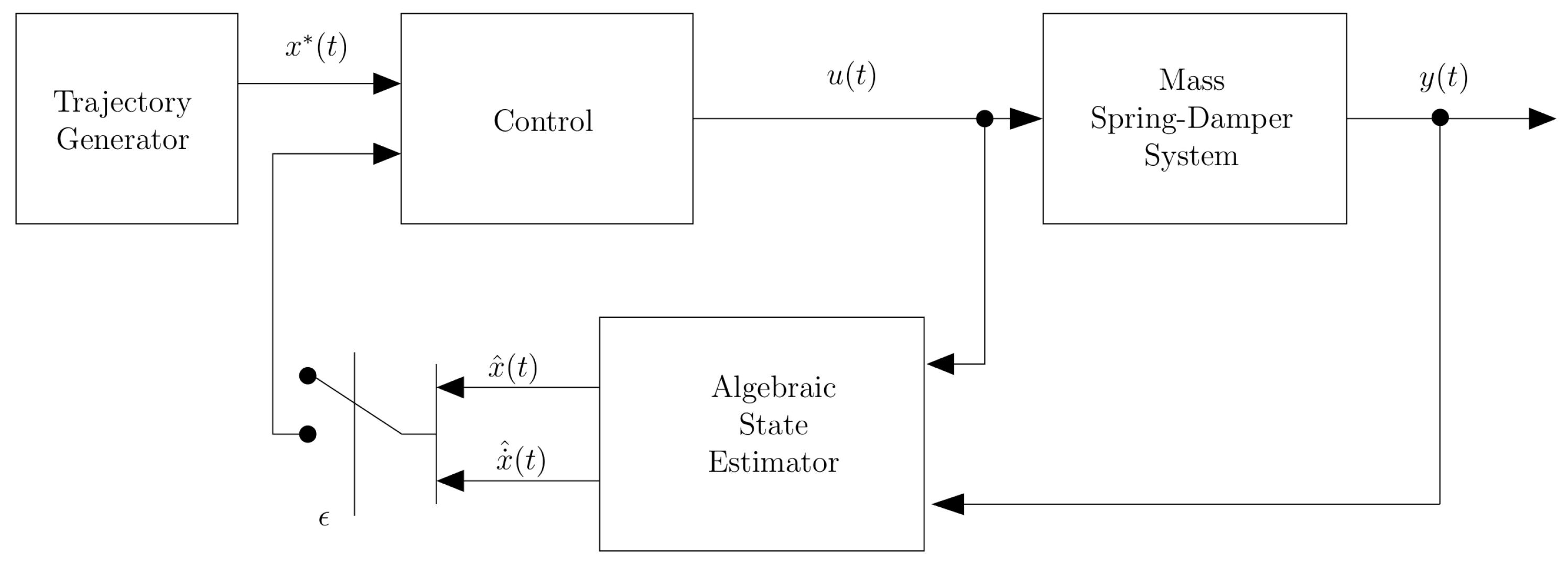
The trajectory tracking objective consists in driving the mass from an arbitrary initial position m to a final position m. In order to illustrate the accuracy of the initial condition estimation performed by the proposed algebraic estimator, the initial conditions of the system were chosen to be different from zero: m and m·s. The controlled system is depicted in Figure 1.

Figure 1.
Feedback control via output acceleration feedback and algebraic state estimation.
It is important to point out that the algebraic estimator does not require any traditional parameter tuning. In all simulations, the control gains are set as and , .
5.1. Estimation without Measurement Noise
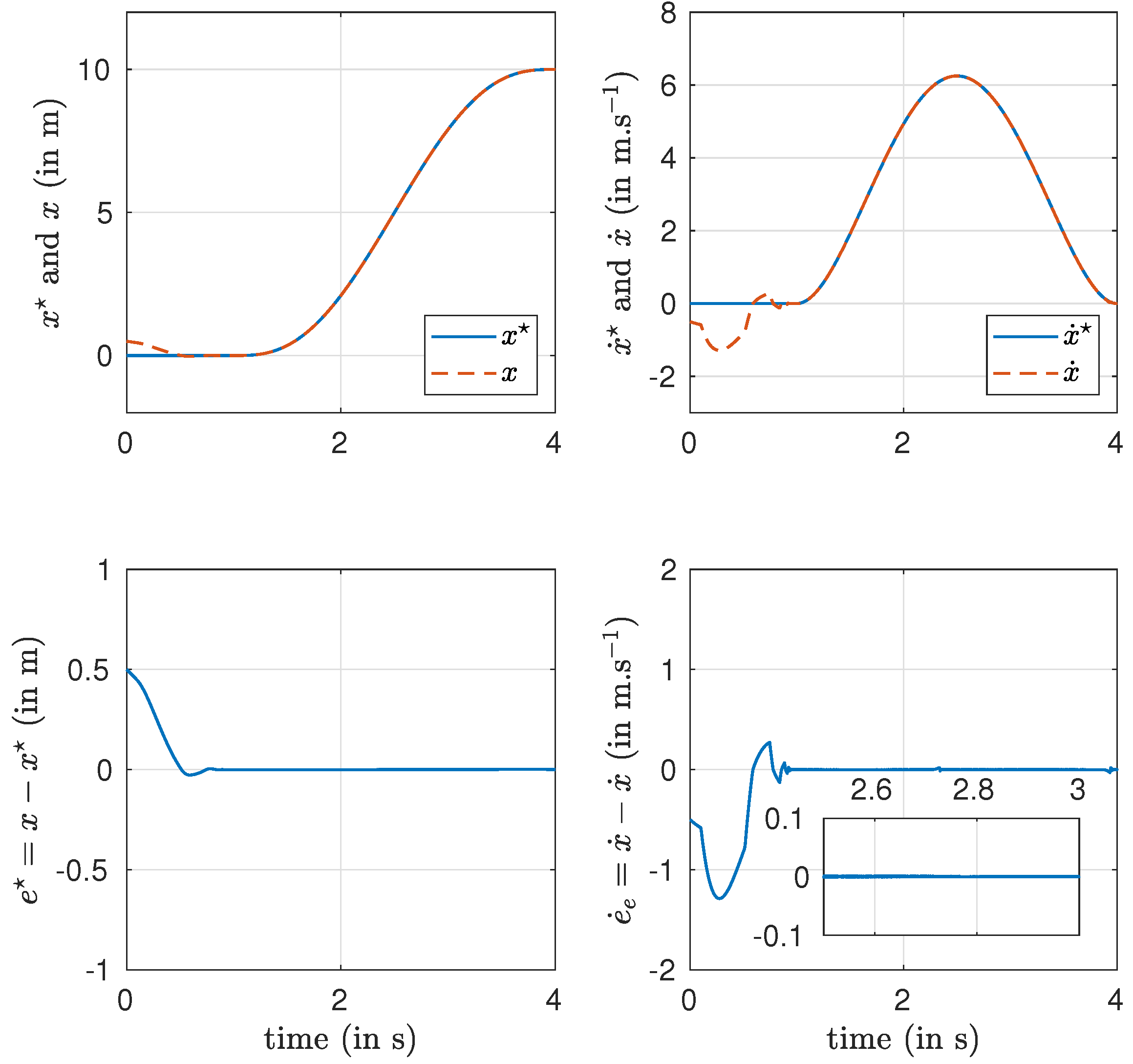
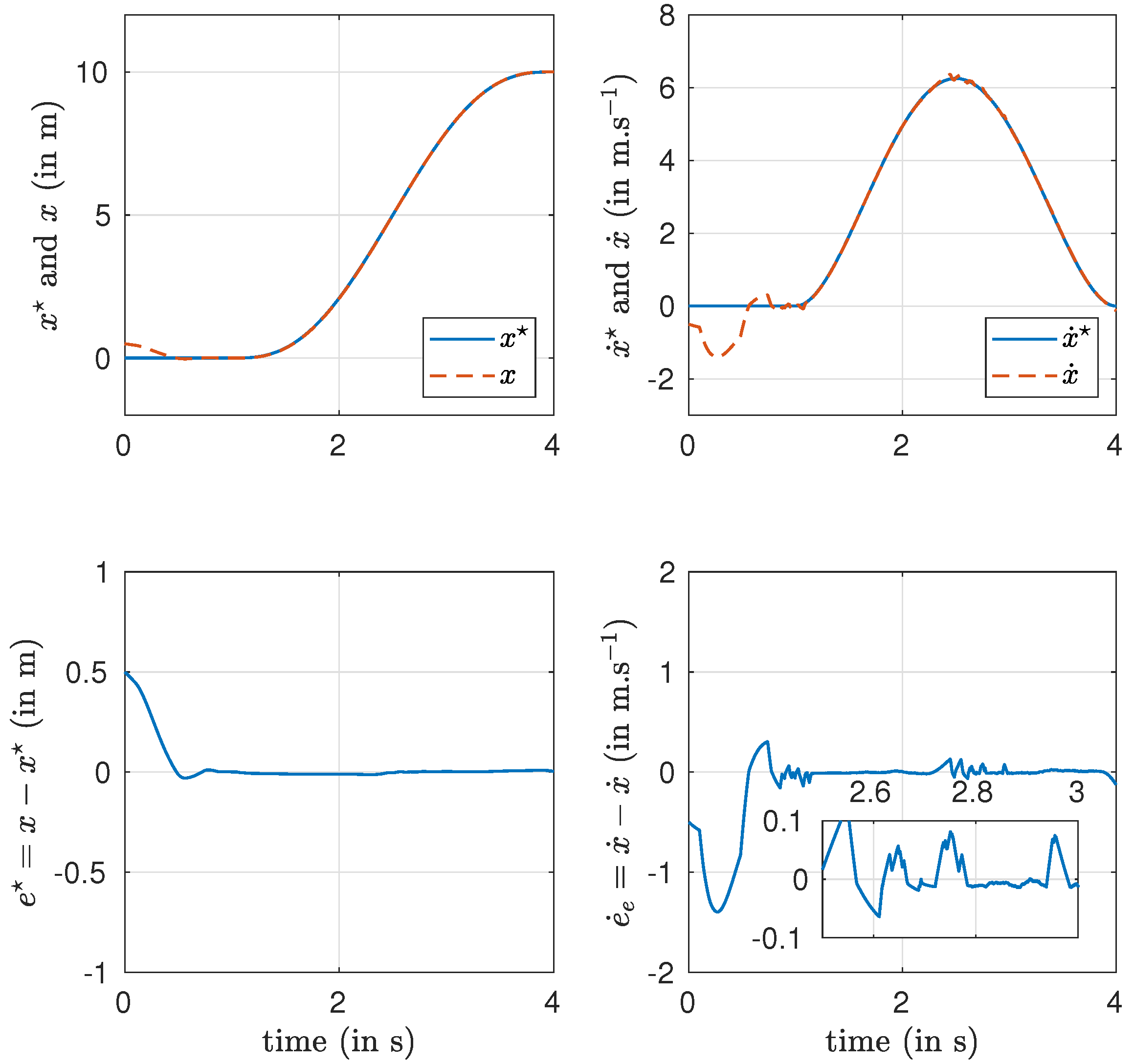
A first set of simulations is provided when the output y is not corrupted by noise. Since the estimation is not valid at , as described in Equation (12), the control is set after a small time s. In Figure 2, it can be seen that the tracking objective problem is achieved in finite time and with very good accuracy.
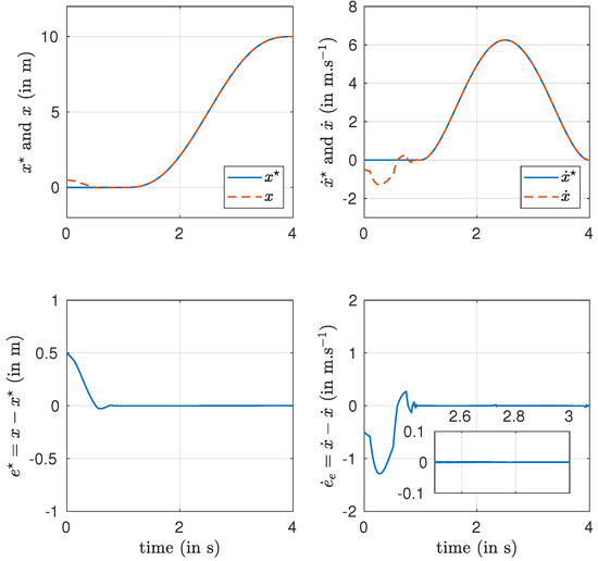
Figure 2.
Trajectory tracking and tracking errors.
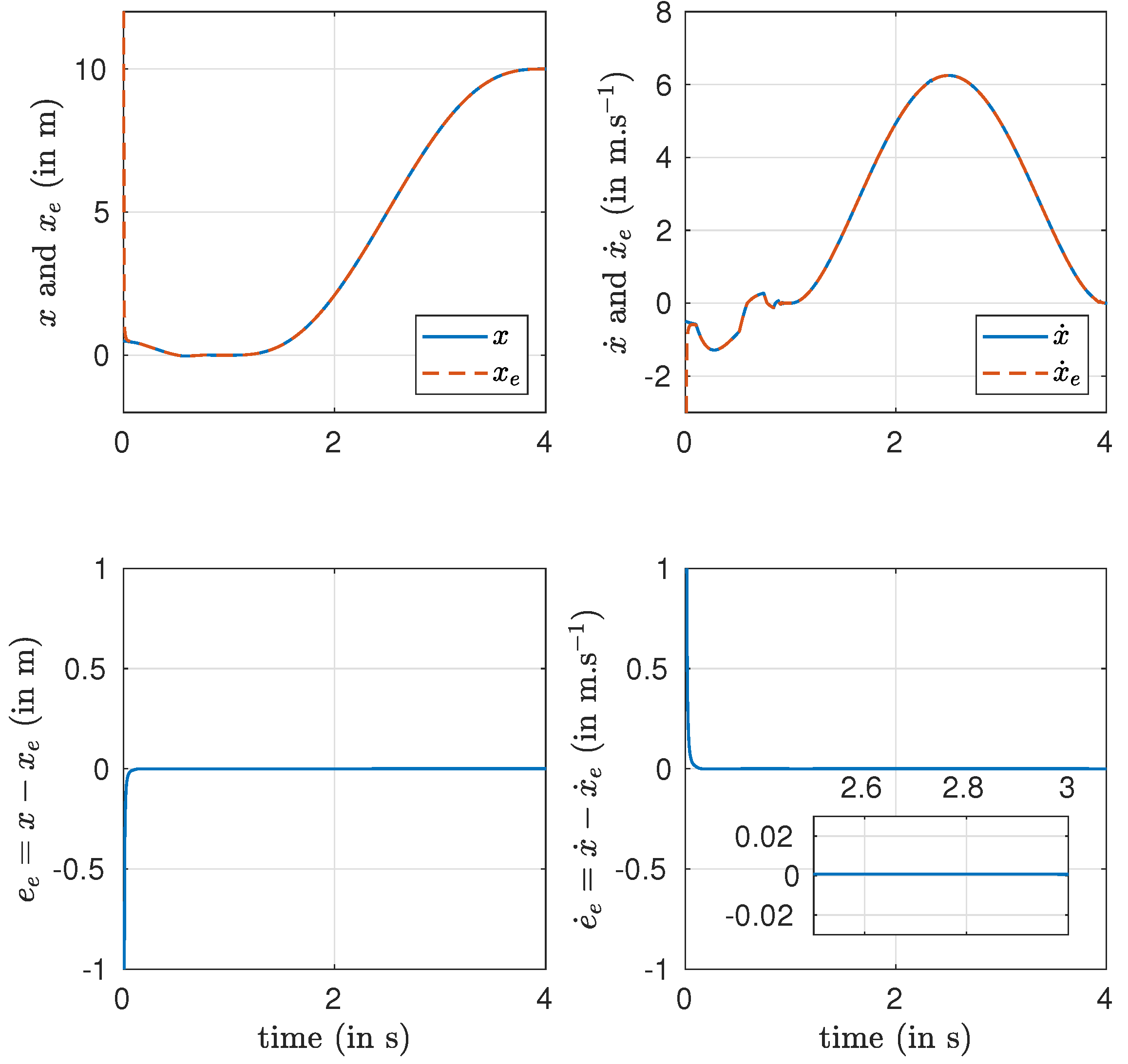
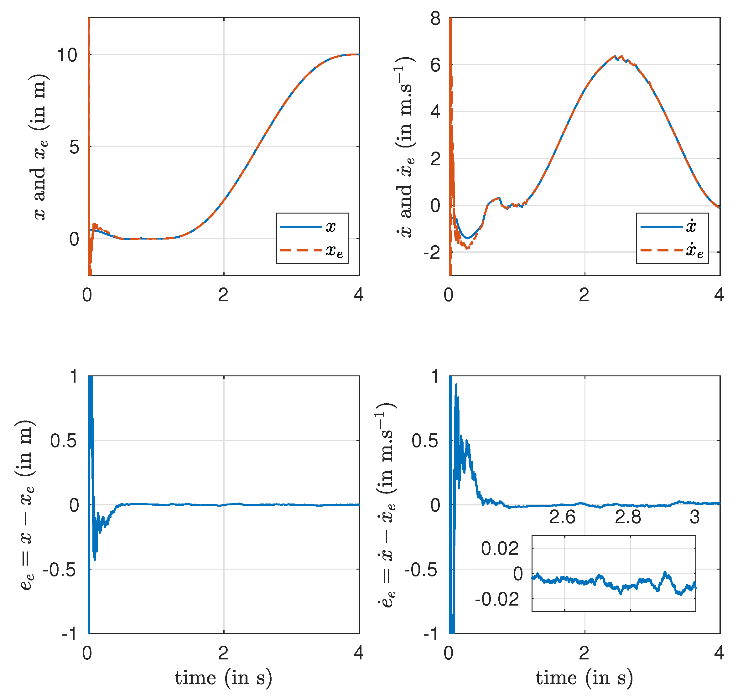
Figure 3 depicts the position and the velocity , together with their estimates and , as well as the estimation errors. In the absence of noise, one can conclude that all variables converge in finite time to their desired value thanks to the use of the algebraic estimator and the quasi-homogeneous second-order sliding mode.
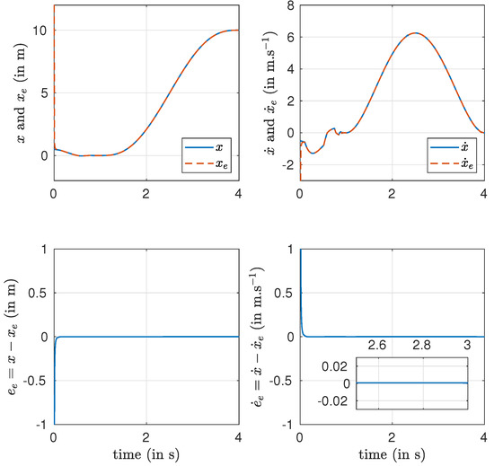
Figure 3.
Position and velocity estimation and the estimation errors.
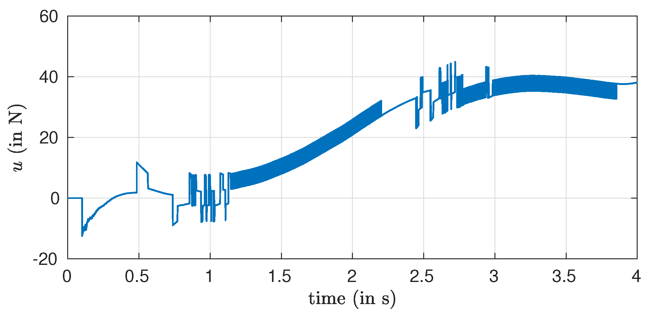
In order to highlight another feature of the integral observer, only signum functions in the sliding mode controller were used in the simulations (as it can be seen in Figure 4, whereas with other finite-time observers, continuous approximations of the controller, such as saturation or sigmoid functions, are usually implemented in order to alleviate the chattering phenomenon.
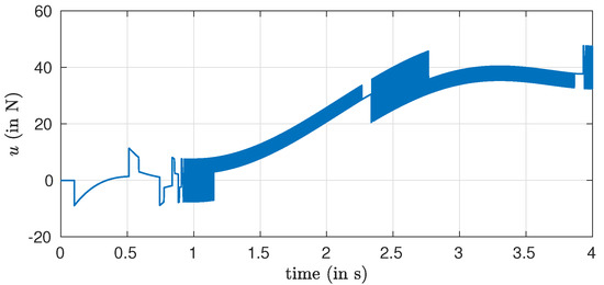
Figure 4.
Control law without noise measurement.
5.2. Estimation with Measurement Noise
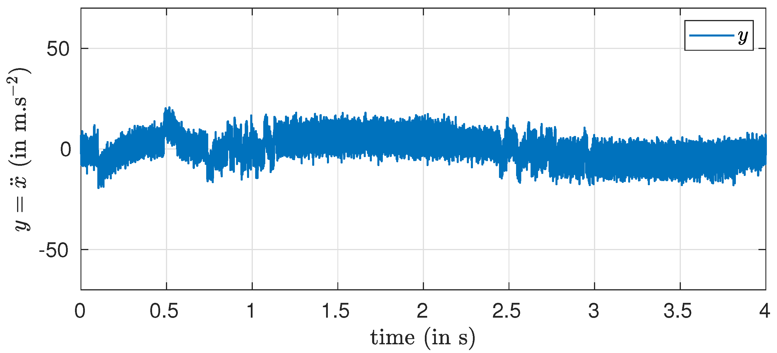
Simulations were also carried out to assess the performance of the output acceleration feedback scheme when a measurement noise process is present in the acceleration measurement. To evaluate the robustness of the proposed algorithm, a significant white noise with variance was added on the measured acceleration. The noisy measured acceleration is given in Figure 5.
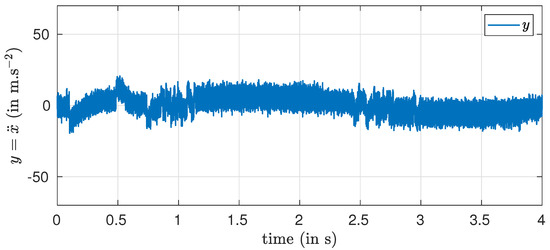
Figure 5.
Acceleration: measured output corrupted by noise.
The same simulations are performed in order to evaluate the noise influence. Figure 6 depicts the tracking behavior, in Figure 7 are given the estimate of the states and in Figure 8 is reported the control behavior.
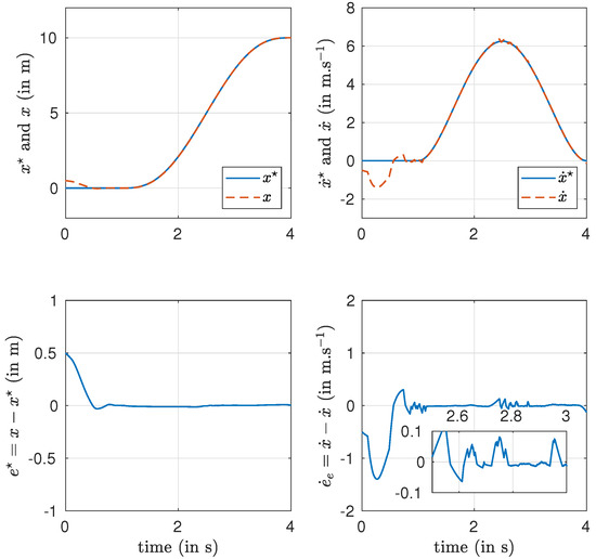
Figure 6.
Trajectory tracking and errors corrupted by noise.

Figure 7.
Position and velocity estimation and errors corrupted by noise.

Figure 8.
Control law with noise measurement.
It can be seen that despite the significant noise affecting the measurement, all controlled variables and estimates converge very fast to their desired values and with very good accuracy. The noise effect is present at the beginning of the simulations. However, as the inputs and the outputs are being integrated, these noise effects are quickly attenuated.
6. Conclusions and Future Work
In this article, we have proposed a novel approach for the finite-time feedback control of second-order systems based on the availability of the acceleration signal only. The approach uses model-based algebraic state estimation in a novel fashion. All required variables for control are obtained in finite time with only integrals of measurements multiply by powers of the time variables which overcomes the noise sensitivity problem. Only a time reset is needed to overcome the sensitivity problems which may be caused by the integration of the time variable. As a bonus, the initial conditions of the plant state and the integral of the position variable are also obtained, which could substantially ease implementation actions in the control loop. While achieving finite-time convergence, the proposed approach has definite noise processing advantages. Furthermore, with this approach the measured signals are only integrated and no parameter tuning is needed for this estimator. The closed-loop finite-time tracking was obtained using a quasi-homogeneous second-order sliding-mode observers.
The results of this article have been illustrated via numerical simulations on a second-order mass-spring-dumper system in a position reference trajectory tracking task. The simulations have shown excellent results, even in the presence of measurement noise. We have confirmed that the estimation is quite fast and occurs in a, small, finite amount of time. When measurement noise is added, the simulations have shown that the noise was also quickly attenuated by the integration structure present in the estimator. Finally, using these estimations, the designed control law exhibits an excellent performance and output tracking qualities. The tracking error is reasonably small even in the presence of measurement noises.
The proposed results might be generalized with some additional efforts. It would be interesting to apply this algorithm to a larger class of perturbed systems with possible nonlinearities. Other applications for fault sensor position and velocity detection with reconfiguration control are also under study.
Author Contributions
Conceptualization, R.D., T.F. and H.S.-R.; Data curation, R.D.; Writing—original draft, R.D., T.F. and H.S.-R.; Writing—review & editing, T.F. All authors have read and agreed to the published version of the manuscript.
Funding
This research received no external funding.
Data Availability Statement
Not applicable.
Conflicts of Interest
The authors declare no conflict of interest.
References
- Inman, D.J. Vibration with Control; Academic Press/John Wiley & Sons, Ltd.: Cambridge, MA, USA, 2006. [Google Scholar]
- Wu, Y.; Tarn, T.J.; Xi, N.; Isidori, A. On Robust Impact Control via Positive Acceleration Feedback for Robot Manipulators. In Proceedings of the IEEE International Conference on Robotics and Automation, Minneapolis, MN, USA, 22–28 April 1996; pp. 1891–1896. [Google Scholar]
- Jabbari, F.; Schmitendorf, W.; Yang, J. H∞ Control for Seismic-Excited Buildings with Acceleration Feedback. J. Eng. Mech. 1995, 9, 994–1002. [Google Scholar] [CrossRef]
- Delpoux, R.; Sira-Ramirez, H.; Floquet, T. Acceleration Feedback via an algebraic state estimation method. In Proceedings of the 52th IEEE Conference on Decision and Control, Firenze, Italy, 10–13 December 2013. [Google Scholar]
- Orlov, Y. Discontinuous Systems; Springer: Berlin/Heidelberg, Germany, 2009. [Google Scholar]
- Fliess, M.; Sira-Ramírez, H. An algebraic framework for linear identification. ESAIM Control Optim. Calc. Var. 2003, 9, 151–168. [Google Scholar] [CrossRef]
- Delpoux, R.; Floquet, T. On-line parameter estimation via algebraic method: An experimental illustration. Asian J. Control 2014, 17, 315–326. [Google Scholar] [CrossRef] [Green Version]
- Linares-Flores, J.; Sira-Ramírez, H.; Yescas-Mendoza, E.; Vásquez-Sanjuan, J.J. A comparison between the algebraic and the reduced order observer approaches for on-line load torque estimation in a unit power factor rectifier-DC motor system. Asian J. Control 2012, 14, 45–57. [Google Scholar] [CrossRef]
- Mboup, M. Parameter estimation for signals described by differential equations. Appl. Anal. Int. J. 2009, 88, 29–52. [Google Scholar] [CrossRef]
- Morales, R.; Feliu, V.; Sira-Ramírez, H. Nonlinear Control for Magnetic Levitation Systems Based on Fast Online Algebraic Identification of the Input Gain. IEEE Trans. Control Syst. Technol. 2011, 19, 757–771. [Google Scholar] [CrossRef]
- Belkoura, L.; Richard, J.P.; Fliess, M. Parameters estimation of systems with delayed and structured entries. Automatica 2009, 45, 1117–1125. [Google Scholar] [CrossRef] [Green Version]
- Belkoura, L.; Floquet, T.; Ibn Taarit, K.; Perruquetti, W.; Orlov, Y. Estimation problems for a class of impulsive systems. Int. J. Robust Nonlinear Control 2010, 21, 1066–1079. [Google Scholar] [CrossRef] [Green Version]
- Fliess, M.; Join, C.; Mboup, M. Algebraic change-point detection. Appl. Algebra Eng. Commun. Comput. 2010, 21, 131–143. [Google Scholar] [CrossRef] [Green Version]
- Mboup, M.; Join, C.; Fliess, M. Numerical differentiation with annihilators in noisy environment. Numer. Algorithm 2009, 50, 439–467. [Google Scholar] [CrossRef] [Green Version]
- Kiltz, L.; Join, C.; Mboup, M.; Rudolph, J. Fault-tolerant control based on algebraic derivative estimation applied on a magnetically supported plate. Control Eng. Pract. 2014, 26, 107–115. [Google Scholar] [CrossRef]
- Duncan, T.E.; Mandl, P.; Pasik-Duncan, B. Numerical differentiation and parameter estimation in higher-order linear stochastic systems. IEEE Trans. Autom. Control 1996, 41, 522–532. [Google Scholar] [CrossRef]
- Ibrir, S. Linear time-derivative trackers. Automatica 2004, 40, 397–405. [Google Scholar] [CrossRef]
- Bejarano, F.J.; Pisano, A.; Usai, E. Finite-Time Converging Jump Observer for Switched Linear Systems with Unknown Inputs. Nonlinear Anal. Hybrid Syst. 2011, 5, 174–188. [Google Scholar] [CrossRef]
- Ghanes, M.; Barbot, J.P.; Fridman, L.; Levant, A.; Boisliveau, R. A New Varying-Gain-Exponent-Based Differentiator/Observer: An Efficient Balance Between Linear and Sliding-Mode Algorithms. IEEE Trans. Autom. Control 2020, 65, 5407–5414. [Google Scholar] [CrossRef]
- Levant, A. Higher-order sliding modes, differentiation and output-feedback control. Int. J. Control 2003, 76, 924–941. [Google Scholar] [CrossRef]
- Levant, A.; Livne, M. Robust exact filtering differentiators. Eur. J. Control 2020, 55, 33–44. [Google Scholar] [CrossRef]
- Lopez-Ramirez, F.; Polyakov, A.; Efimov, D.; Perruquetti, W. Finite-Time and Fixed-Time Observer Design: Implicit Lyapunov Function Approach. Automatica 2018, 87, 52–60. [Google Scholar] [CrossRef] [Green Version]
- Cruz-Zavala, J.; Moreno, J.A. Levant’s arbitrary order exact differentiator: A Lyapunov approach. IEEE Trans. Autom. Control 2019, 64, 3034–3039. [Google Scholar] [CrossRef]
- Mincarelli, D.; Pisano, A.; Floquet, T.; Usai, E. Uniformly convergent sliding mode-based observation for switched linear systems. Int. J. Robust Nonlinear Control 2016, 26, 1549–1564. [Google Scholar] [CrossRef] [Green Version]
- Perruquetti, W.; Floquet, T. Homogeneous finite time observer for nonlinear systems with linearizable error dynamics. In Proceedings of the IEEE Conference on Decision and Control, New Orleans, LA, USA, 12–14 December 2007. [Google Scholar] [CrossRef] [Green Version]
- Wang, Y.; Zheng, G.; Efimov, D.; Perruquetti, W. Differentiator application in altitude control for an indoor blimp robot. Int. J. Control 2018, 91, 2121–2130. [Google Scholar] [CrossRef] [Green Version]
- Diop, S.; Fliess, M. Nonlinear observability, identifiability and persistent trajectories. In Proceedings of the 36th IEEE Conference on Decision and Control, Brighton, UK, 11–13 December 1991; pp. 714–719. [Google Scholar]
- Riachy, S.; Orlov, Y.; Floquet, T.; Santiesteban, R.; Richard, J.P. Second order sliding mode control of underactuated Mechanical systems I: Local stabilization with application to an inverted pendulum. Int. J. Robust Nonlinear Control 2008, 18, 529–543. [Google Scholar] [CrossRef] [Green Version]

Publisher’s Note: MDPI stays neutral with regard to jurisdictional claims in published maps and institutional affiliations. |
© 2021 by the authors. Licensee MDPI, Basel, Switzerland. This article is an open access article distributed under the terms and conditions of the Creative Commons Attribution (CC BY) license (https://creativecommons.org/licenses/by/4.0/).