Unsupervised Deep Learning-Based Network Traffic Anomaly Detection for DDoS Mitigation in Smart Microgrid Communication Infrastructure

Abstract

Smart microgrids depend on continuous communication between controllers, sensors, and actuators over industrial protocols like Modbus TCP, message queuing telemetry transport (MQTT), and distributed network protocol 3 (DNP3), which were designed without built-in security mechanisms. The gateway that aggregates this traffic represents a single point of failure and is vulnerable to distributed denial-of-service (DDoS) attacks. Most existing detection methods require labeled attack data for training, a condition rarely met in operational technology (OT) environments. This paper presents an unsupervised convolutional neural network–long short-term memory (CNN-LSTM) model trained exclusively on normal microgrid gateway traffic to predict the next traffic window; anomalies are flagged when the prediction error exceeds a threshold derived from the training distribution. A dual-branch architecture processes metric time-series through LSTM layers and flow aggregate features through CNN layers, fusing both representations for prediction. The model is evaluated against three protocol-specific DDoS attack scenarios—Modbus supervisory control and data acquisition (SCADA) flooding, MQTT publish storm, and DNP3 response flooding—none of which are seen during training. Compared against an isolation forest baseline and an autoencoder baseline under identical unsupervised conditions, the CNN-LSTM achieves higher precision and recall on all attack types. The framework is deployed within a web-based monitoring platform that supports real-time detection and anomaly logging.

1. Introduction

Microgrids are localized energy systems that integrate distributed energy resources—solar inverters, battery storage, wind turbines—with loads and controllers into a coordinated network. These systems rely on continuous data exchange between field devices and a central controller through a shared communication infrastructure. The protocols carrying this data are Modbus TCP, message queuing telemetry transport (MQTT), and distributed network protocol 3 (DNP3), designed for reliability in isolated industrial networks, not for security in internet protocol (IP)-connected environments. Modbus TCP transmits register values in plaintext over port 502. MQTT brokers in many deployments accept connections with minimal credential verification. DNP3 outstations, in turn, respond to any master that sends a correctly formatted request. The microgrid gateway, which aggregates all device communication onto a single network interface, becomes a natural target for distributed denial-of-service (DDoS) attacks. A sustained flood directed at the gateway saturates the communication channel, silences sensor telemetry, and disrupts real-time control, which potentially causes cascading failures across connected loads [1,2,3,4].

A growing body of research addresses intrusion detection for smart grids and supervisory control and data acquisition (SCADA) networks, but the dominant approaches rely most of the time on supervised learning with labeled attack data. Classifiers trained on datasets such as CIC-IDS2017, NSL-KDD, or UNSW-NB15 achieve high accuracy on those benchmarks, yet these datasets contain enterprise IT traffic with no representation of operational technology (OT) protocols like Modbus TCP or DNP3. The traffic patterns in a microgrid—periodic polling, deterministic timing, and protocol-specific function codes—differ fundamentally from web browsing or email flows. Supervised methods also assume that representative attack samples exist for every threat, and specifically in operational microgrids, novel attack variants targeting OT protocol quirks may appear without any prior signature. Most existing work focuses on a broad SCADA or wide-area monitoring system (WAMS) scope rather than the microgrid gateway communication layer specifically. This leaves a gap: no detection framework that operates without labeled attack data targets the microgrid gateway and processes OT protocol traffic at the network level [5,6,7,8,9,10].

In our prior work [1], we developed an autoencoder-based anomaly detection system for monitoring microgrid sensor data, including current, voltage, and communication traffic, achieving 98% recall and 96.08% precision. While effective for device-level anomaly detection, that approach treated communication traffic as a single aggregated metric without protocol-level differentiation or flow-level analysis. A Modbus TCP polling anomaly and an MQTT subscription flood would produce similar aggregate traffic spikes, indistinguishable to the autoencoder. The present work extends our research by performing deep, protocol-aware network traffic analysis in the microgrid gateway layer.

This paper proposes an unsupervised convolutional neural network–long short-term memory (CNN-LSTM) framework trained exclusively on normal OT traffic captured at the microgrid gateway. The model learns to predict the next traffic window from sequences of normal Modbus TCP, MQTT, and DNP3 traffic; anomalies are flagged when the prediction error exceeds a learned threshold. Three protocol-specific DDoS attack scenarios are evaluated at test time only, and the model never sees attack traffic during training. An isolation forest baseline and an autoencoder baseline are trained under identical unsupervised conditions, receiving the same input features, to provide fair comparisons against both traditional unsupervised machine learning and an additional unsupervised deep learning approach. A complete detection pipeline is deployed within a web-based monitoring platform that receives traffic in real time, performs feature extraction, runs inference, and logs detected anomalies.

The main contributions of this work are as follows:

• An unsupervised detection approach requiring no labeled attack data, trained exclusively and specifically on normal microgrid gateway traffic;
• An explicit focus on the microgrid gateway communication layer, where Modbus TCP, MQTT, and DNP3 traffic converges;
• A synthetic OT-protocol-aware dataset with traffic parameters grounded in published protocol specifications;
• A comparative evaluation between the proposed deep learning model (CNN-LSTM) and unsupervised baselines (autoencoder and isolation forest) under identical conditions;
• Full system-level integration with a real-time monitoring platform supporting live anomaly detection and logging.

This is how this study is structured. Section 2 presents the materials and methods, including related work (Section 2.1), the system architecture and data generation (Section 2.2), the detection methodology (Section 2.3), and the experimental setup (Section 2.4). Section 3 reports and discusses the results, and Section 4 concludes this paper with future directions.

2. Materials and Methods

2.1. Related Work

2.1.1. DDoS Detection in Smart Grid and Microgrid Environments

Diaba and Elmusrati [2] proposed a CNN-gated recurrent unit (GRU) hybrid for smart grid DDoS detection, training on a custom dataset that combines normal smart grid traffic with labeled attack traces. Their model achieved 97% detection accuracy, but it depends entirely on supervised training, which means the classifier can only recognize attack patterns present in the training set. When a DDoS variant not represented in the training distribution targets a microgrid, this approach fails silently.

Naqvi et al. [3] addressed a related problem using reconstructive machine learning models, including autoencoders and variational autoencoders, for DDoS detection in smart grid networks. Their reconstruction-based approach is conceptually closer to unsupervised detection since the model learns to reconstruct normal traffic and flags deviations. However, their evaluation was limited to generic TCP/IP traffic, without any OT protocol specific to their feature set, like Modbus TCP function codes, MQTT message types, and DNP3 data objects.

AlHaddad et al. [4] proposed a CNN+GRU model that included a monitoring dashboard for smart grid intrusion detection, published in MDPI’s Sensors. The ensemble architecture improved detection stability across attack types, but all ensemble components still require labeled training data. Hosseini Rostami et al. [5] took a different angle, applying a transformer+LSTM approach with a Kalman filter estimator to enhance the resilience of distributed DC microgrids against cyber-attacks. Their work operates in the physical layer (state estimation) rather than the network traffic layer, which is complementary to our approach but does not address DDoS traffic flooding at the communication gateway.

None of these works target the microgrid gateway communication layer specifically, using unsupervised detection with OT protocol-aware traffic modeling.

2.1.2. Deep Learning for Network Anomaly Detection

CNN-LSTM hybrid architectures have shown strong results across network anomaly detection benchmarks. Halbouni et al. [6] proposed a CNN-LSTM hybrid for network intrusion detection, evaluating on the CICIDS2017 dataset and achieving 97.26% accuracy. Their architecture applies 1D convolution followed by LSTM layers, a pattern we adapt in our dual-branch design, though we separate the CNN and LSTM branches to process different feature types rather than chaining them sequentially.

Altunay and Albayrak [7] developed a CNN+LSTM system for industrial IoT intrusion detection, demonstrating that the hybrid outperforms standalone architectures on heterogeneous IoT traffic. Abdallah et al. [8] applied CNN-LSTM to anomaly detection in software-defined networks (SDNs). Sinha et al. [9] reported a high-performance LSTM-CNN architecture for IoT environments, and Alashjaee [10] added an attention mechanism to the CNN-LSTM pipeline, achieving sub-35 ms real-time inference latency. These works collectively validate CNN-LSTM as a viable architecture for network anomaly detection. But all five require labeled attack data for supervised training, which limits their applicability to operational OT environments where such data do not exist.

2.1.3. Unsupervised Anomaly Detection for Industrial Control Systems

Unsupervised approaches to industrial control system (ICS) anomaly detection have gained attention as researchers have recognized that labeled attack data are scarce in operational environments. Choi and Kim [11] presented an unsupervised autoencoder approach for ICS anomaly detection without label data (MDPI, Applied Systems Innovation, 2024), demonstrating that a composite autoencoder model can effectively identify anomalous patterns in both value and time dimensions using the HAI dataset, but the approach has not yet been validated against deep learning alternatives on complex traffic patterns. Altaha and Hong [12] developed unsupervised anomaly detection for DNP3 SCADA systems using function code frequency analysis (MDPI, Electronics, 2022), demonstrating that protocol-specific features improve detection over generic network statistics. Zare et al. [13] presented a real-time LSTM sequence-to-sequence autoencoder for Modbus/TCP SCADA anomaly detection evaluated on the SWaT dataset (IJCIP, 2024), prioritizing low inference latency. Ha et al. [14] applied an explainable LSTM–autoencoder one-class support vector machine (OCSVM) model for anomaly detection in industrial control systems (IFAC, 2022), adding interpretability through gradient Shapley additive explanations (SHAP)-based visualization to address the black-box limitation of deep learning approaches. The entropy-based analysis of Modbus over TCP traffic in [15] (MDPI, Journal of Cybersecurity and Privacy, 2023) showed that protocol-aware feature engineering, particularly function code distributions and timing characteristics, improves anomaly discrimination. In our prior work [1], we applied an autoencoder to device-level microgrid monitoring, treating communication traffic as a single aggregated feature.

No existing work combines unsupervised deep learning with OT protocol-aware dual-layer traffic modeling (time-series metrics and per-device flow records) for microgrid communication security. This gap motivates the present work: an unsupervised CNN-LSTM trained on normal multi-protocol OT traffic (Modbus TCP, MQTT, and DNP3) for DDoS detection, deployed within an operational monitoring platform.

To summarize, existing works fall into one or more of four categories that limit their applicability to microgrid gateway security: they require supervised training with labeled attack data, they evaluate on generic IT datasets without an OT protocol context, they target a broad SCADA or WAMS scope rather than the microgrid gateway specifically, or they provide model-only results without platform integration for operational deployment. This paper addresses all four gaps simultaneously.

2.2. System Architecture and Data Generation

2.2.1. Platform Architecture

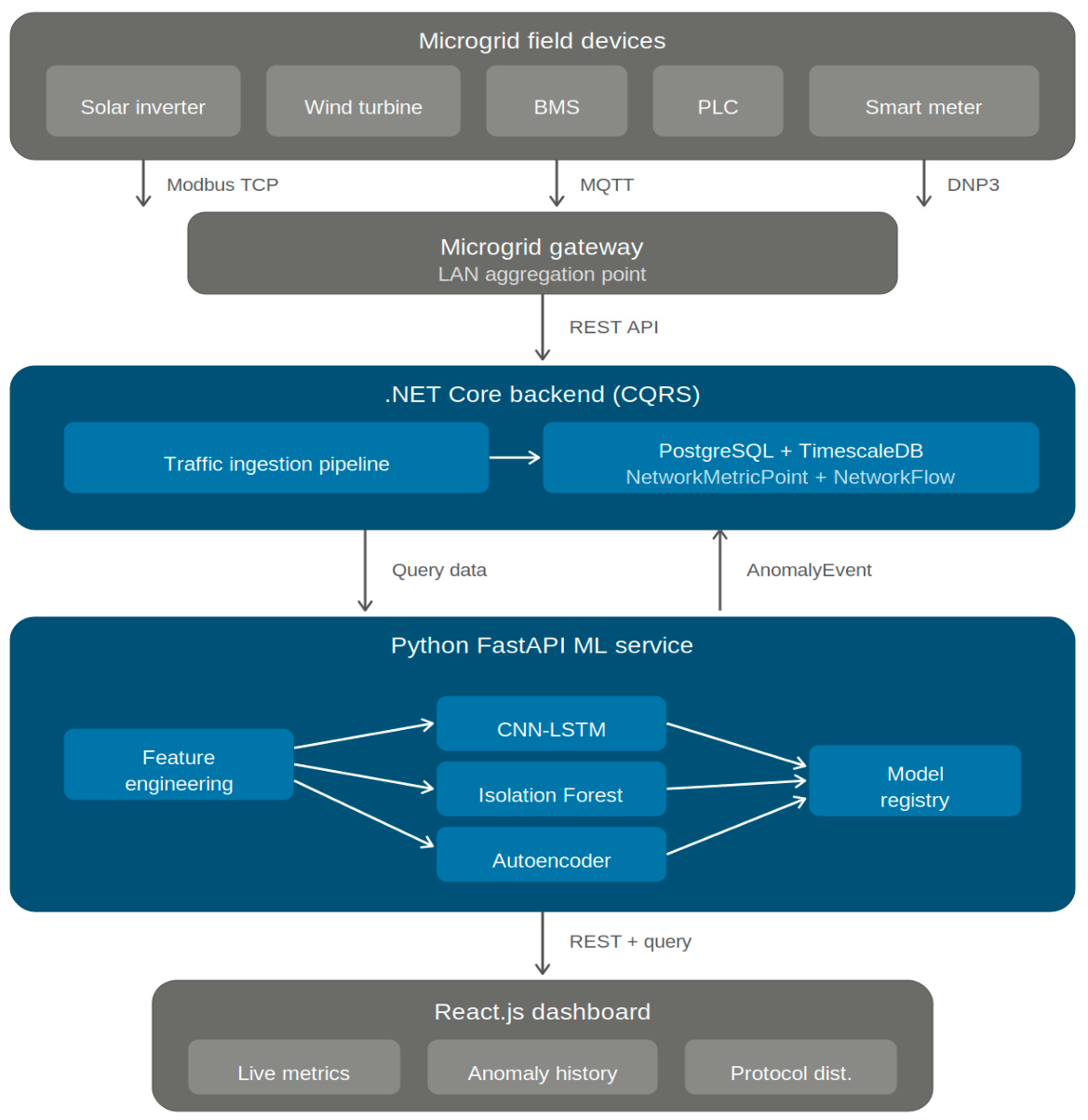
The detection framework operates within a 3-tier monitoring platform, displayed in Figure 1. The backend is built on a .NET Core (Microsoft Corporation, Redmond, WA, USA) using the Command Query Responsibility Segregation (CQRS) pattern with PostgreSQL (PostgreSQL Global Development Group, open-source software) and the TimescaleDB (Timescale, Inc., New York, NY, USA) extension providing time-series-optimized storage. Two hypertables store the incoming data: NetworkMetricPoint for aggregated gateway metrics and NetworkFlow for per-device flow records, both ingested in real time through the representational state transfer (REST) application programming interface (API). The machine learning (ML) tier is a Python FastAPI (open-source software, FastAPI project) service that hosts a model registry and a feature engineering pipeline, and inference endpoints for the CNN-LSTM, the autoencoder, and the isolation forest models. The frontend is a React.js (Meta Platforms, Inc., Menlo Park, CA, USA) dashboard displaying live metrics, anomaly history and protocol distributions.

The platform supports dual-domain detection. As shown in Figure 1, microgrid field devices like solar inverters, wind turbines, battery management systems (BMSs), PLCs, and smart meters communicate through the gateway via Modbus TCP, MQTT, and DNP3. In our prior work [1], we developed an autoencoder for device-level electrical anomaly detection, monitoring current, voltage, and aggregated communication statistics per device. That model and the CNN-LSTM presented in this paper operate concurrently: the autoencoder detects device-level anomalies, while the CNN-LSTM detects gateway-level network traffic anomalies. Detected anomalies are stored as AnomalyEvent records in PostgreSQL. The model registry allows independent versioning and activation of each model per gateway, so operators can deploy, update, or disable detection models without affecting the rest of the platform.

2.2.2. Microgrid Communication Model

The gateway interface captures two complementary layers of data. Layer 1 consists of time-series network metrics, which are latency, throughput, packet loss, jitter, and bandwidth utilization, sampled at 2 s intervals and stored as NetworkMetricPoint records. These metrics characterize the aggregate health of the communication channel. Layer 2 consists of per-device network flow records stored as NetworkFlow entries, capturing source and destination IPs, the OT protocol used, bytes and packets transferred in each direction, and flow duration. Both layers share the same gateway identifier and timestamp, allowing correlation between aggregate channel conditions and individual device behavior.

Table 1. Time-series network metrics specifications (stored as NetworkMetricPoint).

Feature	Description	Unit	Sampling Rate
Latency	Round-trip communication delay	ms	2 s
Throughput	Data transfer rate at gateway interface	Mbps	2 s
Packet Loss	Proportion of packets dropped	%	2 s
Jitter	Inter-arrival time variation	ms	2 s
Bandwidth Utilization	Proportion of available bandwidth in use	%	2 s

specifies the five metric features and their sampling characteristics, and

Table 2. Per-device network flow record specification (stored as NetworkFlow).

Field	Description	Type	Example
SrcIp	Source IP address	String	192.168.1.10
DstIp	Destination IP address	String	203.0.113.50
Protocol	OT protocol identifier	String	Modbus/MQTT/DNP3
BytesIn	Bytes received	Integer	-
BytesOut	Bytes sent	Integer	-
PacketsIn	Packets received	Integer	-
PacketsOut	Packets sent	Integer	-
TsStart	Flow start timestamp	Datetime	-
TsEnd	Flow end timestamp	Datetime	-
FlowDuration	TsEnd—TsStart	Seconds	-

details the per-device flow record fields. This dual-layer representation is central to our detection approach: the LSTM branch models temporal patterns in the metric time-series, while the CNN branch extracts spatial patterns from the flow aggregate features.

2.2.3. Synthetic Traffic Generation

The microgrid gateway simulator generates the OT network traffic used in this research. Each simulated device uses exactly one OT protocol, Modbus TCP, MQTT or DNP3 fixed at the configuration time, which reflects how real microgrid hardware operates. A solar inverter communicating via Modbus TCP does not switch to MQTT middle operation. Under normal conditions, each device generates one flow per 2 s tick. The protocol distribution in the dataset is, therefore, determined by the per-device assignment rather than by fixed ratios.

Traffic patterns are grounded in the respective protocol specification. Sensor telemetry values follow realistic profiles, solar generation follows a bell curve driven by irradiance data from the Open-Meteo (Open-Meteo, Bürs, Austria) API, the battery state of charge varies with generation and load, and building load follows weekday occupancy patterns. Network metrics are correlated with traffic volume, like throughput scales with flow byte counts, latency increases under load, and jitter reflects packet timing variance.

Table 3. Protocol-specific normal traffic parameters.

Parameter	Modbus TCP	MQTT	DNP3
Polling interval	1–5 s	Event-driven	2–10 s
Typical packet size	60–260 bytes	50–1500 bytes	10–292 bytes
Function codes/message types	FC 03, 04 (read)	PUBLISH and SUBSCRIBE	Integrity poll; event class
Specification reference	[16]	[17]	[18]

lists the protocol-specific parameters.

The simulator parameters, which include polling rates, packet sizes, flow distributions, and protocol-specific timing, are grounded in publicly documented OT protocol specifications: the Modbus TCP/IP specification [16], the MQTT v5.0 standard [17], and the IEEE 1815 DNP3 standard [18]. Representative microgrid communication profiles from the literature informed the parameter ranges. All simulation assumptions and parameters are documented in this section to enable reproducibility.

2.2.4. Attack Scenario Generation

Three protocol-specific DDoS attack scenarios are injected during tested time evaluation only. Attack traffic is never included in the training set; the models learn exclusively from normal data. Each attack scenario targets a specific OT protocol and modifies traffic characteristics that are measurable at the gateway interface. The attacking state is managed by a singleton service that controls per gateway injection timing and intensity. During attack periods, attack traffic is mixed with ongoing normal traffic to simulate realistic conditions where legitimate communication continues alongside the attack.

Table 4. Attack scenario specifications and traffic signatures.

Attack Scenario	Protocol	Traffic Signature	Metric Impact
Modbus SCADA Flooding	Modbus TCP	Few sources, large flows, bandwidth saturation, and disrupted polling regularity	BandwidthUtil 90–100%; high PacketLoss + Latency
MQTT Publish Storm	MQTT	Many sources, small flows, packet explosion, and quality of service (QoS) shift	Moderate BandwidthUtil; high PacketCount
DNP3 Response Flooding	DNP3	Multi-source burst, small packets, high jitter, and timing deviation	Very high jitter; sharp latency spike

specifies each scenario, and

Table 5. Quantitative attack traffic parameters per scenario, sourced from the gateway simulator implementation (SimulatorBackgroundService).

Scenario	Packet Rate (pkt/s)	Burst Duration (s)	Source IPs	Attack-to-Normal Ratio	Parameter Rationale
Modbus SCADA flooding	800–1200	30–60	3–5	≈6:1	Volumetric Modbus/TCP flood pattern characterized by Bhatia et al., with rate scaled to a 1 Mbps gateway link [19]
MQTT publish storm	250–400	20–45	8–15	≈4:1	Multi-source MQTT broker overload pattern (CONNECT- and PUBLISH-flood family); detection setting motivated by the DoS/DDoS-MQTT-IoT dataset of Alatram et al. [20]
DNP3 response flooding	150–300	15–30	2–4	≈3:1	Unsolicited-response flooding pattern modeled after the event-buffer flooding attack of Jin et al., exploiting the unsolicited-response mechanism defined in IEEE 1815-2012 [21]

specifies quantitative attack traffic parameters per scenario.

2.3. Detection Methodology

The assumption already underlying this work is that, in real-world microgrid deployments, operators have abundant normal operating data but little to no labeled attack data. An energy management system that has been running for months accumulates tens of thousands of normal traffic windows; labeled examples of Modbus SCADA floods or DNP3 response flooding are, in practice, unavailable. The detection framework is, therefore, designed around an unsupervised paradigm: all five evaluated models (CNN-LSTM, LSTM-only, CNN-only, autoencoder, and isolation forest) are trained exclusively on normal traffic data. During operation, any incoming traffic that deviates from learned normal patterns beyond a threshold is flagged as anomalous. This design choice ensures direct applicability to production microgrid environments without requiring attack-specific training data.

During the training phase, the CNN-LSTM learns to predict the next traffic window from sequences of normal Modbus, MQTT, and DNP3 traffic. The autoencoder learns to compress and reconstruct normal traffic windows through a bottleneck representation. The isolation forest learns the density and structure of the normal traffic feature space. No attack data, no labels, and no attack signatures are used during training. During the detection phase, protocol-specific DDoS flooding attacks are simulated at test time only, representing previously unseen anomalies. The CNN-LSTM flags anomalies when the prediction error exceeds a threshold derived from the normal training distribution. The autoencoder flags anomalies when the per-window reconstruction error exceeds a threshold derived from the training reconstruction error distribution. The isolation forest flags anomalies when data points fall in low-density regions of the learned normal feature space. None of the models has seen any attack patterns during training, and detection is based purely on deviation from normal.

2.3.1. Feature Engineering

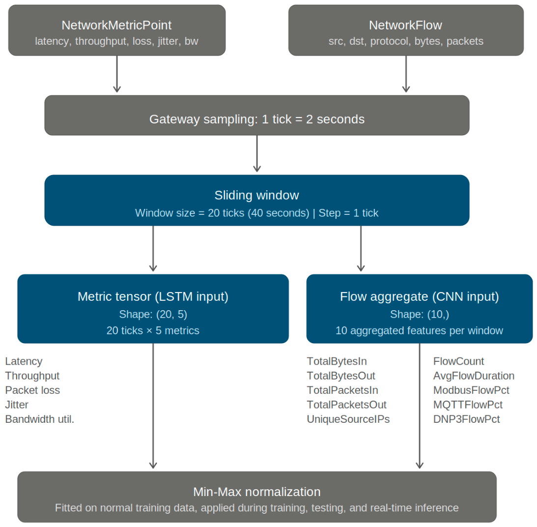
Raw data from both layers are transformed into fixed-size input windows using a sliding window approach, as shown in Figure 2. The gateway samples at 1 tick = 2 s. The window size is 20 ticks (40 s at the 2 s sampling interval), and the window step is 1 tick, creating overlapping windows that capture gradual traffic changes. We selected 20 ticks because it provides enough temporal context for the LSTM to observe multiple polling cycles across all three protocols, where there are at least 8 Modbus polls at 5 s intervals, several MQTT events, and 4–20 DNP3 responses, while keeping the computational cost manageable.

Each window produces two inputs for the model. The metric tensor has shape (20, 5), containing 20 timesteps of 5 metric features: latency, throughput, packet loss, jitter, and bandwidth utilization. The flow aggregate vector has shape (10,), computed by aggregating all flow records within the window: TotalBytesIn, TotalBytesOut, Total-PacketsIn, TotalPacketsOut, UniqueSourceIPs, FlowCount, AvgFlowDuration, Mod-busFlowPct, MQTTFlowPct, and DNP3FlowPct. The last three features capture the protocol distribution within each window. A Modbus-heavy window has a different flow profile than an MQTT-heavy one, and a DDoS attack targeting one protocol shifts this distribution. All features are normalized to [0, 1] using Min–Max scaling fitted on the normal training data.

2.3.2. CNN-LSTM Architecture (Proposed Model)

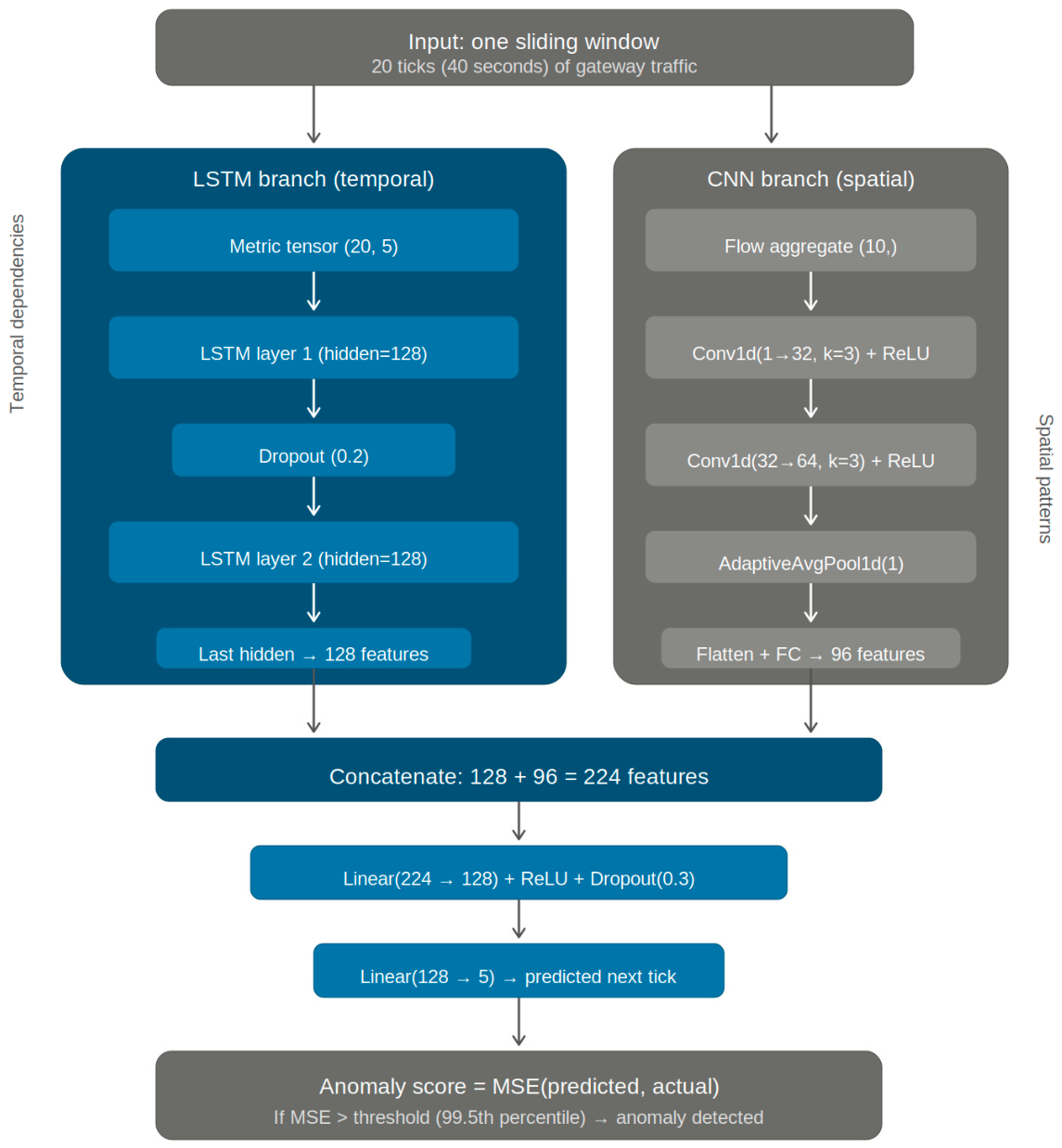
The proposed model uses a dual-branch architecture that processes the two input types through separate branches before fusing them for prediction, as illustrated in Figure 3. The LSTM branch (left side of Figure 3) processes the metric tensor, capturing temporal dependencies across the 20-timestep window. The CNN branch (right side of Figure 3) processes the flow aggregate vector, extracting spatial patterns across the 10 flow features. The two branches are fused through concatenation followed by dense layers. The model operates in a prediction-based anomaly detection mode, in which it predicts the next tick’s 5 metric values, and the anomaly score is computed as mean squared error (MSE) (predicted, actual). If the MSE exceeds the threshold (99.5th percentile of the training distribution), the window is flagged as anomalous.

The CNN branch receives the flow aggregate vector of shape (10,), reshaped to (1, 10) for 1D convolution. Two convolutional layers are applied: Conv1d (in_channels=1, out_channels=32, kernel_size=3) followed by rectified linear unit (ReLU) activation, then Conv1d (in_channels=32, out_channels=64 kernel_size=3) followed by a ReLU. An AdaptiveAvgPool1d(1) layer reduces the spatial dimension to a single value per channel, followed by flattening to a 64-dimensional vector and a fully connected layer Linear (64, 96) that produces a 96-dimensional feature vector. This branch learns which combinations of flow features co-occur under normal conditions, for instance, the relationship between ModbusFlow packets, TotalBytesIn, and UniqueSource IPs during routine polling.

The LSTM branch receives the metric tensor of shape (20, 5). A 2-layer LSTM with a hidden size of 128, dropout of 0.2, and batch_first=True processes the 20-step sequence. The last hidden state is extracted, producing a 128-dimensional feature vector. The LSTM captures how the 5 metric features evolve over a 40 s window. Normal traffic produces predictable latency and throughput trajectories, while DDoS attacks disrupt these patterns over consecutive timesteps. The LSTM cell operations follow the standard formulation [22].

The fusion layer concatenates the CNN output (96 features) and the LSTM output (128 features) into a 224-dimensional vector. This vector passes through Linear (224, 128) with ReLU activation and Dropout (0.3), and then Linear (128, 5) to produce the predicted next-tick metric values. The training objective is to minimize the mean squared error between predicted and actual next-tick metrics across all windows in the normal training set.

2.3.3. Anomaly Threshold Determination

After training, the CNN-LSTM is run on the normal training set to generate predictions for every training sample. The MSE between predicted and actual next-tick metrics is computed for each window:

$$\mathit{M}\mathit{S}\mathit{E}={\displaystyle \frac{1}{\mathit{n}}}\sum _{\mathit{i}}{\left({\mathit{x}}_{\mathit{i}}-{\widehat{\mathit{x}}}_{\mathit{i}}\right)}^2$$

(1)

where $\mathit{n}$ = 5 is the number of predicted metrics, ${\mathit{x}}_{\mathit{i}}$ is the actual value of the $\mathit{i}$ metric, and ${\widehat{\mathit{x}}}_{\mathit{i}}$ is the corresponding predicted value. The anomaly threshold is set at the 99.5th percentile of this training MSE distribution:

$$\mathsf{\theta }={\mathit{P}}_{99.5}\left({\mathit{M}\mathit{S}\mathit{E}}_{\mathit{t}\mathit{r}\mathit{a}\mathit{i}\mathit{n}}\right)$$

(2)

where $\mathsf{\theta }$ is the anomaly threshold, and ${\mathit{M}\mathit{S}\mathit{E}}_{\mathbf{t}\mathbf{r}\mathbf{a}\mathbf{i}\mathbf{n}}$ gives the set of prediction errors computed on the normal training data. At inference time, any window whose prediction error exceeds $\mathsf{\theta }$ is flagged as anomalous. We chose a percentile-based threshold rather than fixed multiple standard deviations because the MSE distribution is right-skewed; normal traffic occasionally produces larger prediction errors during communication gaps or retransmission bursts. The 90th, 95th, 97th, and 99th percentiles are also evaluated in the ablation study (Section 3.4).

2.3.4. Isolation Forest Baseline

Isolation forest [23] serves as the unsupervised traditional ML baseline. The algorithm detects anomalies by recursively partitioning the feature space with random splits, where data points that require fewer splits to isolate (shorter path length) are scored as more anomalous. To ensure a fair comparison, the isolation forest receives the same input features as the CNN-LSTM: the metric tensor (20, 5) and the flow aggregate vector (10,) are flattened into a single 110-dimensional vector (20 × 5 + 10 = 110). Both models see identical data windows containing identical information. The isolation forest is trained exclusively on normal data with contamination=“auto”, n_estimators=100, max_samples=“auto”, and random_state=42. Anomaly scores are derived from isolation path lengths; shorter paths indicate more anomalous data points.

2.3.5. Autoencoder Baseline

An autoencoder serves as the unsupervised deep learning baseline. The autoencoder learns to compress and reconstruct normal traffic patterns through a bottleneck representation; windows whose reconstruction error exceeds a threshold are flagged as anomalous, on the same principle that drives the CNN-LSTM but without the temporal or spatial inductive biases of the proposed model. To ensure a fair comparison, the autoencoder receives the same input features as the isolation forest: the metric tensor (20, 5) and the flow aggregate vector (10,) are flattened and Min–Max-normalized into a single 110-dimensional vector. The encoder maps 110 → 64 → 32 with ReLU activations, and a symmetric decoder reconstructs the input through 32 → 64 → 110 with a linear output layer. Anomaly scores are the per-window reconstruction MSE; the threshold is set at the 99.5th percentile of the training reconstruction error distribution, identical to the CNN-LSTM convention. We note that this baseline is a network-traffic autoencoder operating on gateway features; it is structurally and functionally distinct from the device-level autoencoder reported in our prior work [1], which monitors per-device telemetry and aggregated traffic statistics.

2.3.6. Ablation Baselines

Two variants isolate the contribution of each branch. The LSTM-only variant uses the same LSTM branch as the full CNN-LSTM but receives only the metric tensor (20, 5) without flow features. It tests whether temporal metric patterns alone are sufficient for detection. The CNN-only variant uses the same CNN branch but receives only the flow aggregate vector (10,) without the metric time-series. It tests whether static flow features alone capture enough information. Both variants use the same training procedures, the same threshold determination method and the same evaluation protocol as the full CNN-LSTM. Comparing all five models—the full CNN-LSTM, the LSTM-only and CNN-only ablation variants, the autoencoder baseline, and the isolation forest—reveals whether spatial feature extraction, temporal modeling, or their combination drives detection performance.

2.4. Experimental Setup

2.4.1. Dataset Description

The dataset is generated entirely by the microgrid gateway simulator described in Section 2.2.3. Normal traffic contains approximately 86,000 windows extracted from 48 h of simulated operation. Attack traffic, used for evaluation only, consists of approximately 3580 windows per attack type across three types, totaling roughly 10,740 attack windows. Across the full dataset, normal windows outnumber attack windows by roughly 8:1 (89% to 11%); however, attack windows are reserved exclusively for evaluation and never enter the training pipeline. All three OT protocols are represented in normal traffic, with the distributions determined by per-device protocol assignment. Each window consists of a metric tensor of shape (20, 5) and a flow aggregate vector of shape (10,).

Table 6. Dataset composition by class.

Class	Label	Protocol	Windows	% of Test Set
Normal	0	All	~8600 per fold	~44%
Modbus Flood	1	Modbus TCP	~3580	~19%
MQTT Storm	2	MQTT	~3580	~19%
DNP3 Flood	3	DNP3	~3580	~18%

Attack data are used for evaluation only and are never included in the training set.

shows the dataset composition.

Table 7. Feature statistics for normal traffic (computed across all normal windows).

Feature	Mean	Std. Dev.	Min.	Max.	Skewness
Latency (ms)	12.4	3.7	2.1	45.8	1.83
Throughput (Mbps)	4.6	1.9	0.3	12.1	0.72
Packet Loss (%)	0.8	0.6	0.0	4.2	2.14
Jitter (ms)	2.1	1.3	0.1	11.7	2.47
Bandwidth Util. (%)	38.2	14.7	3.5	78.6	0.41
TotalBytesIn	24,580	8430	1240	62,100	0.89
TotalBytesOut	18,920	7110	890	51,300	0.94
TotalPacketsIn	187	64	12	478	0.76
TotalPacketsOut	142	53	8	389	0.81
UniqueSourceIPs	4.2	1.1	1	9	0.63
FlowCount	6.8	2.3	1	18	0.71
AvgFlowDuration (s)	1.87	0.42	0.3	3.9	0.38
Modbus %	34.1	8.7	0.0	100.0	0.52
MQTT %	41.3	9.2	0.0	100.0	−0.31
DNP3%	24.6	7.8	0.0	100.0	0.44

reports descriptive statistics under normal traffic for the 15 features that constitute the full input to the detection models: the 5 metric features (Latency, Throughput, PacketLoss, Jitter, and BandwidthUtil) that form the metric tensor of shape (20, 5) used by the LSTM branch, and the 10 flow-aggregate features (TotalBytesIn, TotalBytesOut, TotalPacketsIn, TotalPacketsOut, UniqueSourceIPs, FlowCount, AvgFlowDuration, ModbusFlowPct, MQTTFlowPct, and DNP3FlowPct) that form the flow vector of shape (10,) used by the CNN branch (Section 2.3.1). The right-skewed distributions of latency and jitter reflect the occasional retransmission bursts that occur during routine operation, while the protocol percentage features sum to 100% within each window.

2.4.2. Evaluation Protocol

All models are evaluated using 10-fold cross-validation on normal data only. For each fold, 90% of normal windows (~77,400) are used for training, and 10% (~8600) are held out for testing. All attack data (~10,740 windows) are included in every fold’s test set without splitting. It is worth mentioning that the attack data are never divided between folds, ensuring that every fold evaluates detection against a complete set of attack scenarios. This protocol guarantees that models are evaluated on both unseen normal patterns (the 10%) and unseen attack patterns (an entire attack set) in every fold. A fixed random seed of 42 ensures reproducibility across all experiments.

This protocol introduces an intentional asymmetry between normal and attack data: normal folds are mutually exclusive, whereas the attack set is reused across folds. Because the model is trained on normal data only, no attack window enters training regardless of how the attack set is partitioned; the asymmetry, therefore, changes only the variance attributable to attack test set composition, not the point estimates themselves. To make the variance impact transparent, Section Sensitivity to Evaluation Protocol reports a control experiment in which the attack data are also partitioned into 10 mutually exclusive folds and compares the resulting mean ± std with the primary protocol.

2.4.3. Evaluation Metrics

We report precision and recall as the primary evaluation metrics:

$$\mathit{P}\mathit{r}\mathit{e}\mathit{c}\mathit{i}\mathit{s}\mathit{i}\mathit{o}\mathit{n}={\displaystyle \frac{\mathbf{T}\mathbf{P}}{\mathbf{T}\mathbf{P}+\mathbf{F}\mathbf{P}}}$$

(3)

$$\mathit{R}\mathit{e}\mathit{c}\mathit{a}\mathit{l}\mathit{l}={\displaystyle \frac{\mathbf{T}\mathbf{P}}{\mathbf{T}\mathbf{P}+\mathbf{F}\mathbf{N}}}$$

(4)

where TP means true positives (correctly detected anomalies), FP means false positives (normal windows incorrectly flagged), and FN gives false negatives (missed anomalies). A high precision means few false alarms, while a high recall means few missed attacks.

We also report per-attack-type recall, the proportion of each specific attack type (Modbus flood, MQTT storm, and DNP3 flood) that is correctly detected. This breakdown reveals whether a model performs uniformly across attack types or struggles with specific traffic signatures. We intentionally do not emphasize accuracy as a primary metric because the class distribution in each fold test set (~44% normal; ~56% attack) means accuracy combined detection performance with class proportions rather than measuring detection quality directly. All results are reported as means ± standard deviations across the 10 folds.

2.4.4. Implementation Details

Table 8. (a) CNN-LSTM hyperparameters. (b) Isolation forest hyperparameters. (c) Autoencoder hyperparameters. (d) Common experimental settings.

(a)
Parameter	Value
Learning rate	0.001
Batch size	64
LSTM hidden size	128
LSTM layers	2
LSTM dropout	0.2
CNN filters	[32, 64]
CNN kernel size	3
CNN pooling	AdaptiveAvgPool1d
CNN output dimension	96
Fusion input dimension	224 (128 + 96)
Fusion hidden dimension	128
Fusion dropout	0.3
Fusion output dimension	5
Max. epochs	100
Early stopping patience	10
Learning-rate (LR) scheduler	None
Threshold percentile	99.5th
Window size	20 ticks
Window step	1 tick
Optimizer	Adam
Normalization	Min–Max
(b)
Parameter	Value
n_estimators	100
contamination	auto
max_samples	auto
max_features	1.0
random_state	42
Input dimension	110 (flattened 20 × 5 + 10)
(c)
Parameter	Value
Encoder architecture	110 → 64 → 32
Decoder architecture	32 → 64 → 110
Hidden-layer activation	ReLU
Output activation	Linear
Loss function	Mean squared error
Optimizer	Adam
Learning rate	0.001
Batch size	64
Max. epochs	100
Early stopping patience	10 (on validation reconstruction error)
LR scheduler	None
Normalization	Min–Max
Threshold percentile	99.5th
(d)
Parameter	Value
Random seed	42
Python	3.12
PyTorch [24]	2.10.0
scikit-learn [25]	1.8.0
Hardware	AMD Ryzen 9 5900HX, 32 GB RAM, CPU-only

a–d list the complete hyperparameter specification for all models. All five models are implemented in Python 3.12 (Python Software Foundation, Wilmington, DE, USA) using PyTorch 2.10.0 (PyTorch Foundation/The Linux Foundation, San Francisco, CA, USA) [24] for the deep learning models and scikit-learn 1.8.0 (open-source software, scikit-learn developers) [25] for the isolation forest and preprocessing. All experiments run on a CPU only.

3. Results and Discussion

3.1. Overall Detection Performance

The CNN-LSTM achieved the highest precision (0.967 ± 0.012) and recall (0.953 ± 0.014) among all five models, as represented in

Table 9. (a) Overall detection performance (mean ± std. across 10 folds). (b) Overall detection performance under the control protocol (attack data also partitioned into 10 folds; mean ± std across 10 folds).

(a)
Model	Precision	Recall
CNN-LSTM (proposed)	0.967 ± 0.012	0.953 ± 0.014
Isolation forest	0.921 ± 0.018	0.894 ± 0.021
LSTM-only	0.948 ± 0.015	0.931 ± 0.017
CNN-only	0.932 ± 0.019	0.907 ± 0.022
Autoencoder	0.926 ± 0.019	0.905 ± 0.024
(b)
Model	Precision	Recall
CNN-LSTM (proposed)	0.962 ± 0.024	0.946 ± 0.027
Isolation forest	0.913 ± 0.031	0.881 ± 0.035
LSTM-only	0.941 ± 0.027	0.922 ± 0.030
CNN-only	0.924 ± 0.030	0.898 ± 0.034
Autoencoder	0.917 ± 0.029	0.892 ± 0.033

Best values in bold.

a, outperforming the isolation forest baseline on both metrics. The LSTM-only variant outperformed CNN-only on both precision (0.948 vs. 0.932) and recall (0.931 vs. 0.907), indicating that temporal metric patterns are the stronger contributor to detection. A CNN-only variant still captures meaningful spatial patterns in flow features—its recall exceeds that of the isolation forest by 1.3 percentage points—but the temporal information provided by an LSTM branch is more discriminative. The combination of both branches yields consistent improvement over either component alone: the full CNN-LSTM improves recall by 2.2 points over LSTM-only and by 4.6 points over CNN-only. The autoencoder baseline (precision: 0.926 ± 0.019; recall: 0.905 ± 0.024) sits between the CNN-only ablation and the isolation forest, confirming that a non-linear deep model on the flat 110-dimensional input recovers some but not all of the structure that the CNN branch and LSTM branch extract jointly.

Sensitivity to Evaluation Protocol

To address the concern that reusing the attack set across all 10 folds may overstate detection stability, we report a control experiment in which the attack set is also partitioned into 10 mutually exclusive folds (random_state = 42). For each control fold, the model is trained on 90% of normal data and evaluated on the held-out 10% of normal data plus only the corresponding attack fold. All five models (CNN-LSTM, isolation forest, LSTM-only, CNN-only, and autoencoder baseline) are re-evaluated under both protocols.

Comparing Table 9a (primary protocol) against Table 9b (control protocol), the per-model means shift by no more than 1.3 percentage points on either metric, while the standard deviations roughly double, from the order of 0.012–0.024 in the primary protocol to 0.024–0.035 in the control. The increased spread is the expected consequence of evaluating against a tenth of the attack data per fold; the stability of the means confirms that the primary protocol’s reuse of the attack set is not inflating point estimates of detection performance. The relative ordering of all five models (CNN-LSTM > LSTM-only > CNN-only ≈ autoencoder > isolation forest) is preserved under both protocols. This pattern is consistent with the principle that under unsupervised training on normal-only data, the model never observes attack windows during training under either protocol; partitioning the attack set, therefore, changes only how the trained model is tested, not what it learns. Reusing the full attack set per fold makes the cross-validation variance a direct measure of model sensitivity to normal training set composition—the quantity the cross-validation is designed to estimate—while removing the attack test set component of variation that the control protocol’s wider stds. expose.

3.2. Per-Attack-Type Analysis

Modbus SCADA flooding, in

Table 10. Per-attack-type recall (mean ± std. across 10 folds).

Model	Modbus Flood Recall	MQTT Storm Recall	DNP3 Flood Recall
CNN-LSTM	0.981 ± 0.008	0.957 ± 0.013	0.923 ± 0.019
Isolation forest	0.942 ± 0.016	0.897 ± 0.024	0.843 ± 0.028
LSTM-only	0.968 ± 0.011	0.939 ± 0.016	0.887 ± 0.023
CNN-only	0.951 ± 0.014	0.912 ± 0.020	0.857 ± 0.026
Autoencoder	0.954 ± 0.014	0.908 ± 0.021	0.852 ± 0.027

Best values in bold.

, is the easiest attack to detect across all models (CNN-LSTM recall: 0.981). Modbus flooding produces dramatic bandwidth saturation that pushes utilization to 90–100%, creating large unambiguous deviations in both throughput and packet loss features. The MQTT publish storm is moderately difficult (recall: 0.957), because the many-source, small-flow pattern creates a subtler signature. PacketCount increases while individual flow sizes remain small, producing less extreme metric shifts than volumetric flooding.

DNP3 response flooding is the hardest attack to detect (CNN-LSTM recall: 0.923; isolation forest: 0.843). The small packet sizes and multi-source burst pattern generate high jitter and sharp latency spikes without the bandwidth saturation that makes Modbus attacks obvious. The CNN-LSTM’s advantage over isolation forest is biggest on this attack type (+8.0 percentage points), suggesting that deep learning captures the temporal jitter patterns that point-wise anomaly scoring misses. The LSTM branch contributes most to this advantage: LSTM-only recall on DNP3 flooding (0.887) exceeds CNN-only (0.857) by 3.0 points. The autoencoder baseline tracks the CNN-only profile closely on all three attack types—Modbus 0.954 vs. 0.951, MQTT 0.908 vs. 0.912, and DNP3 0.852 vs. 0.857 (all within 0.5 percentage points)—reinforcing the interpretation that temporal modeling, not deeper feature extraction on the flat 110-dimensional input, is the source of the CNN-LSTM’s DNP3 advantage.

False-Negative Analysis

To characterize the false-negative behavior of the CNN-LSTM, we partition the missed attack windows by attack type and by intensity. Intensity is binned by peak bandwidth utilization observed within the window (low: <60%; medium: 60–80%; high: >80%).

Table 11. False-negative counts of the CNN-LSTM detector by attack type and intensity (aggregated across 10 folds under the primary evaluation protocol).

Attack Type	Low Intensity (FN/Total)	Medium Intensity (FN/Total)	High Intensity (FN/Total)	Total FN
Modbus SCADA flooding	50/200	14/800	4/2580	68
MQTT publish storm	95/400	47/2500	12/680	154
DNP3 response flooding	175/1500	78/1280	23/800	276

summarizes the false-negative counts of the CNN-LSTM detector under the primary evaluation protocol (Section 2.4.2).

False-negative counts cluster firmly at the low-intensity bucket across all three attack types: 50/68 (74%) of Modbus misses, 95/154 (62%) of MQTT misses, and 175/276 (63%) of DNP3 misses occur in windows where peak bandwidth utilization remained below 60%. High-intensity windows are missed fewer than 3% of the time for every attack type. The DNP3 row in particular shows the per-window miss rate rising from 2.9% at high intensity to 11.7% at low intensity, consistent with the small-packet, multi-source signature DNP3 floods produce. When the burst pressure is light, the temporal deviation in jitter and latency is below the 99.5th-percentile threshold. These cases are precisely the slow-rate attacks identified as a limitation in Section 4.

3.3. Anomaly Score Visualization

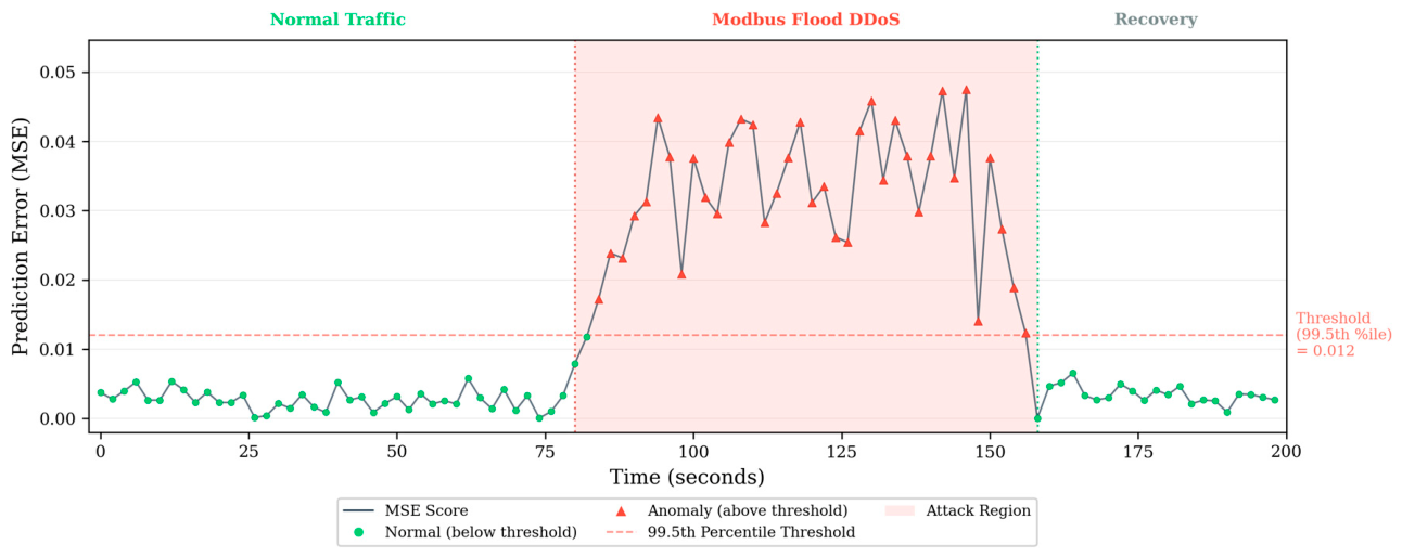
In Figure 4, we can see the illustration of a CNN-LSTM’s response to a Mod-bus flood DDoS attack. During normal traffic (first ~80 s), the prediction error remains consistently below the 99.5th percentile threshold (~0.012), fluctuating between approximately 0.002 and 0.008 (green points). When the Modbus flood begins, the score rises sharply and exceeds the threshold within a few ticks, peaking near 0.05, roughly 4× the threshold value (red triangles). After a short time, the attack cools down, and the score drops back below the threshold during the recovery phase. The clear separation between normal and attack scores, with minimal overlap near the threshold boundary, apparently confirms that the prediction-based detection approach produces well-discriminated anomaly signals for volumetric Modbus flooding.

3.4. Ablation Study

A window size of 20 ticks (40 s) provides the best balance between detection accuracy and computational cost, as illustrated in

Table 12. Window size ablation (mean ± std. across 10 folds, using 99.5th percentile threshold).

Window Size (ticks)	Precision	Recall
10	0.934 ± 0.021	0.917 ± 0.024
20 (default)	0.967 ± 0.012	0.953 ± 0.014
30	0.971 ± 0.011	0.949 ± 0.015
40	0.969 ± 0.013	0.944 ± 0.017

. Shorter windows (10 ticks) lack sufficient temporal context for the LSTM to learn stable metric trajectories, reducing both precision and recall. Larger windows (30 and 40 ticks) provide marginal precision improvements (+0.4 and +0.2 points) but reduce recall and increase processing overhead. Each window contains more timesteps, increasing inference latency.

Table 13. Threshold percentile ablation (mean ± std. across 10 folds, using window size of 20).

Percentile	Precision	Recall
90th	0.891 ± 0.023	0.978 ± 0.009
95th	0.928 ± 0.017	0.971 ± 0.011
97th	0.947 ± 0.014	0.964 ± 0.013
99th	0.961 ± 0.013	0.958 ± 0.014
99.5th (default)	0.967 ± 0.012	0.953 ± 0.014

confirms that the 99.5th percentile threshold achieves the best precision–recall balance. Lower percentiles increase recall (the 90th percentile reaches 0.978 recall) but at the cost of substantially lower precision (0.891), meaning more false alarms during normal operation.

The 99.5th-percentile threshold is a reasonable choice for production deployment, not just for the experimental study. At the 2 s tick rate, the gateway processes 43,200 windows per day (86,400/2), so a nominal 0.5% false-positive rate translates to roughly 216 isolated window-level flags per day under stationary normal traffic. In practice, the alarm load an operator actually faces is much smaller than this number, for two reasons. First, real attacks span many consecutive windows—a Modbus flood lasts 15 to 30 ticks, and an MQTT or DNP3 burst 7 to 22 ticks (Table 5)—so a genuine attack lights up a long run of consecutive windows, while false positives at the 99.5th percentile are statistically isolated single-window events; a simple “alert only after N out of M consecutive windows are flagged” rule removes almost all of them without losing real attacks and drops the effective alert rate by roughly an order of magnitude. Second, the 99.5th percentile sits at the sweet spot of the precision–recall trade-off in Table 13. Moving from the 99th to the 99.5th percentile buys only 0.6 pp of precision at the cost of 0.5 pp of recall, and tightening further gives almost no additional precision while continuing to lose recall, especially on DNP3 response flooding, which is already the hardest attack to detect and has the highest false-negative rate (Table 11); raising the threshold would save a handful of false alarms per day at the cost of letting more real DNP3 attacks slip through, the worse trade-off in this setting. Deployments with stricter alarm budgets can still recalibrate the threshold against the same training reconstruction error distribution; this is a standard deployment time tuning step.

3.5. Computational Cost Analysis

As

Table 14. Computational cost comparisons.

Model	Parameters	Model Size (MB)	Training Time/Fold	Inference Time/Window
CNN-LSTM	~243K	~1.0	~8 min	~2 ms
Isolation forest	N/A	~15	~30 s	~0.1 ms
LSTM-only	~201K	~0.8	~5 min	~1.5 ms
CNN-only	~13K	~0.05	~2 min	~0.5 ms
Autoencoder	~18K	~0.07	~3 min	~0.3 ms

Hardware: AMD Ryzen 9 5900HX (Advanced Micro Devices, Inc., Santa Clara, CA, USA), 32 GB of RAM, and CPU-only training and inference.

shows, all models achieve inference times well below the 2 s gateway sampling interval, confirming that real-time deployment is feasible without dedicated GPU hardware. The CNN-LSTM requires the most training time (~8 min per fold), but this is a one-time cost performed offline before deployment. The isolation forest is the fastest to train (~30 s per fold) and the fastest at inference (~0.1 ms per window), but as shown in Section 3.1, it provides inferior detection performance. The CNN-LSTM’s model size (~1.0 MB) is an order of magnitude smaller than the isolation forest’s serialized model (~15 MB), because tree ensembles store all split boundaries. The autoencoder baseline introduced in Section 2.3.5 sits between the CNN-only and LSTM-only ablations on almost every cost dimension: approximately 18 K parameters and ~0.07 MB on disk, ~3 min training per fold, and ~0.3 ms inference per window, well within the 2 s sampling-interval budget.

3.6. Operational Deployment Demonstration

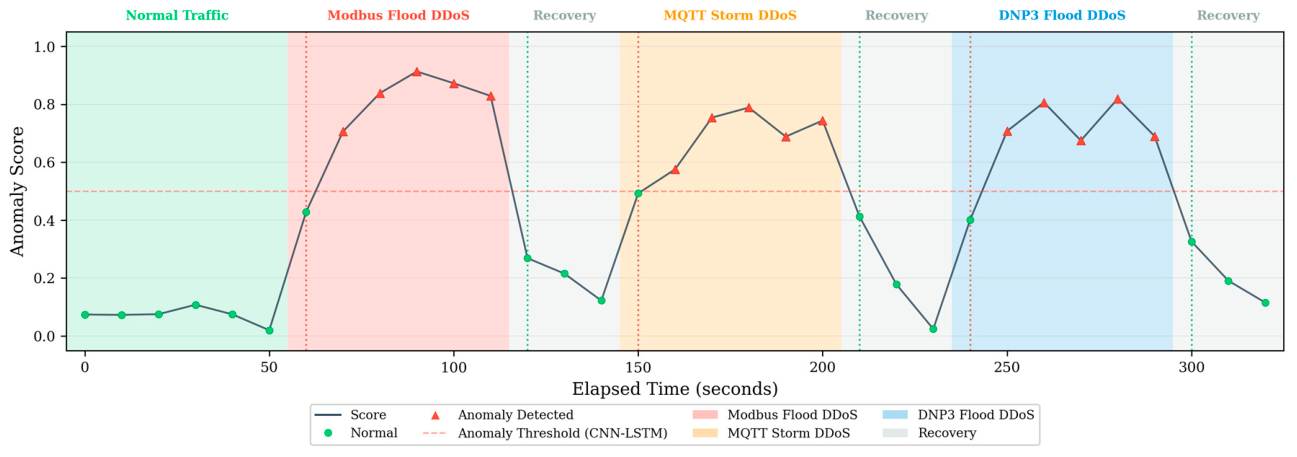
To validate that the CNN-LSTM operates correctly within the full monitoring platform, we conducted not only an offline batch evaluation but also a live operational test. The microgrid gateway simulator was started, generating normal Modbus, MQTT, and DNP3 traffic at 2 s intervals. The trained CNN-LSTM model was loaded into the Python FastAPI inference service via the model registry. Incoming traffic was ingested through the .NET backend REST API, processed by the feature engineering pipeline in real time, and passed to the CNN-LSTM for inference. After a period of normal operation, each of the three DDoS attack scenarios was triggered sequentially via the attack simulation API. The system was observed to determine whether the model correctly detected each attack in a live operational setting, with results logged as AnomalyEvent records in the PostgreSQL database.

Figure 5 demonstrates the CNN-LSTM operating within the full monitoring platform under live conditions. During the initial normal traffic period (~0–50 s), the anomaly score remained below the threshold (green points). When the Modbus flood DDoS was triggered, the score rose above the threshold within seconds (red triangles), peaking near 0.8, and an AnomalyEvent was recorded in the database. After the attack stopped, the score returned to baseline during the recovery period. The MQTT storm DDoS was then triggered, producing a similar spike with peaks near 0.75, followed by recovery. Finally, the DNP3 flood DDoS produced peaks near 0.7 before recovery. All three attack types were correctly detected in sequence, confirming that the detection model functions correctly when deployed through the complete data pipeline from the gateway simulator through .NET ingestion through Python inference to anomaly logging.

To substantiate the real-time deployment claim beyond the model-only inference time reported in Table 14, we conducted a sustained-load end-to-end latency test with the proposed CNN-LSTM as the active detection model, loaded via the FastAPI model registry. Because the CNN-LSTM has the highest per-window inference time of the five models in Table 14, this configuration represents the worst-case pipeline latency: any deployment of the lighter baselines (isolation forest, autoencoder, LSTM-only, and CNN-only) trivially satisfies the same real-time bound. The microgrid gateway simulator was driven for one continuous hour at the nominal 2 s tick rate (1800 ingestion events), and per-stage timestamps were captured along the full pipeline: HTTP send from the simulator client, .NET REST handler entry, feature-engineering completion, FastAPI inference response, and AnomalyEvent commit to PostgreSQL.

Table 15. End-to-end pipeline latency under sustained load (1 h, 1800 ingestion events at 2 s tick rate).

Stage	p50 (ms)	p95 (ms)	p99 (ms)
HTTP ingest → .NET handler entry	1.6	3.8	5.4
.NET handler → feature-engineering output	9.2	17.4	24.8
Feature-engineering output → FastAPI inference	27.5	45.2	59.7
FastAPI response → AnomalyEvent commit	6.8	12.6	19.3
End-to-end (HTTP send → DB commit)	45.9	76.3	98.4

summarizes the p50, p95, and p99 latencies—the 50th, 95th, and 99th percentiles of the measured per-event latency distribution—per stage and end-to-end.

Across 1800 ingestion events, the end-to-end p99 latency is 98.4 ms, well below the 2000 ms gateway sampling interval, with a median end-to-end latency of 45.9 ms. The dominant contribution is the feature-engineering inference stage (p99 = 59.7 ms), which includes the cross-process HTTP round-trip between the .NET backend and the Python FastAPI inference service. The PostgreSQL AnomalyEvent commit contributes p99 = 19.3 ms under sustained load, dominated by fsync latency, and could be reduced further by batched writes or async write-behind if needed at higher ingestion rates. Test platform: AMD Ryzen 9 5900HX and 32 GB of RAM; CPU utilization remained below 18% and resident memory below 1.6 GB throughout the test.

4. Conclusions

This paper proposed an unsupervised CNN-LSTM framework for detecting DDoS attacks in smart microgrid communication infrastructure. The model was trained exclusively on normal OT traffic from a simulated microgrid gateway handling Modbus TCP, MQTT, and DNP3 communication, and evaluated against three protocol-specific attack scenarios that were unseen during training. The CNN-LSTM achieved the highest precision and recall among all evaluated models, outperforming the isolation forest baseline, the autoencoder baseline, and both ablation variants on both metrics. The largest advantage appeared in DNP3 response flooding, the attack type with the subtlest traffic signature.

Due to the lack of a sufficient amount of labeled attack samples, an unsupervised approach was employed to tackle this problem using metric-rich time-series data generated by the simulated microgrid gateway environment described in Section 2.2.3. A dual-path architecture is proposed, which leverages the strengths of recurrent and convolutional structures through LSTM and CNNs, respectively. LSTM is utilized to capture temporal features from time-series, and CNNs are leveraged to extract spatial features from the flow aggregate. The experimental results reveal that removing either stream would impede performance. Notably, the performance of the LSTM-only variant is higher than that of the CNN-only variant. Extensive statistical analysis performed across 10-fold experiments demonstrates that the hybrid architecture outperforms individual baselines as well as existing unsupervised approaches.

Validation of the dual-domain monitoring architecture, in which the CNN-LSTM proposed here operates in parallel with the device-level autoencoder of our prior work [1], is positioned as a direction for future work rather than as a validated outcome of the present study. Subsequent research will design alert-fusion strategies that combine network-layer and device-layer anomaly signals into joint operator alerts and deploy both methods concurrently on a campus-microgrid testbed to evaluate joint detection coverage, false-alarm behavior under correlated benign disturbances, and operator workload.

Several limitations of the present study should be noted. First, all evaluations are conducted on traffic generated by the microgrid gateway simulator described in Section 2.2.3; the results are, therefore, preliminary and simulator-bound, and real-microgrid validation remains outstanding before operational deployment. Second, the three injected DDoS scenarios are all volumetric or sub-volumetric flood patterns; very low-intensity, slow-rate attacks designed to remain within the normal traffic envelope have not been characterized and may require complementary detection mechanisms. Third, the model is trained on a fixed normal distribution; operational deployments will encounter concept drift as microgrid behavior evolves with seasonal load and added devices, potentially producing nuisance false positives until the model is retrained. These limitations map onto the future-work avenues listed below.

Future work will explore five avenues for extending the framework: (1) stronger temporal models, for instance, transformer architectures with self-attention, that capture longer range traffic context than the present 20-tick window; (2) topology-aware detection that incorporates microgrid layout and device-role information into learned features, so that anomalies for one device class need not be anomalous for another; (3) concept-drift detection and adaptive retraining as normal traffic patterns evolve with seasonal load and added devices, with adaptive thresholding tied to a continuously estimated operational FPR budget complementing the static 99.5th-percentile threshold used in the present study; (4) expansion of the attack taxonomy to non-volumetric threats—man-in-the-middle, protocol manipulation, and slow-rate request–response attacks—which the present three-scenario evaluation does not cover; and (5) evaluation on a physical campus-microgrid testbed with real OT hardware and live traffic.

References

1. Haxhismajli, B.; Hajrizi, E.; Qehaja, B.; Guliashki, V.; Marinova, G. Enhancing Microgrid Security: Web-Based Anomaly Detection Using Autoencoder. In Proceedings of the 32nd International Conference on Systems, Signals and Image Processing (IWSSIP), Skopje, North Macedonia, 24–26 June 2025. [Google Scholar]
2. Diaba, S.Y.; Elmusrati, M. Proposed algorithm for smart grid DDoS detection based on deep learning. Neural Netw. 2023, 159, 175–184. [Google Scholar] [CrossRef] [PubMed]
3. Naqvi, S.S.A.; Li, Y.; Uzair, M. DDoS attack detection in smart grid network using reconstructive machine learning models. PeerJ Comput. Sci. 2024, 10, e1784. [Google Scholar] [CrossRef] [PubMed]
4. AlHaddad, U.; Basuhail, A.; Khemakhem, M.; Eassa, F.E.; Jambi, K. Ensemble model based on hybrid deep learning for intrusion detection in smart grid networks. Sensors 2023, 23, 7464. [Google Scholar] [CrossRef] [PubMed]
5. Hosseini Rostami, S.M.; Pourgholi, M.; Asharioun, H. Enhancing resilience of distributed DC microgrids against cyber attacks using a transformer-based Kalman filter estimator. Sci. Rep. 2025, 15, 6815. [Google Scholar] [CrossRef] [PubMed]
6. Halbouni, A.; Gunawan, T.S.; Habaebi, M.H.; Halbouni, M.; Kartiwi, M.; Ahmad, R. CNN-LSTM: Hybrid deep neural network for network intrusion detection system. IEEE Access 2022, 10, 99837–99849. [Google Scholar] [CrossRef]
7. Altunay, H.C.; Albayrak, Z. A hybrid CNN+LSTM-based intrusion detection system for industrial IoT networks. Eng. Sci. Technol. Int. J. 2023, 38, 101322. [Google Scholar] [CrossRef]
8. Abdallah, M.; Le Khac, N.A.; Jahromi, H.; Jurcut, A.D. A hybrid CNN-LSTM based approach for anomaly detection systems in SDNs. In Proceedings of the 16th International Conference on Availability, Reliability and Security (ARES), Vienna, Austria, 17–20 August 2021. [Google Scholar] [CrossRef]
9. Sinha, P.; Sahu, D.; Prakash, S.; Yang, T.; Rathore, R.S.; Pandey, V.K. A high performance hybrid LSTM CNN secure architecture for IoT environments using deep learning. Sci. Rep. 2025, 15, 9684. [Google Scholar] [CrossRef] [PubMed]
10. Alashjaee, A.M. Deep learning for network security: An Attention-CNN-LSTM model for accurate intrusion detection. Sci. Rep. 2025, 15, 21856. [Google Scholar] [CrossRef] [PubMed]
11. Choi, W.-H.; Kim, J. Unsupervised learning approach for anomaly detection in industrial control systems. Appl. Syst. Innov. 2024, 7, 18. [Google Scholar] [CrossRef]
12. Altaha, M.; Hong, S. Anomaly detection for SCADA system security based on unsupervised learning and function codes analysis in the DNP3 protocol. Electronics 2022, 11, 2184. [Google Scholar] [CrossRef]
13. Zare, F.; Mahmoudi-Nasr, P.; Yousefpour, R. A real-time network based anomaly detection in industrial control systems. Int. J. Crit. Infrastruct. Prot. 2024, 45, 100676. [Google Scholar] [CrossRef]
14. Ha, D.T.; Hoang, N.X.; Hoang, N.V.; Du, N.H.; Huong, T.T.; Tran, K.P. Explainable anomaly detection for industrial control system cybersecurity. IFAC-PapersOnLine 2022, 55, 1183–1188. [Google Scholar] [CrossRef]
15. Ghosh, T.; Bagui, S.; Bagui, S.; Kadzis, M.; Bare, J. Anomaly detection for Modbus over TCP in control systems using entropy and classification-based analysis. J. Cybersecur. Priv. 2023, 3, 895–913. [Google Scholar] [CrossRef]
16. Modbus Organization. Modbus Application Protocol Specification V1.1b3. 2012. Available online: https://www.modbus.org/file/secure/modbusprotocolspecification.pdf (accessed on 2 March 2026).
17. OASIS. MQTT Version 5.0 Standard. 2019. Available online: https://docs.oasis-open.org/mqtt/mqtt/v5.0/mqtt-v5.0.html (accessed on 2 March 2026).
18. IEEE Std 1815-2012; IEEE Standard for Electric Power Systems Communications-Distributed Network Protocol (DNP3). IEEE: Piscataway, NJ, USA, 2012.
19. Bhatia, S.; Kush, N.; Djamaludin, C.; Akande, A.J.; Foo, E. Practical Modbus Flooding Attack and Detection. In Proceedings of the Twelfth Australasian Information Security Conference (AISC 2014), Auckland, New Zealand, 20–23 January 2014; pp. 57–65. [Google Scholar]
20. Alatram, A.; Sikos, L.F.; Johnstone, M.; Szewczyk, P.; Kang, J.J. DoS/DDoS-MQTT-IoT: A dataset for evaluating intrusions in IoT networks using the MQTT protocol. Comput. Netw. 2023, 231, 109809. [Google Scholar] [CrossRef]
21. Jin, D.; Nicol, D.M.; Yan, G. An event buffer flooding attack in DNP3 controlled SCADA systems. In Proceedings of the 2011 Winter Simulation Conference (WSC), Phoenix, AZ, USA, 11–14 December 2011; pp. 2614–2626. [Google Scholar] [CrossRef]
22. Hochreiter, S.; Schmidhuber, J. Long short-term memory. Neural Comput. 1997, 9, 1735–1780. [Google Scholar] [CrossRef] [PubMed]
23. Liu, F.; Ting, K.; Zhou, Z.-H. Isolation forest. In Proceedings of the 8th IEEE International Conference on Data Mining (ICDM), Pisa, Italy, 15–19 December 2008; pp. 413–422. [Google Scholar] [CrossRef]
24. Paszke, A.; Gross, S.; Massa, F.; Lerer, A.; Bradbury, J.; Chanan, G.; Killeen, T.; Lin, Z.; Gimelshein, N.; Antiga, L.; et al. PyTorch: An imperative style, high-performance deep learning library. In Advances in Neural Information Processing Systems 32 (NeurIPS); Curran Associates: Red Hook, NY, USA, 2019. [Google Scholar]
25. Pedregosa, F.; Varoquaux, G.; Gramfort, A.; Michel, V.; Thirion, B.; Grisel, O.; Blondel, M.; Prettenhofer, P.; Weiss, R.; Dubourg, V.; et al. Scikit-learn: Machine learning in Python. J. Mach. Learn. Res. 2011, 12, 2825–2830. [Google Scholar]
Figure 1. Three-tier monitoring platform architecture showing data flow from microgrid field devices through the gateway to the .NET backend, Python FastAPI machine learning (ML) service, and React.js dashboard.
Telecom 07 00058 g001
Figure 2. Feature engineering pipeline from raw gateway data to model input. Sliding windows produce a metric tensor (20, 5) and a flow aggregate vector (10,), both Min–Max-normalized.
Telecom 07 00058 g002
Figure 3. CNN-LSTM dual-branch architecture, where the LSTM branch (left) processes the metric tensor for temporal patterns, and the CNN branch (right) processes flow aggregates for spatial patterns. Both outputs are fused and passed through dense layers to predict the next tick.
Telecom 07 00058 g003
Figure 4. CNN-LSTM prediction error (MSE) over time for a representative Modbus flood DDoS episode.
Telecom 07 00058 g004
Figure 5. Live anomaly score during the operational deployment test.
Telecom 07 00058 g005