A Node Placement Algorithm Utilizing Mobile Nodes in WSN and IoT Networks ^†

Abstract

The operation of the Internet of Things (IoT) networks and Wireless Sensor Networks (WSN) is often disrupted by a number of problems, such as path disconnections, network segmentation, node faults, and security attacks. A method that gains momentum in resolving some of those issues is the use of mobile nodes or nodes deployed by mobile robots. The use of mobile elements essentially increases the resources and the capacity of the network. In this work, we present a Node Placement Algorithm with two variations, which utilizes mobile nodes for the creation of alternative paths from source to sink. The first variation employs mobile nodes that create locally-significant alternative paths leading to the sink. The second variation employs mobile nodes that create completely individual (disjoint) paths to the sink. We then extend the local variation of the algorithm by also accounting for the energy levels of the nodes as a contributing factor regarding the creation of alternative paths. We offer both a high-level description of the concept and also detailed algorithmic solutions. The evaluation of the solutions was performed in a case study of resolving congestion in the network. Results have shown that the proposed algorithms can significantly contribute to the alleviation of the problem of congestion in IoT and WSNs and can easily be used for other types of network problems.

1. Introduction

It is a widespread belief that the Internet of Things (IoT) is an emerging technology that has the power to change our future. The promise of this technology also makes it one of the most active fields of research, covering all its aspects of performance. It is in this context that the work presented here takes place and whose objective is to improve the communications within IoT networks. In our view, the device and communications part of an IoT system is a direct descendant of Wireless Sensor Networks (WSNs) [1,2], in the sense that it is about networked, resource-constrained systems mainly focusing on low-power wireless devices. As such, many IoT networks exhibit unique characteristics but also come with some important limitations, such as energy, memory and computational power. Energy [3] is a limitation of great importance for the lifetime of wireless nodes, and, as a consequence, the whole network depends on it. The energy limitations restrict nodes’ memory and computational power.

Due to the increase in traffic demand in IoT applications, many problems arise in the network [4]. The hop-by-hop communication method from the nodes to the gateway (or sink) and the limited energy power are the main reasons for the problems. As a result, the network may suffer from energy holes or hotspots, which result in congestion and/or network partitioning. An approach for solving these problems is the use of mobile elements in the network.

Mobile elements are able to change their position in the network. Algorithms that use mobile elements normally employ two distinct tactics. The employment of mobile sink(s) or mobile nodes [5]. Mobile sinks have the ability to move around the network and collect data from nodes on the spot. The mobile sink approach mitigates the problem of network disconnection due to energy consumption. On the other hand, the employment of mobile nodes, with similar characteristics as of static nodes, assist existing nodes in performing their tasks, either by replacing energy exhausted or damaged nodes or by creating alternative paths to the sink(s). Algorithms that base their operation on mobile nodes, improve the lifetime of the network [6]. Therefore, algorithms that use mobile nodes need to take into consideration the power consumption model in use [7].

The Node Placement Algorithm retains the basic principles of MobileCC and reacts upon the occurrence of congestion. It resolves the problem by efficiently and effectively relocating mobile nodes. The main idea is that the Alternative Path Creation mechanism starts when existing congestion control algorithms fail. The algorithm consists of two variations: a dynamic node placement algorithm that solves the problem locally and a direct node placement algorithm that creates a new direct path to the sink, which consists only of mobile nodes.

The extended version of the Node Placement Algorithm, called the Energy Node Placement Algorithm, reuses the mobile relay nodes already in use in the network for resolving congestion, network disconnection, energy holes, or security attack problems occurring in the network. The basic idea of placing mobile nodes in the network to mitigate the problem to be solved is retained, and the focus is set on the energy consumption of the active mobile nodes in the network. Considering the energy levels of a mobile node can be useful in re-using it in a different area of the network or in replacing it on time before causing a new problem in the network.

A preliminary version of the Node Placement Algorithm is presented in [8], while a preliminary version of the Energy Node Placement Algorithm appeared in [9]. The current work extends the discussion and findings of these previous research works and evaluates them against multiple energy models inspired by different types of mobile robots. It presents a theoretical analysis of the algorithms, as well as a comparison of the energy models.

WSNs are descendants of the new emerging technology of the Internet of Things (IoT) [10]. An IoT-enabled WSN [1] is defined as the WSN in an IoT-based system. Each sensor node is defined as an IoT-enabled sensor node that can monitor the environment and collect real-time data. An IoT-enabled WSN consists of an end-user connected to the Internet, which is also connected to an access point. The access point is represented by the base station of the WSN where all sensor nodes are connected to. In this respect, the algorithmic mechanisms proposed in our paper can be directly applied to IoT-enabled WSNs.

The contributions of the current work are the following: (a) we are the first to propose a solution that utilizes mobile nodes as alternative paths in order to unload the flows of the affected area in the network, (b) introduce a time-efficient solution for decreasing the correspondence time upon detecting a network problem, (c) consider the energy consumption of the mobile node prolonging its lifetime, and (d) evaluate different energy models of the mobile node to determine the most striving energy factor.

The paper is organized as follows. In Section 2, we present related work. In Section 3, we provide an overview of the MobileCC Framework, of which our proposed algorithms are part of. Then, in Section 4, we present the Node Placement algorithm, with its two variations, Dynamic (Section 4.1) and Direct Path (Section 4.2), and in Section 5, we present an energy-efficient extension of the Dynamic variation of the Node Placement algorithm, called the Energy Node Placement algorithm. In Section 6, the evaluation of the proposed algorithms is presented. The evaluation is divided into three parts. In the first part, the Node Placement algorithm, including both variations, is compared with a congestion control algorithm (Section 6.3.1). In the second and third parts, the Energy Node Placement algorithm is evaluated in different reuse scenarios (Section 6.3.2) and under different energy consumption models (Section 6.3.3), respectively. We conclude with a discussion in Section 7.

2. Related Work

Pang et al. [11] proposed a data collection algorithm that uses multiple mobile nodes as sink nodes. The main goal is to optimize the path planning procedure. The algorithm starts with a dynamic clustering algorithm that randomly arranges the nodes into clusters. The node with the highest energy is selected to be the cluster head that establishes the data collection cluster. Based on the number of the mobile nodes, the monitoring area is divided into several parts, and each mobile node is assigned to the respective areas to perform the data collection. The authors propose a path-based path equalization algorithm (PEABR) to adjust the path of the mobile nodes in order to optimize the path planning scheme. The proposed algorithm was simulated and analyzed in Matlab and then further analyzed in the laboratory environment to verify its reliability. The results and analysis demonstrated that the algorithm is feasible and effective.

Zhang et al. [12] presented a centralized energy-efficient clustering routing (CEECR) protocol for mobile nodes. The main goal is to minimize the energy dissipation, as well as to maximize the packet delivery ratio. The algorithm consists of two steps. In the first step, the cluster head is selected periodically based on the average energy and speed of the nodes. The ability of some nodes to move around the network makes it possible for them to get disconnected from their cluster head; these nodes are called detached nodes. As a result, the second step is about these detached nodes, which will join their optimal clusters based on multiple factors. The proposed algorithm was simulated in NS-2, and it was compared to six clustering-based protocols, LEACH [13], LEACH-C [13], LEACH-Mobile [14], CBR [15], MBR [16], and LEACH-MF [17]. The results suggest that CEECR outperforms the other algorithms in terms of energy consumption and packet delivery ratio.

To the best of our knowledge, there are no other algorithms in the literature that solve the problem of congestion using an approach as ours. The work in [11,12] use mobile nodes for routing and data collection and not to resolve any network communication problems. In a recent survey [5], the solutions utilizing mobile nodes follow two approaches. In the first approach, the mobile nodes either refer to mobile sink nodes that collect data from sensor nodes, or they are used for routing purposes. In the second one, mobile nodes are represented as mobile robots that move in the network, replacing and assisting nodes. Our work focuses only on mobile nodes, which take up the role of the sensor nodes within the network; they are not used as mobile sink nodes and are not considered as mobile robots.

3. The MobileCC Framework

The concept of utilizing mobile nodes in the network for the creation of alternative paths to the sink was initially suggested by Koutroullos et al. in [6]. The authors proposed a mechanism called Mobile Congestion Control (MobileCC), which was used in certain areas of a network that suffer from congestion repeatedly, permanently or for a long duration. The main idea of the mechanism is to create hard alternative disjoint paths only consisting of mobile nodes to resolve congestion problems that occur in the network. The initial position of the mobile nodes is alongside the sink node. They are in sleep mode and are only moved when notified from the sink to help in a congested area. This work shows that it is possible to mitigate the effects of congestion by using mobile nodes and create disjoint paths. However, the actual mobile node placement strategy is not addressed.

The network consists of randomly deployed static nodes and a set of mobile nodes placed near the sink in sleep mode. The following assumptions are also considered:

• All nodes, both static and mobile, have the same characteristics, such as computation power, communication capabilities, sensing, and transmission range, with the exception of the mobility characteristic of the mobile nodes.
• A simple MAC protocol, such as CSMA/CA, is employed.
• All nodes are aware of their absolute or relative (to the sink) location.
• The sink is informed by the nodes about their location and communication range.

The primary objective of this work is to utilize the extra resources (mobiles nodes) efficiently and effectively in order to resolve any problems in the network and, if possible, to improve its performance in terms of delay, energy efficiency and throughput. The problem has two aspects. The first aspect is the placement of the mobile nodes in such a way as to create a disjoint path made up entirely of mobile nodes to the sink, while in the other case, the mobile node creates a local disjoint path that connects with the original routes.

The framework consists of the following mechanisms (see Figure 1):

• Problem Detection Mechanism
• Defective Node Selection Mechanism
• Problem Notification Mechanism
• Alternative Path Creation Mechanism Using Mobile Nodes

  -

  Calculation of Extra Resources

  -

  Calculation of Optimum Position of Extra Nodes

  -

  Establishment of Alternative Path

Concerning the three first mechanisms, a lot of work has already been done so far in the literature. The existing detection mechanisms can be used based on the problem that occurred in the network, such as congestion [18] or failure [19]. Therefore, in this work, we focus on devising mechanisms for creating alternative paths using mobile nodes. We begin with the Node Placement algorithm, presented in the next section.

4. The Node Placement Algorithm

When a node detects a problem, it sends a Problem Notification Message (PNM) to the sink. This message contains all the information needed so that the sink can act TO mitigate the problem that appeared in the network. This information includes: its NodeID, its location and communication range, the number of packets received and forwarded per sample time period, and some neighbor table information. From the neighbor table, the following information is included: neighbor node’s NodeID, hop number, number of packets received, and availability flag.

When the sink node receives the PNM message, it calculates the position for mitigating the problem. This position needs to be a “clever” placement for a mobile node in order to provide alternative paths to the sink and help in alleviating the area from its problem. After the calculation of the position, the sink node sends a Moving Notification Message (MNM) to the mobile node that is selected to assist in the problem. The MNM message includes information about the target location, the sender node’s NodeID, and its next-hop NodeID.

When a mobile node receives an MNM message, it switches off its radio while moving towards the target location and switches its radio back on at its new position. The use of the ON/OFF tactic is so that the mobile nodes are not detectable from the static nodes in the network while they travel towards their target locations. Finally, when the mobile node reaches its destination, it establishes a connection with its target nodes to be served.

In this section we present the Node Placement Algorithms (NPA) that consists of two variations. These algorithms are described below and can be used for determining the number and position of mobile nodes.

4.1. Dynamic Node Placement (Locally-Significant Paths)

The first algorithm proposed is the Dynamic Node Placement algorithm, referred to as Dynamic MobileCC. This algorithm places a mobile node in a carefully computed position so to alleviate the problematic area and assist the affected nodes. This mobile node can forward the packets either directly to the sink if the sink is in its transmission range, or it can serve as a relay node and forward the received packets to other upstream nodes.

High-level idea. Initially, the Dynamic MobileCC algorithm calculates the average number of packets per time unit that the defective node receives and cannot forward due to lack of buffer space. Then, it discovers the nodes that transmit their packets to the defective nodes and calculates the best position that the mobile node(s) should move to in order to receive data from a number of them. Ideally, the best position is the position where the minimum number of nodes can divert their traffic through the mobile node(s), whereas at the same time, their total sending rate should be equally or more than the amount of the excess traffic of the defective node (see Algorithm 1 and Appendix A.1)).

Its operation is based on the following functions:

• Identification of defective and “defecting” nodes;
• Calculation of extra resources;
• Calculation of the position that the mobile node should be placed.

We now provide a detailed description of these functions below.

4.1.1. Identification of Defective and “Defecting” Nodes

The identification of the node that is defective and the nodes that defect this node is the first step of the algorithm. This operation is normally performed by existing detection algorithms based on the problem to be solved. This information, along with the position of these nodes, is communicated to the sink.

Algorithm 1 The Dynamic MobileCC Algorithm

1: functionDynamicMobileCCAlgorithm 2:     for all $n_j\in downNodes$ do 3:         // find the downstream nodes that have a higher receiving rate than AR 4:         if $numR>AR$ then 5:            add $n_j\in defNeighbors$ 6:         end if 7:     end for 8:     if list_length($defNeighbors$) == 1 then 9:         // find the intersection point from the line that starts from the sink and ends to node $n_j$ with the circle created from the range of the node $n_j$ 10:         p = intersectionPofL&C($n_j$,sink) 11:     else 12:         for all $n_j\in defNeighbors$ do 13:            p = intersectionPofL&C($n_j$,sink) // calculate the distance between two points 14:            dist = distance2P(p,sink) 15:            add $dist\in DistanceTable$ // create the distance list 16:         end for 17:         // find the point with the smallest distance to the sink from the Distance List 18:         p = getBestPosition($DistanceTable$) 19:     end if 20:     // determine if the point is in range of an active node 21:     flagyes = checkInRangeNode(p) 22:     if flagyes == TRUE then 23:         maddr = selectMobileNodetoUse() 24:         send newPosition(p) message to $maddr$ 25:     else 26:         set second_priority = p 27:         set flagsp = TRUE 28:     end if 29:     if flagyes == FALSE then 30:         set n = 2 31:         while $n\le 7\&\&n\le list\_length\left(downNodes\right)$ do 32:            if $n==2$ then 33:                set i = 0 34:                // find a group of two nodes that will get assist from the mobile node 35:                for all $n_i\in downNodes$ do 36:                    for all $n_j\in downNodes$ do 37:                        totalAR = ar_$n_i$ + ar_$n_j$ 38:                        if $totalAR\ge AR$ then // find the intersection point from the two circles created from the range of each nodes 39:                           p = intersectionPof2C($n_i$,$n_j$) 40:                           dist = distance2P(p,sink) 41:                           add $dist\in DistanceTable$ 42:                           i = i + 1 43:                        end if 44:                    end for 45:                end for 46:                if i > 0 then 47:                    pos = getBestPosition($DistanceTable$) 48:                    flagyes1 = checkInRangeNode($pos$) 49:                    if flagyes1 == true then 50:                        maddr = selectMobileNodetoUse() 51:                        send newPosition(pos) message to $maddr$ 52:                    else 53:                        second_priority1 = pos 54:                        flagsp1 = true 55:                        n++ 56:                    end if 57:                end if 58:            else 59:                // find a group of more than two nodes that will get assist from the mobile node 60:                for all $n_i\in downNodes$ do 61:                    for all $n_j\in downNodes$ do 62:                        p = intersectionPofL&C($n_i$,$n_j$) 63:                        for all $n_z\in downNodes$ do 64:                           totalAR = ar_$n_i$ + ar_$n_j$ + ar_$n_z$ 65:                           if $totalAR\ge AR$ then 66:                               isRange = checkIsRange($p,n_z$) 67:                               if isRange == TRUE then 68:                                   count = count + 1 69:                               end if 70:                           end if 71:                        end for 72:                        if count == $n-2$ then 73:                           dist = distance2P(p,sink) 74:                           add $dist\in DistanceTable$ 75:                        end if 76:                    end for 77:                end for 78:                pos = getBestPosition($DistanceTable$) 79:                flagyes1 = checkInRangeNode($pos$) 80:                if flagyes1 == TRUE then 81:                    maddr = selectMobileNodetoUse() 82:                    send newPosition(pos) message to $maddr$ 83:                else 84:                    distp = distnace2P(pos,sink) 85:                    distp1 = distnace2P(second_priority,sink) 86:                    if $distp\le distp1$ then 87:                        second_priority1 = pos 88:                        flagsp1 = true 89:                    end if 90:                end if 91:            end if 92:         end while 93:     end if 94:     if flagsp1 == FALSE && flagsp == TRUE then 95:         maddr = selectMobileNodetoUse() 96:         send newPosition(second_priority) message to $maddr$ 97:     else if flagsp1 == TRUE && flagsp == FALSE then 98:         maddr = selectMobileNodetoUse() 99:         send newPosition(second_priority1) message to $maddr$ 100:     else 101:         distp = distnace2P(second_priority,sink) 102:         distp1 = distnace2P(second_priority1,sink) 103:         if $distp\le distp1$ then 104:            maddr = selectMobileNodetoUse() 105:            send newPosition(second_priority) message to $maddr$ 106:         else 107:            maddr = selectMobileNodetoUse() 108:            send newPosition(second_priority1) message to $maddr$ 109:         end if 110:     end if 111: end function

4.1.2. Calculation of Extra Resources

In this step, the Additional Resources are calculated based on the average number of packets per time unit (seconds) that the defective node receives and is not able to forward. This parameter defines the excess traffic the mobile node will require to accommodate. In particular, for a defective node i, the $AdditionalResources$ rate $AR\left(i\right)$ is calculated by the equation:

$$AR\left(i\right)=\frac{Recv\left(i\right)-Tran\left(i\right)}{t-t_0}$$

(1)

where

• $Recv\left(i\right)$ is the number of packets that i has received from its neighbors,
• $Tran\left(i\right)$ is the number of packets that i has transmitted,
• t is the current time, and
• $t_0$ is the time that i started transmitting packets.

Based on this equation, the mobile node that will move close to the problematic area should be able to receive and forward the excess traffic load that cannot be forwarded by the defective node. Thus, the defective node will receive just the traffic it can accommodate, and the problem will be alleviated.

Below a more detailed description of each step is presented.

4.1.3. Calculation of the Position That the Mobile Node Should Move to

The algorithm checks whether there is a single node, which if it stops transmitting towards the defective node, the problem will be alleviated. If there is such a node, then the single point where the mobile node should move to is calculated (Algorithm 1, lines 8–10). Otherwise, if there is more than one node, then for each of these nodes, a specific point is calculated. The objective of this algorithm is to minimize the number of nodes that will transmit data through the mobile nodes, but their total sending rate should be equal to the amount of traffic that the defective node is not able to forward (Algorithm 1, lines 11–15). Furthermore, the mobile nodes should be placed in a position where at least an upper non-defective node should exist in their transmission range to forward the data they receive to the sink (Algorithm 1, lines 17–19).

Finding the position where mobile nodes should move in order to serve one node. The calculation of this specific point is performed as follows: Initially, the intersection points between the circle that are created by the radius of the transmitting range of the defective node and the straight line that connects the sink with this node are calculated (function intersectionPofL&C). Between these two points, the point that is closer to the destination node in comparison to the point that is closer to the mobile node is chosen. This is illustrated in Figure 2a.

Let us consider $(X_k,Y_k)$ as the coordinates of the node that is going to be served by the mobile node and $(X_{sink},Y_{sink})$ the coordinates of the sink. In the case that the coordinate X of this node or Y respectively, is the same as of sink’s, i.e., if $X_k=X_{sink}$, then the intersection point will be $(X_k,Y_k+nod{e}^{\prime }sTxrange)$ if $Y_k<Y_{sink}$ and $(X_k,Y_k-nod{e}^{\prime }sTxrange)$ if $Y_k<Y_{sink}$. If $Y_k=Y_{sink}$, then the intersection point will be $(X_k-nod{e}^{\prime }sTxrange,Y_k)$ if $X_k>X_{sink}$ and $(X_k+nod{e}^{\prime }sTxrange,Y_k)$ if $X_k<X_{sink}$.

For each node that has a sending rate greater than the $AdditionalResources$ rate, the position of the mobile node is calculated and the algorithm checks whether there is a node closer to the sink that is not defective so as to transmit the data that it receives.

Finding the position where mobile nodes should move in order to serve more than one node. If there is not an available relocation position for the mobile node suitable to serve just one node, then for a number of nodes equal to n (Algorithm 1, lines 26–81), where n is a number between 2 and 6 according to [20,21], the following procedure is followed:

Initially, the algorithm described in [22] is employed. This algorithm identifies the subset of the nodes that transmit their data to the defective node. Only the subsets that have a total sending rate greater than the $AdditionalResources$ rate of the defective node are used for calculations (Algorithm 1, lines 30–47 and 48–81). For each of these subsets, the algorithm finds the common point in the transmission range of the nodes, which is closer to the sink. To achieve this, the algorithm considers, for each pair of these nodes, the cross-section of their transmitting ranges. Then, it checks whether this cross-section point is within the transmitting range of the rest of the nodes, besides the pair under reference (Algorithm 1, lines 48–65). If for a subset of nodes, more than one appropriate point is calculated, then the point that is closer to the sink is chosen (Algorithm 1, lines 66–81). This is illustrated in Figure 2b.

The procedure halts when at least a common subset of nodes n is found, for $n\in [2,6]$. If there is more than one subset of size n, and more than one common point, then a mobile node is chosen to move to the common point that is closer to the sink. Thus, the algorithm makes sure that, from the smallest subset ($n=2$) to the largest subset ($n=6$), the subset that is being served by the mobile node is the smallest. This attribute secures the validity of the first limitation of this algorithm, that the least number of nodes should change the destination.

4.2. Direct Node Placement Algorithm

The second algorithm proposed is the Direct Node Placement algorithm, referred to as Direct MobileCC. Similar to the Dynamic MobileCC algorithm, it does not replace any existing topology control, congestion control, or routing algorithms but runs alongside them. The difference between the two algorithms relies on the use of the mobile nodes. While the Dynamic MobileCC uses a mobile node for each problem occurrence, the solution is local; the Direct MobileCC creates a completely new and direct (disjoint) alternative path of mobile nodes towards the sink. This solution provides a faster establishment of the connection to the sink node. As our experimental evaluation shows (cf., Section 6.3.1), this helps to reduce the number of dropped packages, trading, however, use of resources (and hence, energy).

Initially, the Direct MobileCC algorithm calculates the position of the first mobile node placed in the network with the use of the Dynamic MobileCC algorithm. Then, a direct line is created that starts from the first placed mobile node and ends at the sink. This line is filled with additional mobile nodes until a direct connection with the sink is achieved (see Algorithm 2 and Appendix A.2).

Its operation is based on the following functions:

• Calculation of the position of the first mobile node using the Dynamic MobileCC algorithm.
• Creation of a path consisting of mobile nodes, starting from the first mobile node that was placed from the previous function and ending at the sink.

Algorithm 2 The Direct Path MobileCC Algorithm

1: functionDirectPathMobileCCAlgorithm 2:     // to calculate the new position of the mobile node call the dynamic algorithm 3:     pos = DynamicMobileCCAlgorithm() 4:     flagdp = false // a flag to stop the loop 5:     while flagdp == false do 6:         // to determine if the position is in the range of the sink 7:         isSinkRange = checkinrangeofsink(pos,sink,Range) 8:         if isSinkRange == true then 9:            // to select the mobile node that is available to be sent to position pos 10:            call send_mnode(pos) 11:            flagdp = true; 12:         else 13:            // to select the mobile node that is available to be sent to position pos 14:            call send_mnode(pos) 15:            // find the interesection point from the line at pos and the circle of the sink 16:            pos = intersectionPofL&C(pos,sink,Range) 17:         end if 18:     end while 19: end function

4.2.1. Calculation of the Position of the First Mobile Node

The first mobile node is located at the position calculated by using the Dynamic MobileCC Algorithm 1. If this mobile node is in the range of the sink and is able to transmit its received data directly to it, the process terminates. Otherwise, the process continues with the following step.

4.2.2. Creation of a Path Consisting of Mobile Nodes

In order to reach the sink node, it is needed to create a disjoint path. Each new mobile node placement is calculated from the algorithm so that it is in the range of the previously placed mobile node. The calculation of this specific point is performed as follows: The intersection points of the virtual circles created by the transmitting range of the initially placed mobile node and the virtual straight line between this node to the sink is calculated. The point that is closer to the sink is the one kept. This is illustrated in Figure 2c. The process continues until the mobile node is in the sink.

5. The Energy Node Placement Algorithm

The previous algorithm stops when the mobile node is placed in the needed position and becomes active. However, at some point, the current problem may be resolved, and the mobile node may no longer be needed. For this reason, we extended the previously mentioned algorithm (the Dynamic variation) in order to reuse the mobile nodes that are placed in the network. We call this extension Energy Node Placement algorithm (eNPA), and we refer to it as Dynamic MobileCC+. In this respect, we introduce energy considerations. Based on the energy levels of the mobile nodes, they can be either be reused or be replaced; in the latter, the mobile node returns to its initial position (near the sink) to recharge its battery.

When a new problem occurs in the network, there is a need to use a mobile node to resolve it. The introduction of reuse provides the opportunity to first check among the in-use mobile nodes, that is, the mobile nodes that are already placed in the network, whether one of them is available to be used. The following conditions must be applied to reuse an in-use mobile node:

1.

The current problem for which the mobile node was sent to resolve has now been resolved, or the neighbor nodes of the mobile node can now find an alternative path.

2.

The energy level of the mobile node does not exceed a certain threshold, which enables the mobile node to travel from its current position to the new position, and then from there to its initial position (near the sink) without running out of energy.

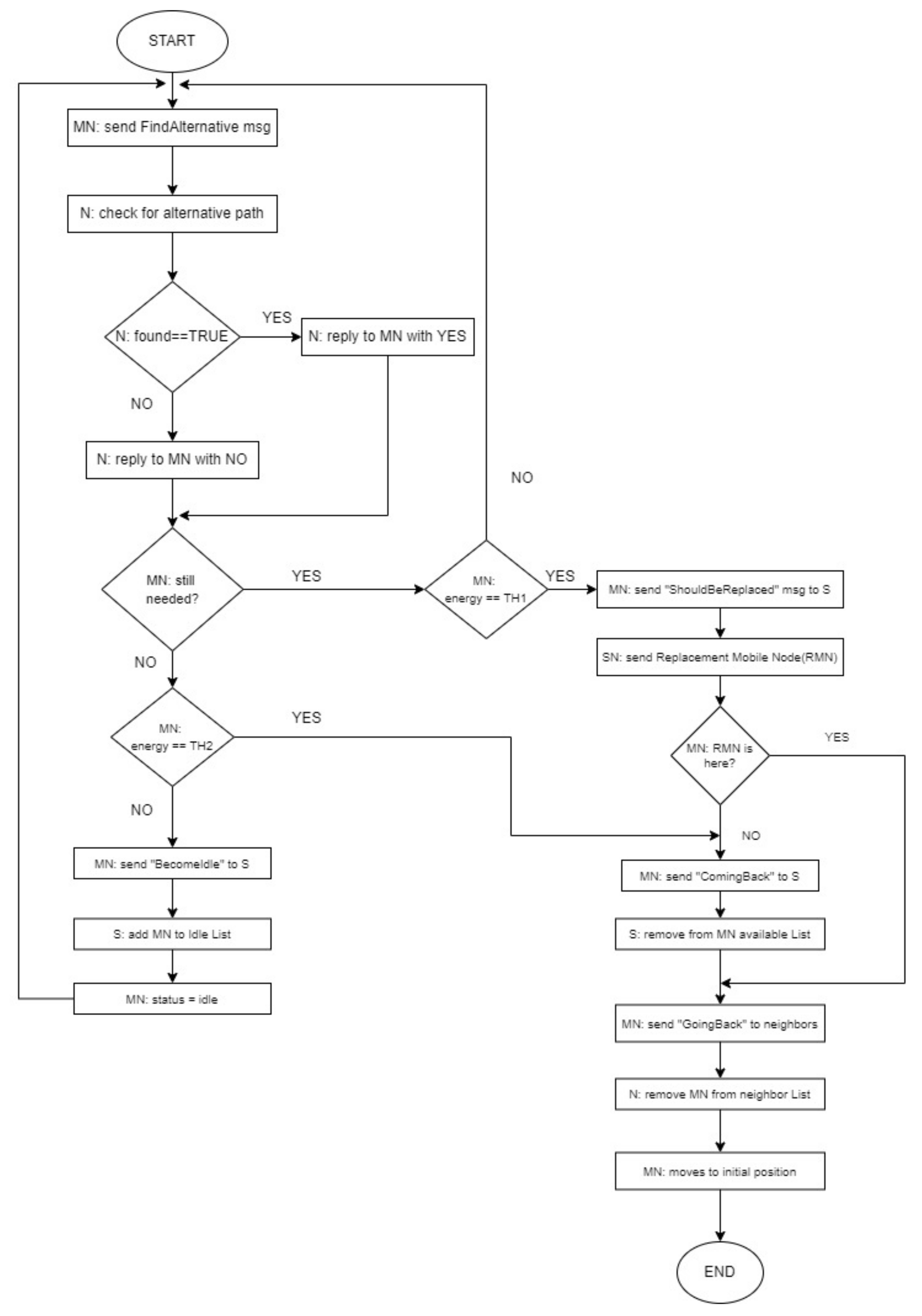
We now present the actions of each node type: Mobile node, Sink node, and node (a static node or an in-use node acting as a relay). In Appendix A.3 you can find the flowchart of this algorithm.

5.1. Mobile Node

The mobile nodes are responsible for monitoring their energy and their usage in the network. This monitoring process is performed with the use of two functions: (a) the network usage function (see Algorithm 3), which is called periodically, and (b) the energy usage function (see Algorithm 4), which works as a push notification function.

Algorithm 3 Check Usable Function for mobile node $m_i$

1: functioncheck_usable 2:     send(FindAlternative) to each $n_j\in DN$ 3:     wait until all $n_j\in DN$ to reply 4:     if $\exists repl{y}_j==\mathit{FA}-\mathit{SearchFailed}$ then         5:         broadcast(SearchFail)         6:         return $FALSE$ // $m_i$ needed 7:     end if 7: return$TRUE$ // $m_i$ not needed 8: end function

Algorithm 4 Energy Usable Function for mobile node $m_i$

1: functionenergy_usable 2:     remain_energy = listening_energy + moving_energy 3:     return_energy = the energy needed to return to its initial position. 4:     double_return_energy = double the amount of return_energy. 5:     if $remain\_energy==double\_return\_energy$ then 5:         return $TH1$ // energy reached threshold 1 6:     else if $remain\_energy==return\_energy$ then 6:         return $TH2$ // energy reached threshold 2 7:     else 7:         return $OK$ // energy is ok 8:     end if 9: end function

The procedure starts by calling the two usage functions (Algorithm 6, lines 1–2). Based on their outcome, the mobile node decides its next action, as described below:

• When the node is still needed, and its energy level is OK, the mobile node continues to act as a static node (Algorithm 6, lines 3–5).
• When the node is not needed, and its energy level is OK, the mobile node changes its status to idle and informs the sink node with a BecomeIdle message, as well as its neighbors, about its new status. (Algorithm 6, lines 6–10).
• When the node is needed, but its energy level has reached the first threshold (warning threshold), the replacement procedure is triggered: the mobile node requests from the sink a replacement and waits until either the timer (Treplaced) expires or its energy level reaches the second threshold (departure threshold). When the timer expires, which determines a time interval in which the sink node needs to send a replacement, the node informs its neighbors about its departure and leaves (by this time, a replacing node should have arrived). However, when the second energy threshold is reached, the mobile node informs the sink node and its neighbors about its departure, and then it returns to its initial position (at the sink) to get recharged (Algorithm 5, lines 11–23).
• When the node’s energy level reaches the second threshold, and the node is not needed (possibly it is idle), it will inform the sink node and its neighbors about its return and move back to its initial position (Algorithm 6, lines 24–28).

Algorithm 5 Periodic check algorithm for mobile node $m_i$

1: flag_nu = network_usable() 2: flag_eu = energy_usable() 3: if flag_nu == FALSE AND flag_eu == OK then         4:     do nothing 5: end if 6: if flag_nu == TRUE AND flag_eu == OK then         7:     status = idle         8:     send(BecomeIdle) to sink         9:     send(Idle) to to each $n_j\in neighbor\_list$ 10: end if 11: if flag_nu == FALSE AND flag_eu == TH1 then         12:     send(ShouldBeReplaced) to sink         13:     wait until Treplace OR remain_energy == TH2         14:     if remain_energy == TH2 then                15:         send(ComingBack) to sink                16:         send(GoingBack) to each $n_j\in neighbor\_list$                17:         move to init_pos 18:     end if        19:     if Treplace expired then                20:         send(GoingBack) to each $n_j\in neighbor\_list$                21:         move to init_pos 22:     end if 23: end if 24: if flag_nu == TRUE AND flag_eu == TH2 then         25:     send(ComingBack) to sink         26:     send(GoingBack) to each $n_j\in neighbor\_list$         27:     move to init_pos 28: end if 29: upon receive (“NewPosition”) from sink then 30: move to new_pos

5.1.1. Network Usage Function

This function checks whether the mobile node is still needed for the specific problem occurrence. Algorithm 4 describes this function.

The procedure starts with a (FindAlternative) request to each downstream node (DN). This request requires a DN to search its neighbor table in order to find an alternative node to send its packets. The procedure stops when at least one DN replies with a FA-SearchFail message. The mobile node broadcasts a SearchFail message, and the function returns a False value, which means it is still needed. However, when all replies are Successful messages, the mobile node is no longer needed, and the function returns a TRUE value.

5.1.2. Energy Usage Function

This function retrieves the current energy level of the mobile node at any time. Algorithm 5 describes this function.

The function starts by calculating three parameters: the remaining energy, the return_energy, and the double_return_energy. The remaining energy is defined as the sum of the listening and moving energy of the node (more info can be found in Section 6.3.2). The return_energy is defined as the energy needed from the mobile node to return to its initial position (at the sink), whereas the double_return_energy is defined as double the amount of the return_energy (to give enough time for the replacing node to arrive). The level of the remaining energy of the mobile node defines the energy threshold returned from this function. When the energy level equals the double_return_energy, the function returns TH1, which means that the first energy threshold is triggered. When the energy level drops to the return_energy, the function returns TH2, which means that the second energy threshold is triggered. Otherwise, the energy level of the mobile node is normal, and the function returns OK.

5.2. Sink Node

In Dynamic MobileCC, the sink node was only responsible for assigning an idle mobile node (of those waiting near the sink) for each problem occurrence in the network. In our extended version, the sink node may choose either an idle mobile node that resides at the sink ($MList$) or one that is already placed in the network for a previous problem ($idleMList$), if one exists. Algorithm 6 describes the tasks of the sink node.

Algorithm 6 Algorithm for sink node

1: functionsend_mnode($new\_pos$) 2:     if $idleMList==empty$ then 3:         choose $m_k\in MList$ 4:         send(NewPosition) to $m_k$ 5:     else 6:         $distnac{e}_m$ = distance(sink_pos, new_pos) 7:         $distanc{e}_i$ = distance($closestIM\_pos$,new_pos) 8:         if $distnac{e}_m<distanc{e}_i$ then 9:            choose $m_k\in idleMList$ 10:         else 11:            $m_k=closestIM$ 12:         end if 13:         send(NewPosition) to $m_k$ 14:     end if 15: end function 16: upon receive (“problem_notification”) from $n_i$ then 17: new_pos = DynamicMobileCCAlgorithm() 18: call send_mnode(new_pos) 19: upon receive (“ShouldBeReplaced”) from $m_i$ then 20: $new\_pos=currentpositionof{m}_i$ 21: call send_mnode(current position of $m\_i$) 22: upon receive (“ComingBack”) from $m_i$ then 23: if$m_i\in idleMList$then 24:     remove $m_i$ from idleMList 25: end if 26: $fla{g}_{m_i}$ = $FALSE$ 27: $current\_po{s}_{m_i}=init\_po{s}_{m_i}$ 28: upon receive (“BecomeIdle”) from $m_i$ then 29: $statu{s}_{m_i}=idle$ 30: add$m_i\in idleMList$

The selection of which mobile node to send is made on the closest distance to the calculated position. Initially, the sink defines the closest idle mobile node ($closestIM$) based on its distance ($distanc{e}_i$). Then, $distanc{e}_i$ is compared to the distance of a near sink mobile node ($distanc{e}_m$). The mobile node with the smallest distance is sent to the calculated position (see Algorithm 6, lines 1–15).

Another task of the sink node is to replace an in-use mobile node in the case of an energy emergency. When a mobile node informs the sink about the need of replacement, the sink node assigns the position to a new idle mobile node by choosing the closest idle mobile node in the network (see Algorithm 7, lines 19–21). Additionally, the sink node needs to keep track of the current status of the in-used mobile nodes. In this respect, notification messages received by the mobile nodes must be processed by the sink node. When a mobile node is about to return to its initial position, the sink node is informed in order to change its availability ($fla{g}_{m_i}$), its position, and, if necessary, remove it from the idle list (see Algorithm 7, lines 22–27). When a mobile node is not needed and becomes idle at its current position, the sink node is informed and changes the status of the mobile node, and it is added to the idle list (see Algorithm 7, lines 28–30).

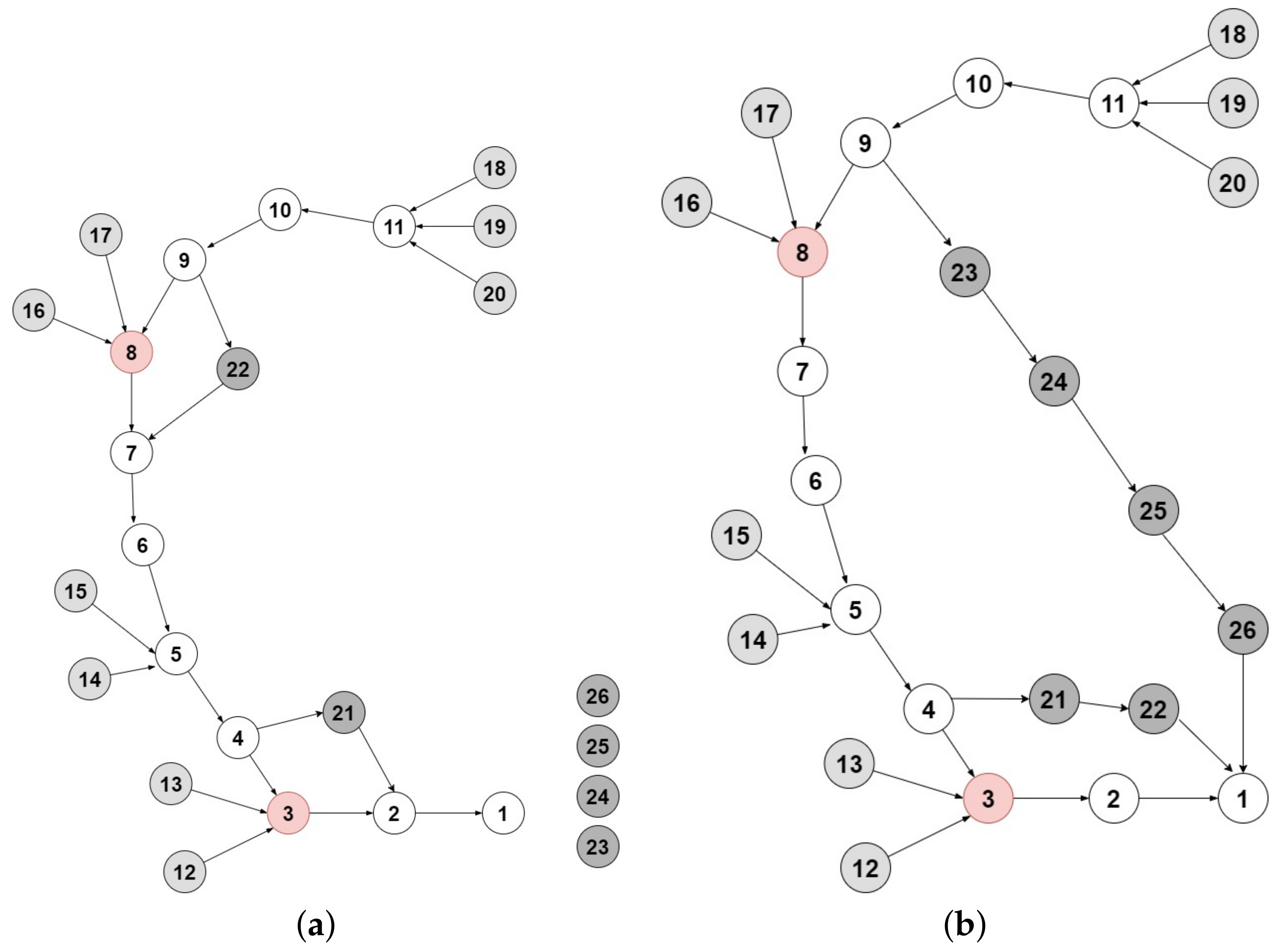
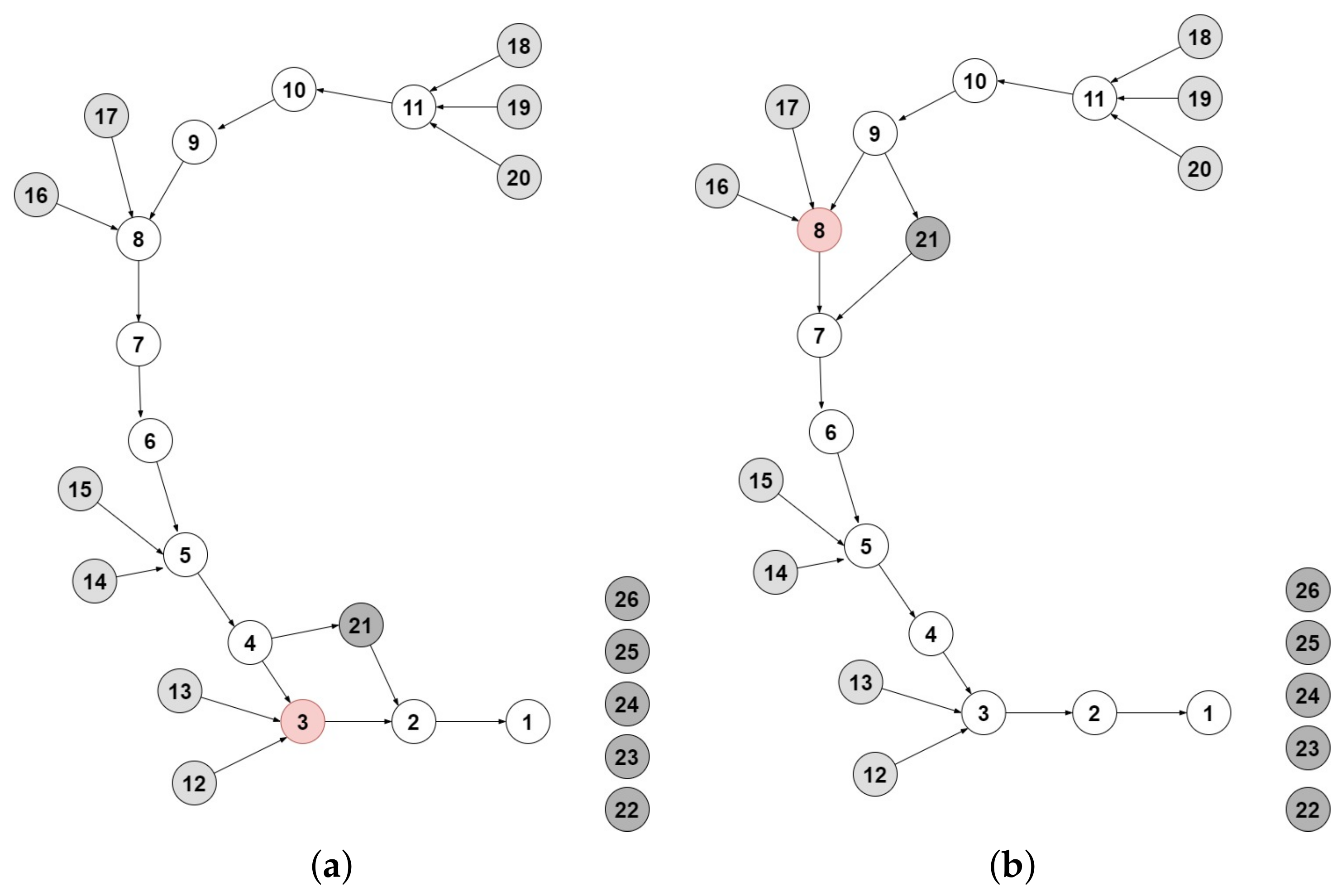
We proceed to a simple analysis of the sink node algorithm, depending on whether there is reuse or not. Specifically, when a new problem occurs in the network, the computational delay (defined below) for the whole process is divided into two cases based on the scenario used, the no reuse scenario and the reuse scenario.

No Reuse Scenario(Figure 3a): The notification information is sent (link a) from node “N” to the sink “S” and then a moving notification is sent (link b) from “S” to a near-sink mobile node “MN”. “MN” moves (link c) to its new position “X”.

Reuse Scenario(Figure 3b): The notification information is sent (link a) from node “N” to the sink “S” and then a reuse notification is sent (link b) from “S” to an in-used mobile node “MN” in the network. “MN” moves (link c) from its current position in the network to its new position “X”.

As a result, we can define the total computational delay or delay for short, as the sum of the communication delay (links a and b) and the moving delay (link c), i.e.,

$$delay=communication\_delay+moving\_delay.$$

The $communication\_delay$ is calculated as $r*dist\_hops$, where r is the rate of the packet per hop and $dist\_hops$ is the distance in hops, from the problematic area (N) to the sink (S) and from the sink to the mobile node (MN). For the no reuse case, in the worst case, $dist\_hops=D$, where D is the diameter of the network (and b is almost zero), whereas, for the reuse case, in the worst case, $dist\_hops=2D$; however, the closer the in-use mobile node is to the problematic area, the smaller the moving delay will be.

The $moving\_delay$ is calculated as $speed*distance$, where $speed$ is the speed of the mobile node and $distance$ is the distance the mobile node must move from its current position to its new position. As the algorithm attempts to find the mobile node that is closer to the position to be moved (X), which could be a mobile node at the sink or an in-use mobile node and given that in general, the moving delay is longer than the communication delay (unless an auxiliary device is used to move the mobile node, e.g., a drone), the algorithm using reuse can significantly reduce the moving delay, and hence the total delay (cf. Section 6.3.2).

5.3. Node

The role of a node in the network is performed by either a static node or an in-use mobile node acting as a relay node. In this extended version, the node is not only responsible for forwarding the packets it receives, but it also needs to respond to requests from the mobile node in its neighborhood, which defines the search process.

A search process begins upon receiving a usage request from a neighboring mobile node (see Algorithm 7, lines 1–2). The goal of this method is to search the neighboring table in order to find an alternative path excluding the mobile node. Two different methods are implemented (called at line 2 of Algorithm 7): the optimistic method (see Algorithm 8) and the allocation method (see Algorithm 9), described below. Algorithm 7 shows all tasks of a static node.

Algorithm 7 Algorithm for node $n_i$

1: upon receive (“FindAlternative”) from $m_j$ then 2:         call optimistic_method() OR allocation_method() 3: upon receive (“AllocationRequest”) from $n_j$ then 4: Let R be the data rate and $N_s$ the number of active neighbor nodes 5: $dR=\frac{R}{N_s+2}$ 6: if$x\le dR$then 7:     $dR=dR-x$ 8:     add $n_j\in ERlist$ 9:     send(YES) to $n_j$ 10: else 11:     send(NO) to $n_j$ 12: end if 13: upon receive (“FA-SuccessMessage”) from $m_j$ then 14: $fla{g}_{n_j}$ = FALSE 15: upon receive (“FA-FailMessage”) from $m_j$ then 16: send(AllocationStop) to $next\_hop$ 17: $next\_hop$ = −1 18: upon receive (“AllocationStop”) from $n_j$ then 19: $dR=dR+x.n_j$ 20: remove ($n_j$,x) from $ERlist$

5.3.1. The Optimistic Method

When the node receives a FindAlternative request from the mobile, it will search its neighbor table to find an alternative next-hop node. If the search in the neighbor table is successful, meaning that the node found at least one alternative next-hop node, it will reply to the mobile node with an (FA-SearchSuccess). Otherwise, the reply to the mobile node is an (FA-SearchFail), which means that the search was unsuccessful. Algorithm 8 describes this method. When a Success Method Message is received from the mobile node, the node removes the mobile node from its neighbor table and continues as normal (see Algorithm 7, lines 13–14).

Algorithm 8 Optimistic method for node $n_i$

1: functionoptimistic_method($m_j$) 2:     $counter=0$ 3:     for all $n_j\in neighbor\_list$ do 4:         if $fla{g}_{n_j}==TRUE$ then 5:            $counter=counter+1$ 6:         end if 7:     end for 8:     if $counter>0$ then 9:         send(FA-SearchSuccess) to $m_j$ 10:     else 11:         send(FA-SearchFailed) to $m_j$ 12:     end if 13: end function

5.3.2. The Allocation Method

When the node receives a FindAlternative request from the mobile it will check its neighbor table to find from all its upper nodes at least one alternative next-hop node. Algorithm 9 describes this method. For each upper node it finds, called a candidate alternative node, the node will communicate with it to ask if the candidate node can handle its extra resources.

Algorithm 9 Allocation method for node $n_i$

1: functionallocation_method($m_j$) 2:     $success=FALSE$ 3:     for all $n_j\in neighbor\_list$ do 4:         if $fla{g}_{n_j}==TRUE$ then 5:            send(AllocationRequest(x)) to $n_j$ 6:            wait until $n_j$ replies 7:            if $reply==YES$ then 8:                send(FA-SearchSuccess) to $m_j$ 9:                next_hop = $n_j$ 10:                $success=TRUE$ 11:                break 12:            end if 13:         end if 14:         if $success==FALSE$ then 15:            send(FA-SearchFailed) to $m_j$ 16:         end if 17:     end for 18: end function

Upon receiving an Allocation Request from a neighbor node, the candidate node will calculate its additional resources to check if the extra resources can be handled (see Algorithm 8, lines 3–12). The request is only accepted from the candidate node only if:

$$\begin{array}{c}\hfill x\le \frac{R}{N_s+2},\end{array}$$

(2)

where x is the amount of extra resources from the requesting node, R is the data rate of the network, and $N_s$ is the number of the active neighbor nodes of the candidate node.

If the extra resources “x” are in the range of the resources the candidate node can handle, then the reply to the requesting node is an acceptance message, and the node is added to the extra resources list (ERlist). However, if the extra resource cannot be handled, then the reply is a rejection message without any other actions. Based on the reply of the current candidate node examine, the node will either continue its search or provide a reply to the mobile node. If the reply from one candidate node is positive, the reply to the mobile node is a success message (see Algorithm 10, lines 7–12); otherwise, the reply is a failure message (see Algorithm 10, lines 14–16). After the search method, the node waits for the results of the procedure from the mobile node, either a success method message or failed method message. Upon receiving a success method message, the node removes the mobile node from its neighboring table (see Algorithm 8, lines 13–14) and assigns the selected node from the search as its next-hop node (see Algorithm 10, line 9). The latter is important, as without this assignment the normal function will indicate a random next-hop node, but this will not work here as the selected candidate is the one needed. However, upon receiving a failed method message, the node needs to deallocate its extra resources from the selected node by broadcasting a stop process message (see Algorithm 8, lines 18–20).

5.3.3. Analysis of the Search Methods

We now present a time analysis of the two search methods.

Optimistic Search method. As it can be observed from Algorithm 9, this method is a one-hop task: the mobile node communicates with its neighbors, and they communicate back to it. If we assume that a one-hop point-to-point communication takes one unit of time, then the number of time units $T_{opt}$ is proportional to the number of neighbors the in-use mobile node m has:

$$\begin{array}{c}\hfill T_{opt}=2\left|N_m\right|,\end{array}$$

(3)

where $N_m$ is the set of the neighboring nodes of m. Note that if m can broadcast the message to all its neighbors within one time unit (instead of sending one message at a time to each), then $T_{opt}=\left|N_m\right|+1$. In any case, $T_{opt}=O\left(\right|N_m\left|\right)$.

Allocation Search method. As it can be observed from Algorithm 10, this method is a two-hop task: the in-use mobile node m communicates with its neighbors ($N_m$), and each of its neighbors i must communicate with its own neighbors ($N_i$) as well. Thus, the number of time units $T_{al}$ is bounded by:

$$\begin{array}{c}\hfill T_{al}\le 2|N_m|+2\sum _{i\in N_m}\left|N_i\right|.\end{array}$$

(4)

The equality occurs in the worst-case scenario where the nodes in $N_m$ need to communicate with all of their neighboring nodes. Even if nodes can broadcast messages to their neighbors, it still follows that $T_{al}=O\left(\right|N_m|+{\sum }_{i\in N_m}|N_i\left|\right)$.

The above analysis suggests that the optimistic method is more efficient in terms of time. However, the allocation method seems to be more effective in the long run, as it ensures that the additional resources can be handled, taking into consideration what has already been “reserved” by the ongoing search mechanism (cf. Section 6.3.2).

5.4. Energy Models

The total energy consumption, measured in $mJ$, is calculated during the operation of the network, with the following equation:

$$\begin{array}{c}\hfill TotalEnergy=\sum _{i=1}^{n}energ{y}_i\end{array}$$

(5)

To measure the energy consumption of the network, we calculate the energy ($energ{y}_i$) consumed by each node i, as shown in the equation below. The general energy model used for our nodes in the network is divided into two parts. The first one is for listening and the other for moving.

$$\begin{array}{c}\hfill energ{y}_i=listening\_energ{y}_i+moving\_energ{y}_i,\end{array}$$

(6)

where $listening\_energ{y}_i$ is the energy computational usage and $moving\_energ{y}_i$ is the energy usage for moving. If node i is static, then $moving\_energ{y}_i=0$.

Following [23], we compute $listening\_energ{y}_i$ as:

$$\begin{array}{c}\hfill listening\_energ{y}_i=(transmit·19.5mA+listen·21.8mA+\\ \hfill CPU·1.8mA+LPM·0.0545mA)·3V/4096·8,\end{array}$$

(7)

where $transmit$ is the total time of the radio transmitting, $listen$ is the total time of the radio listening, $CPU$ is the total time of the CPU being active, and $LPM$ is the total time of the CPU being in low power mode.

In this work, we focus on the energy consumption of nodes used for moving. The mobile nodes need to use their energy as efficiently as possible in order not to waste too much energy while moving, and hence preserve more time for their operational time. We will present three different moving energy models from the literature, each being used by a different mobile robot. In the evaluation section (Section 6.3.3), we compare these different energy models in conjunction with our algorithm.

5.4.1. Moving Energy Model 1

In [24], Zorbas et al. model the power consumption of a specific mobile robot. This work presents a model created by experimental results based on different speed and acceleration levels.

The mobile robot used for this work is a Wifibot [25]. This mobile robot consists of a controllable four-wheel drive chassis, infrared sensor, a web camera, a WiFi adapter, a core, and an embedded system that can be one of the following systems: Linux Ubuntu, NVIDIA, or Raspberry PI, as well as a free WiFi access point. The embedded system of the robot refers to the motherboard where all peripherals are connected to. In order to reduce power consumption, a low consumption power unit and a flash disk are used. A serial port is used for the communication between the embedded computer and the motor board. The role of the motor board is to play the microcontroller and the power regulator. The motor board connects to the power supply, where the power is distributed to the microcontroller and the other components of the robot.

The experiment setup included a mobile robot (Wifibot), a power analyzer that was connected to the robot, a monitor, and a keyboard. The keyboard was used for the commands and the monitor for displaying the outputs. All experiments took place on a flat surface of a clean non-slippery parquet-style floor, where the robot was protected from spinning or slipping. The models built use different speed and acceleration levels, and the experimental results show the relations between the energy and the speed, as well as the distance.

A mobile robot’s power consumption is the sum of the power consumed by the motors and the embedded devices. The former represents the mechanical power that is used for accelerating and maintaining a constant speed.

The total energy equation is given below:

$$\begin{array}{c}\hfill P_{total}=P_e+P_l+P_m,\end{array}$$

where $P_e$ represents the power consumption of the embedded devices, $P_l$ represents the power loss of the transformation from electrical to mechanical energy, and $P_m$ represents the mechanical power and is given by: $P_m=mau+g\mu u$, where u is the robot’s speed, m is its mass, $\mu$ is the ground friction constant, and g is the acceleration of gravity.

The idea of moving is that the mobile robot starts from its initial position and accelerates until it reaches its maximum speed, where it continues with a constant speed.

This work divided the recorded power of the mobile robot into two parts: (a) the acceleration power and (b) the power while maintaining a constant speed. Based on this, the total moving energy consumption is calculated with the following equation.

$$\begin{array}{c}\hfill E_u=P_{ac{c}_u}{t}_{ac{c}_u}+P_u\frac{s-s_{ac{c}_u}}{u},\end{array}$$

where $P_{ac{c}_u}$ is the power of acceleration at a given speed u, s is the total traveling distance, $s_{ac{c}_u}$ is the distance traveled during acceleration, $t_{ac{c}_u}$ is the acceleration time, and u the speed of the robot.

The results show that the energy cost increases up to 66% when the robot stops frequently due to accelerations. Additionally, at higher speeds, the robot achieved high energy efficiency. Although all results are based on a specific mobile robot, the main conclusion is that acceleration is an action that consumes a high amount of energy, which results in decreasing the operation time of the mobile robot.

5.4.2. Moving Energy Model 2

In [26], Hou et al. present a novel energy model for mobile robots that can be used to calculate and predict their energy consumption. The main idea is to provide an energy model to be used for energy-efficient strategies.

The mobile robot used for the experimentation of this work is a Mecanum. A Mecanum [27] is a four-wheeled omni-directional mobile robot. An omni-directional characteristic describes the ability to move instantaneously in any direction without considering the configuration. This type of robot is able to move sideways, follow complex trajectories, and turn on the spot, as well as perform tasks with both static and dynamic obstacles. This mobile robot uses mecanum wheels, which are similar to the universal wheels except for their rollers being mounted on angles.

The energy consumption of the robot is divided into three parts: (a) the sensor system, (b) the control system, and (c) the motion system. Each part defines its own energy consumption and all together defines the total energy consumption of the mobile robot.

The energy consumed by the sensor part is almost stable and is defined by multiplying the electrical power ($P_{sensor}$) and time ($\Delta t$). The equation is given below:

$$\begin{array}{c}\hfill E_{sensor}=P_{sensor}·\Delta t\end{array}$$

The energy consumption of the control system depends on the power of the control circuit board and is related to the robot’s running state. A robot’s running state can be divided into three states: the standby state, the start to move state, and the smoothly run state. Each state has its own energy consumption formula, which is given below and is used based on the current state of the robot.

$$E_{control}\left\{\begin{array}{c}{E}_{standby}=P_{standby}·\Delta t\hfill \\ E_{startup}=\int (\varphi ·\Delta u+\left(\frac{t^2}{10}\right)+P_{standby})dt\hfill \\ E_{stable}=\int (P_{standby}+t^2)dt.\hfill \end{array}\right.$$

The energy consumption of the motion system can be divided into four parts: the traction energy consumption, the kinetic energy, the friction energy dissipation, and the energy dissipated in thermal form. The motion of a robot is divided into three stages: standby, startup, and stable. In the standby stage, the power is constant. In the startup stage, an instantaneous pulse is needed in order to send the signal to the electric motor. Additionally, when a robot is on the move, it enters the stable operation stage. The energy consumption of the motion system is given below:

$$\begin{array}{c}\hfill E_{motion}=\int P_{motion}dt=Ek+Ef+Ee+Em.\end{array}$$

Each energy used in the motion energy formula given above is further explained below:

• $Ek$ is the kinetic energy of the robot. To calculate the kinetic energy, the mass of the robot and its speed at the current moment are needed and is given by: $Ek=M·u^2/2$.
• $Ef$ is the friction dissipation during the robot’s movement. To calculate this energy, it is needed to know the mass, the speed at the current moment, and the friction coefficient between the wheel and the ground, and is given by: $Ef=\int (\mu ·M·u)dt$.
• $Ee$ is the energy dissipation as heat in the armatures of motors. To calculate this energy, it is necessary to know the time-heat constant and the speed-heat constant of the robot, as well as the time and speed and is given by: $Ee=\int (ϵ·t^2+\sigma ·u+\lambda ·t)dt$.
• $Em$ is the mechanical dissipation that is caused by overcoming the friction torque in the actuators. To calculate this energy, it is necessary to know the drag coefficient of the robot itself and the vibration velocity coefficient and is given by:

  $$Em=\int \left[M·e^{\zeta t}·cos\left(\psi ·t+u+\left(\frac{M}{2}\right)\right)+M\right]dt.$$

The results show that the proposed energy model can be used by mobile robots to predict the energy consumption of its movement processes. In general, this work presents a complete model that connects all parts of a mobile robot and provides a feasible and effective model. During the experimentation, the authors noticed that the stand-by state of the mobile robot provides very low numbers in all energy consumption parts, which lead to re-calculating the total energy consumption considering only the sum of the idle and moving energy of the mobile robot.

5.4.3. Moving Energy Model 3

Many research works on energy models focus on differential drive mobile robots. This type of robot uses a drive mechanism called differential drive. This mechanism consists of two independently actuated drive wheels that are mounted on a common axis. However, each wheel is able to be driven independently, either forward or backward. In order to perform a rolling motion the robot needs to vary the velocity of each wheel but at the same time rotate a point on the common wheel axis.

We present two works that focus on different mobile robots, namely the P3-DX robot [28] and the Nomad Super Scout robot [29], respectively; these are popular mobile robots in the research community of energy consumption models. P3-DX is a mobile robot with two wheels driven by two DC motors and powered by a rechargeable battery. Nomad Super Scout robot is a two-wheel differential robot that has an embedded robot controller to control the motion commands and lower-level motors.

In [28], Wahab et al. start by investigating various energy loss components of the differential drive robots and then present an energy model based on their findings. The experiments were performed with a robot that has four wheels, two that are driven from the DC motors and two that act as casters. The energy model is validated by moving the mobile robot with a specific velocity profile, where all losses have been measured and analyzed.

In [29], Morales et al. propose a power model for a two-wheel differential drive mobile robot. The model presented considers the dynamic parameters of the robot, as well as the motors, and it is able to predict the consumption of the robot’s energy for trajectories using variable accelerations and payloads. The experimentation was done with the use of a Nomad Super Scout II mobile robot for straight and curved trajectories. The results show that the accuracies of the energy consumption for straight trajectories are 96.67% and for curved trajectories are 81.25%.

Based on all of the above work, the following results have been obtained.

The overall energy model is given by the equation below after the analysis of all loss components.

$$\begin{array}{c}\hfill E_{battery}=E_{dc}+E_{kinetic}+E_{friction}+E_{elect}.\end{array}$$

Each energy used in the overall energy model formula given above is further explained below.

$E_{dc}$ represents the energy produced by the DC motors of the robot. The DC motors are attached to the robot’s wheels and are responsible for converting the electrical energy to mechanical energy. The conversation depends on the losses that occur, such as armature resistance loss, windage loss, and stray loss. As a result, the energy consumption of the DC motors is given by the sum of the armature energy and the energy of other losses that occur. The armature loss energy ($E_{armature}$) represents the consumed energy of the armature currents and resistances of the left and right DC motors of the robot. The energy of other losses ($E_{other}$) represents the energy of all other losses, such as friction, windage, and stray. It is worth mentioning that the energy of other losses can be disregardedm as shown by the experimental work of the authors. The equation is given below:

$$\begin{array}{c}\hfill E_{dc}=E_{armature}+E_{other}\end{array}$$

$E_{kinetic}$ represents the energy loss where the output power is used in order to increase the kinetic energy and the acceleration of the robot. However, during the deceleration phase, the kinetic energy will be transformed back but, due to heating, a part of it will be lost. As a result, the kinetic energy consumption uses the linear ($u\left(t\right)$) and angular ($w\left(t\right)$) velocities of the robot, its mass (m), and the robot’s moment of inertia (I). The equation is given below:

$$\begin{array}{c}\hfill E_{kinetic}=\frac{1}{2}(mu{\left(t\right)}^2+Iw{\left(t\right)}^2),\end{array}$$

where u is the linear velocity of the robot and is given by $u=\frac{r(w^R+w^L)}{2}$, w is the rotational velocity of the robot and is given by $w=\frac{r(w^R+w^L)}{2b}$, where r is the ratio of the robot’s wheel and b is the axle length.

$E_{friction}$ represents the losses due to friction. The wheels of the robot face friction due to the cause of slight deformation of the ground or the wheel at the point of contact and can be primarily the rolling friction or rolling resistance. The equation is given below:

$$\begin{array}{c}\hfill E_{friction}=\int (P_{friction}^R+P_{friction}^L)dt,\end{array}$$

where $P_{friction}$ is the total power lost against friction and is given by $P_{friction}=P_{friction}^R+P_{friction}^L$, such that $P_{friction}^R$ and $P_{friction}^L$ are the power lost against friction for the right and left motor of the robot and are given by $P_{friction}^R=\mu mg(u\left(t\right)+bw\left(t\right))$ and $P_{friction}^L=\mu mg(u\left(t\right)-bw\left(t\right))$.

$E_{elect}$ represents the losses in the electronics of the robot. A robot system includes DC motor drivers, sensors, and micro-controllers that make up the electronics of the robot. These components are also consuming part of the battery’s energy. The equation is given below:

$$\begin{array}{c}\hfill E_{elect}=\int \left(I_{elec}{V}_{elec}\right)dt.\end{array}$$

6. Evaluation

To verify the effectiveness of our algorithms, we run three different scenarios. In the first scenario, we evaluate the performance of the Node Placement Algorithms, as presented in Section 4. In particular, we compare the performance of the Dynamic and Direct Mobile CC algorithms between them, as well as with a “resource control” [18] congestion control algorithm. In the second scenario, we evaluate the performance of the Energy Node Placement Algorithm through different scenarios based on the mobile node’s actions (see Section 6.3.2). Finally, in the third scenario, we again evaluate the performance of the Energy Node Placement algorithm but when different energy models are employed, based on different mobile robots characteristics (see Section 6.3.3).

6.1. Simulation Environment

To perform the evaluation, we implemented our algorithms within the Contiki OS [30], an open-source operating system for networked, resource-constrained systems, mainly focusing on low-power wireless Internet of Things devices. The evaluation has been performed in the COOJA simulator, a dedicated simulator for Contiki OS nodes. The simulator parameters are presented in

Table 1. Simulation Parameters.

Simulator/OS	COOJA/Contiki 3.0
Protocol	Contiki Multihop/Rime
MAC	ContikiMAC/CSMA
Simulation Time	15 min
Emulated Mote	Tmote sky
Number of Nodes (Sink/Fixed/Mobile)	1/19/6
Transmission Range (m)	25
Max Data Rate (kbps)	250
Queue Length (Pkts)	8
Packet Size (Bytes)	48
Initial Source Rate (Pkts/s)	25
Rate Increase	50 pkts/s every 1 min
Mobile Node Speed	0.65 m/s

.

The network is set up and left to reach a steady-state for 2 min. All sensor nodes are equivalent to Sky Mote nodes and have a 10 m radio range. The sources start injecting data to the network with a source data rate of 25 pkts/s for one minute. The data rate is then increased to 50 pkts/s, and it is constantly increased with a data rate of 50 pkts/s, for each source every minute. After 13 min, each source injects to the network 600 pkts/s, with an effective rate of 230.4 Kbps.

6.2. Scenarios

Initially, we employed 26 Tmote Sky nodes (1 sink, 19 fixed, and 6 mobiles nodes), as is presented in the topology of Figure 4.

In this scenario, there are 9 source nodes (nodes 12–20, white), 10 relay nodes (nodes 2–11, light grey), and 6 mobile nodes (nodes 21–26, dark grey). The mobile nodes are initially placed near the sink in a sleep mode until the moment that is required by the network, as described in [6]. It is clear that based on the topology, two nodes (3 and 8) become congested due to their placement in the network. Their location is critical as these nodes are receivers from many paths and, at the same time, are the nodes that provide the path towards the sink.

To evaluate our algorithms, we used congestion as the case study. For this reason, we employed DAlPaS [31], a resource control congestion control algorithm. DAlPaS employs a dynamic way to control topology without adding any extra load to the network. Initially, during the topology control phase, it builds a spanning tree from sink to source, sorting the nodes in accordance with their level (distance in hops from the sink). Thus, every node that is going to transmit data searches in its neighbor table and finds the most appropriate node, the one with the lowest level (closer to the sink), and transmits its data through this node.

When congestion occurs, each node searches in its neighbor table and finds the most appropriate node based on parameters, such as level and energy. The process iterates until there are no available paths from the source to the sink. In this case, the DAlPaS algorithm stalls. This is exactly the point where our proposed algorithms start to run.

In the next subsections, we present the topologies after the execution of the Node Placement Algorithms—NPA (cf. Section 4) and the Dynamic MobileCC+ (Energy Node Placement Algorithm—eNPA) (cf. Section 5).

6.2.1. NPA Execution Example

In this subsection, we present the derived topologies after the execution of the Node Placement Algorithm from Section 4. Recall that there are two variations, the Dynamic MobileCC and the Direct MobileCC.

Figure 5a presents the topology after the sink calls the Dynamic MobileCC algorithm. In this scenario, two mobile nodes are employed, one for each congestion occurrence. In Figure 5b, we present the topology after the sink calls the Direct MobileCC algorithm. In this case, two alternative mobile node paths are created. The first path consists of two mobile nodes and the other one of four mobile nodes. The different number of mobile nodes used for each path is related to the distance of the congested node from the sink. Cumulatively, this algorithm employs six mobile nodes for the creation of two disjoint paths to solve the congestion problem.

This simple experiment demonstrates that both Dynamic and Direct MobileCC algorithms can solve the problem locally. Both algorithms must employ at least one mobile node for each congestion occurrence in the network. This example indicates that Direct MobileCC needs more mobile nodes than Dynamic, which is expected since the former implements a full path of mobile nodes from the congested point to the sink.

6.2.2. eNPA Scenarios

In this subsection, we present three scenarios used for the evaluation process of eNPA from Section 5.

Scenario 1: No Reuse 

In this scenario, no mobile node is reused as the problem that occurred in the network is permanent. Specifically, the congested node runs out of battery due to heavy congestion. The mobile node sent to solve this problem will need to stay there until the end of the simulation. As a result, if any other congestion occurs in the network, the sink node will need to send another mobile node. This scenario represents the Dynamic MobileCC Algorithm 1, where the mobile node is just placed in the network and works as a static node, and no reuse is possible.

In Figure 6, we present the topology of this scenario. Here, two mobile nodes are employed as a result of the permanent failure of congestion node 3. Mobile node 21 is required in the network, and at each usability check, meaning that the mobile node checks if it is still needed, it gets a negative answer, which results in it being active during the whole experiment. When congestion occurs at node 8, the sink node can only choose from “near sink nodes”, and for this reason, it sends mobile node 22 to help with the new congestion occurrence.

Scenario 2: Node Reuse 

In this scenario, a mobile node is reused. The congestion problem for which the mobile node was sent to solve at some point is resolved, and as a result, the congested node becomes active again. At a usability check of the mobile node, the answer of its downstream nodes is positive, and the mobile node becomes idle at its current position. When new congestion occurs in the network, the sink node needs to choose from its near-sink nodes and the idle mobile node in the network. Since the idle mobile nodes are closer to the congestion area, the sink node selects this node to move to the new position.

In Figure 7 we present the two topologies of this scenario, the “before” and “after” of the reuse of the mobile node. In this scenario, the congested node 3 will at some point resolve its congestion problem and become active again. When mobile node 21 checks its usability, its downstream node has an available node and accepts its change. Therefore, mobile node 21 is free to become idle at its current position by informing the sink node and its neighbor nodes. When node 8 becomes congested, the sink node has to choose between the near-sink nodes and the idle node in the network. As mobile node 21 is closer to the congested area, the sink node chooses the idle node and mobile node 21 moves to its new position.

Scenario 3: Energy Depletion 

In this scenario, the mobile node in the network is required to return to its initial position due to the lack of energy. This scenario can be implemented in two cases. The first case (Scenario 3A) is where the mobile node is not needed and becomes idle at some point. When its energy reaches its lowest threshold, it will just send an information message to the sink to change the mobile node’s status and return to its initial position. The second case (Scenario 3B) is where the mobile node is still needed in the network, but its battery reaches the lowest threshold. The mobile node informs the sink node that it needs replacement, and after a certain time, it moves back to its initial position. In both cases, the mobile node that returns is not reconsidered for being used again until its battery is fully charged.

Figure 8 presents the topology of the cases of this scenario. In Figure 8a, the mobile node moves to its current position without causing any problems, whereas in Figure 8b, the mobile node needs a replacement to move back. When the sink node sends mobile node 22 to replace mobile node 21, 21 moves back to its initial position to charge its battery. In both scenarios, the new congestion problem is resolved with a new mobile node, mobile node 23, injected into the network.

These experiments demonstrate the reuse of mobile nodes in the network. Reusing the mobile nodes provides the potential of using less energy and results in an energy-efficient solution for the entire network.

6.3. Experimental Results

In this section, we present the experimental results of our evaluation. We start by presenting the results of the comparison between the two variations (Dynamic and Direct) of the NPA algorithm. Then we present the results of the eNPA algorithm, where we compare different scenarios with the two search methods. Finally, we compare the eNPA algorithm with different energy models.

The NPA and eNPA algorithms were evaluated using three metrics: the average throughput, the average source to sink delay, and the total energy consumption. The average throughput presents the ratio of packets received (over all packets generated by the sources in the course of the simulation) versus the load of the network and is calculated with the equation below:

$$\begin{array}{c}\hfill Recv\_Pkts\_Ratio=\frac{successfully\_received\_packets}{total\_sent\_packets}.\end{array}$$

(8)

The total source to sink delay presents the time the packet needs to be transmitted to the sink node and is calculated with the equation below:

$$\begin{array}{c}\hfill Dela{y}_{source\_to\_sink}=t_{arrival\_time}-t_{start\_time}.\end{array}$$

(9)

The total energy consumption is measured in $mJ$ and is already presented in Section 5.4. For this part of the experimentation, the total energy consumption of the network is calculated with the listening and moving energy of each node in the network. The moving energy used for this part is the one described in Section 5.4.1. Later we will also experiment using the other moving energy models.

6.3.1. NPA Experimental Results

For the execution example in Section 6.2.1, we also present some basic experimental results.

In Figure 9a, we present the average throughout the network. We observe that as the network load (i.e., sources’ data rate) increases, there is a point when the data rate is at 100 pkts/s (i.e., 100·48 bytes/s = 38.4 K bits/s) at which the DAlPaS algorithm starts failing to find alternative paths in the existing topology and the network experiences congestion. At higher network loads (above 150 pkts/s), the network actually disconnects due to congestion (several energy-depleted nodes). This is the point in the simulation when the MobileCC algorithms are initiated.

The breaking point, when essentially no packets reach the sink, is at a source rate of 300 pkts/s (115.2 Kbps). It is interesting to note that this rate, which is roughly half of the nominal link rate, matches the theoretical results on network capacity found in [32].

Our results show that, when engaged, both Direct MobileCC and Dynamic MobileCC can relieve the network from the congestion occurrence and maintain the packet transmissions at a high level. The Direct MobileCC algorithm manages to recover from congestion and recover to a received packet ratio of 94%. This is just 3% less than the original 97% achieved with no congestion.

It is worth mentioning that Direct MobileCC delivers more packets than Dynamic MobileCC. This was expected since Direct MobileCC creates new disjoint paths of mobile nodes to the sink. In this case, any new appearance of congestion hotspots through this path is avoided. On the other hand, the Dynamic MobileCC algorithm places just the required number of nodes in specific points of the network, targeting the creation of new paths and routing traffic through nodes that were not initially accessible. In such a case, congestion may re-appear, especially in cases where some of these nodes are already in use by other flows.

In Figure 9b, we present the total source-to-sink delay in the network. In this plot, we notice that both algorithms have a total source-to-sink delay that increases as a function of the source data rate. This is normal due to the fact that collisions exist in the network, and until the network stabilizes with the help of the mobile nodes, many packets are either being re-sent or sometimes are even dropped. As mentioned before, Dynamic MobileCC places only mobile nodes in positions where paths are created from existing nodes in the network, so the delay is higher in comparison to Direct MobileCC, which creates a new path with mobile nodes.

In Figure 9c, we present the total energy consumed, measured in $mJ$, during the operation of the network. In this plot, we observe that both Direct MobileCC and Dynamic MobileCC have a stable increment based on the total packets injected in the network. In comparison, Direct MobileCC has higher energy consumption than Dynamic MobileCC. That was expected, as Direct MobileCC injects more mobile nodes in the network by creating new alternative paths consisting of only mobile nodes.

6.3.2. eNPA Experimental Results

For the scenarios presented in Section 6.2.2, we also present some basic results. Each scenario described is executed for both search methods, the optimistic method (see Algorithm 9), referred to as OM, and the allocation method (see Algorithm 10), referred to as ALM.

The plots of throughput and delay start at 600 pkts/s loads in the network. This happens because this is the point where the different scenarios execute their algorithm, and difference can be shown. From the beginning of the simulation until this point, the results given are the same, which is normal, as the algorithm of all scenarios until then run the same commands.

In Figure 10a, we observe that based on the methods used to find an alternative node when requested from the mobile node, the results of the allocation method are slightly better than the optimal method. This is normal due to the nature of the two methods since the allocation method is more strategic and makes use of all information in the neighbor table, accepting an allocation request guarantees that the mobile node will not be further required. On the other hand, the optimal method does not require the node to search for an alternative node by examining exhaustive their neighboring node in order to make its decision. This decision does not always comply with the whole network information. In both methods, it is shown that the worst scenario is the one where the mobile node needs a replacement. This is normal and accepted because the replacement of the node will incur a delay in the routing process until the process is accomplished. The best scenario is the one where the node becomes idle and at some point will need charging and then will return to its initial position. The scenario where the mobile node is reused has definitely better results than the one where no reuse is performed. This is normal because the mobile node needs more time to move from the near sink position in comparison with the node that is already in the network.

Figure 10b shows the total source to sink delay in the network. It is noticeable that both methods have an increased delay during the simulation. This is normal due to the fact of the collisions that exist in the network where many packets are retransmitted or sometimes dropped. The scenarios with the replacement of the mobile node has the most delay, which is expected due to the fact that more information is injected into the network to accomplish the replacement. The scenarios in which mobile nodes are reused have the lowest results, which is normal due to the fact that the relocation of the mobile node saves time, and fewer packets are re-sent or dropped.

In Figure 10c, we observe that both methods act similarly in response to energy consumption. However, it is noticeable that in all scenarios, the allocation method has slightly more energy consumption than the optimal method, which is acceptable due to the nature of the algorithm sending more information messages in the network. It is shown that after 150 s is the time where each scenario has an individual execution with a different outcome. The scenario with the most consumed energy is the one where no reuse is employed. This can be explained due to the fact that the mobile node inserted into the network will operate until the end, and new congestion issues will be handled by another mobile node. The scenario with the least consumed energy is the one where the mobile node is not required anymore and returns after its battery is exhausted to its initial/charging location. This scenario operates at some point with one less node in the network, which justifies the results. In the scenario of reusing the mobile node already placed in the network, the results are acceptable, where its result is between the no reuse scenario and the one with the returned mobile node. Comparing it with its opposite scenario, the energy consumed in this scenario is less because mobile nodes are reused in the network compared to the scenario of no reuse, which uses more mobile nodes.

6.3.3. Evaluation of eNPA with Different Energy Models

In this part of the evaluation, our novel energy-efficient solution is compared with different energy models based on different mobile robots characteristics, as presented in Section 5.4. We use existing energy models based on three different types of mobile robots and simulate them with our own algorithm to compare their results. The main goal is to examine if the energy model is important in the energy consumption of the nodes in the network or the algorithm is the main resource of consumption.

Evaluating the Energy Models

In this section, we compare the different scenarios of the algorithm to each energy model.

In Figure 11a, we present the results for all scenarios using energy model 1. At first, all scenarios have similar results due to the structure of the algorithms, and when the mobile node starts acting differently, each scenario has a different result. We can observe that Scenario 3B finishes with the most consumed energy, which is normal because it is the only scenario using the most mobile nodes.

In Figure 11b, we present the results for all scenarios using energy model 2. Scenario 3B is the one with the most consumed energy, followed by scenario 1 having a slight difference. Scenario 2 has the least amount of consumed energy in the network due to the fact that only one mobile node is used in the network.

In Figure 11c, we present the results for all scenarios using energy model 3. Similar to the previous one, it is shown that scenario 3B has the most consumption. The least consumption is seen in scenario 2, where the mobile node is reused, which is normal as only one mobile node is needed in the network.

In general, we can observe that all energy models have the same performance while running our algorithm. Based on the results, it is shown that energy model 3 presents the largest energy consumption and energy model 1 has the least energy consumption. Based on the scenarios, it is shown that scenario 3B is the one that uses the most mobile nodes in the network and takes the first place in energy consumption. Scenario 2 uses only one mobile node because reusing the mobile nodes in the network results in consuming the least energy of them all.

Evaluating the Energy Model Based on the Scenario

In this section, we compared different energy models for each scenario of the algorithm in order to present the differences in each robot’s characteristics. Does an energy model of a different robot have a different result in the total energy consumption of the network? It is worth mentioning that the speed of the node is set as 0.65 m/s, which is the same constant in all three energy models.

In Figure 12a, we present the results of each energy model for scenario 1. In this scenario, the number of mobile nodes in the network at the end of the simulation is two. We can observe that energy model 2 and energy model 3 are the ones with a slightly small difference due to their equation that uses the time variable, whereas the energy model uses the distance variable. All models use the same speed variable, so the difference is present in the other variables of the equations.

In Figure 12b, we present the results of each energy model for scenario 2. In this scenario, we reuse the mobile node in the network, so only one mobile node is inserted into it. With respect to the general energy consumption, the numbers are lower than the previous scenario, which is normal due to the number of mobile nodes used. In respect of the energy models used, the one using the distance has higher consumption than the other using the time, which is normal due to the fact that the mobile node moves and its distance is changed, whereas the time changes constantly.

In Figure 12c, we present the results of each energy model for scenario 3A. In this scenario, the mobile node in the network returns to its initial position due to energy lack, and a new mobile node takes the second congestion. It is shown that until the mobile node leaves, all models have the same reaction; when the mobile node leaves and until the new one is placed in its position, the energy does not change much. The changes in the consumption are due to the energy from the source node that is sending their packets and their relay nodes. When the new mobile node is inserted into the network, the energy consumption increases faster than before.

In Figure 12d, we present the results of each energy model for scenario 3B. In this scenario, the mobile node returns back to its initial position due to energy lack, but it will be replaced by another mobile node because it is needed in the network. When the second congestion occurs, a new mobile node is inserted into the network. As a result, this scenario has the largest number of mobile nodes used and the most energy consumed. All models start to differ when the replacement is made, and the source node sends more packets in order to create the second congestion. Before the end, a new mobile node enters the network and the consumption increases. The highest number is returned by energy models 2 and 3, which use the time, whereas energy model 1 that uses the distance, consumes the least energy because the distance does not change as often as the time.

In general, we can observe that energy model 1 has the least energy consumption in the network because the distance variable is not as frequently changed as the time variable. The two models, 2 and 3, that use time, which changes at all times, have more consumption. The speed variable, which is a constant variable, does not really affect the result.

Discussion

The evaluation of our algorithm based on different energy models was to observe the impact of the model on the total energy. The results show that the algorithm has a greater impact on the energy consumption of the node than the energy model. All energy models used in the evaluation provided similar results with a small difference depending on specific details. This is expected since the energy models are based on the same general one that relates to speed, time, and distance. As a result, we can observe that the energy consumption of the nodes depends mainly on the algorithm and the steps they follow, rather than on the specific energy model used.

7. Conclusions

In this paper, we examined the concept of using mobile nodes in the network to alleviate congestion in WSNs.

Initially, we presented a mechanism with two variations, which gets initiated when existing congestion control algorithms fail. The mechanism employs mobile nodes to either create disjoint paths of mobile nodes and route the excess traffic directly to the sink (Direct MobileCC), or to place a mobile node in such a position to create an alternative path by bridging two disjointed areas in the network and repeating the process if necessary (Dynamic MobileCC). Simulation results demonstrate that both variations can alleviate congestion. In doing so, Direct MobileCC demonstrates a better average source to sink delay and reduced packet drop, at the expense of mobile nodes used (almost double) and energy consumed, when compared to Dynamic MobileCC. In this part of the work, we have considered one instance of using alternative paths for alleviating congestion.

Next, we extended the previous concept by considering the energy consumption of the mobile nodes used in the network to alleviate congestion in WSNS. We introduced the term of reuse by extending the Dynamic Node Placement algorithm of [6] into an energy-efficient solution. The extended version considers the energy consumption of the nodes in the network, where the mobile nodes added to the network use their energy level for every decision that needs to be made. This action is helpful in replacing an energy exhausted mobile node in time before new congestion occurs or in reusing it to a new position for resolving new congestion. The simulation results demonstrate that the proposed algorithm can effectively alleviate congestion in the network. The two methods used for allocating an alternative node show slight differences in the results, which is expected due to their algorithmic structure, where the allocation method uses more information messages and computation than the optimal method. In the case of the scenarios, it is noticeable that the least effective one is the one where no reuse occurs, with its result being the lowest in terms of packets andthe highest in terms of energy consumption. The other scenarios have similar reactions in terms of packets, whereas based on the energy consumption, they all have different reactions based on the number of mobile nodes that are used and needed.

Finally, we evaluated our energy-efficient algorithm under different energy models. These models consider different mobile robots for their experimentation that were extracted on our simulation for the evaluation. We introduced the three energy models used, and then we ran the simulation for different scenarios. Based on the results, it is demonstrated, as expected, that the energy consumption of the network increases based on the number of nodes. When more nodes are active in the network, more energy is consumed. Additionally, when the energy model uses the time variable, it is noticeable that the results are increasing, as this variable changes constantly, whereas the distance variable changes only when a node moves, which is rarer. In general, it is demonstrated that our solution is able to be used effectively with different mobile robots.

Future work aims to enhance the MobileCC framework with chargers [33,34] and to handle faults by coping with crash-prone or malicious nodes [35,36], as well as faulty communication links.

References

- Agarwal, V.; Tapaswi, S.; Chanak, P. A Survey on Path Planning Techniques for Mobile Sink in IoT-Enabled Wireless Sensor Networks. Wirel. Pers. Commun. 2021, 119, 211–238. [Google Scholar] [CrossRef]
- Gulati, K.; Boddu, R.S.K.; Kapila, D.; Bangare, S.L.; Chandnani, N.; Saravanan, G. A review paper on wireless sensor network techniques in Internet of Things (IoT). Mater. Today Proc. 2021. [Google Scholar] [CrossRef]
- Srivastava, H.K.; Dwivedi, R.K. Energy Efficiency in Sensor Based IoT using Mobile Agents: A Review. In Proceedings of the 2020 International Conference on Power Electronics & IoT Applications in Renewable Energy and its Control (PARC), Mathura, India, 28–29 February 2020; pp. 314–319. [Google Scholar]
- Kandris, D.; Nakas, C.; Vomvas, D.; Koulouras, G. Applications of wireless sensor networks: An up-to-date survey. Appl. Syst. Innov. 2020, 3, 14. [Google Scholar] [CrossRef] [Green Version]
- Temene, N.; Sergiou, C.; Georgiou, C.; Vassiliou, V. A survey on mobility in Wireless Sensor Networks. Ad Hoc Netw. 2022, 125, 102726. [Google Scholar] [CrossRef]
- Koutroullos, M.; Sergiou, C.; Vassiliou, V. Mobile-CC: Introducing Mobility to WSNs for Congestion Mitigation in Heavily Congested Areas. In Proceedings of the 2011 18th International Conference on Telecommunications (ICT), Ayia Napa, Cyprus, 8–11 May 2011; pp. 400–405. [Google Scholar] [CrossRef]
- Gopika, D.; Panjanathan, R. Energy efficient routing protocols for WSN based IoT applications: A review. Mater. Today Proc. 2020. [Google Scholar] [CrossRef]
- Nicolaou, A.; Temene, N.; Sergiou, C.; Georgiou, C.; Vassiliou, V. Utilizing Mobile Nodes for Congestion Control in Wireless Sensor Networks. In Proceedings of the 15th International Conference on Distributed Computing in Sensor Systems, Santorini, Greece, 29–31 May 2019; pp. 176–178. [Google Scholar] [CrossRef] [Green Version]
- Temene, N.; Sergiou, C.; Ioannou, C.; Georgiou, C.; Vassiliou, V. Energy Efficient Mechanism for Reusing Mobile Nodes in WSN and IoT Networks. In Proceedings of the 17th International Conference on Distributed Computing in Sensor Systems, Pafos, Cyprus, 14–16 July 2021; pp. 287–294. [Google Scholar] [CrossRef]
- Ioannou, C.; Vassiliou, V. An Intrusion Detection System for Constrained WSN and IoT Nodes Based on Binary Logistic Regression. In Proceedings of the 21st ACM International Conference on Modeling, Analysis and Simulation of Wireless and Mobile Systems, Montreal, QC, Canada, 28 October–2 November 2018; pp. 259–263. [Google Scholar] [CrossRef]
- Pang, A.; Chao, F.; Zhou, H.; Zhang, J. The Method of Data Collection Based on Multiple Mobile Nodes for Wireless Sensor Network. IEEE Access 2020, 8, 14704–14713. [Google Scholar] [CrossRef]
- Zhang, J.; Yan, R. Centralized Energy-Efficient Clustering Routing Protocol for Mobile Nodes in Wireless Sensor Networks. IEEE Commun. Lett. 2019, 23, 1215–1218. [Google Scholar] [CrossRef]
- Heinzelman, W.B.; Chandrakasan, A.P.; Balakrishnan, H. An application-specific protocol architecture for wireless microsensor networks. IEEE Trans. Wirel. Commun. 2002, 1, 660–670. [Google Scholar] [CrossRef] [Green Version]
- Kim, D.; Chung, Y. Self-Organization Routing Protocol Supporting Mobile Nodes for Wireless Sensor Network. In Proceedings of the Interdisciplinary and Multidisciplinary Research in Computer Science, IEEE CS Proceeding of the First International Multi-Symposium of Computer and Computational Sciences, Hangzhou, China, 20–24 June 2006; pp. 622–626. [Google Scholar] [CrossRef]
- Awwad, S.A.B.; Kyun, N.C.; Noordin, N.K.; Rasid, M.F.A. Cluster Based Routing Protocol for Mobile Nodes in Wireless Sensor Network. Wirel. Pers. Commun. 2011, 61, 251–281. [Google Scholar] [CrossRef]
- Deng, S.; Li, J.; Shen, L. Mobility-based clustering protocol for wireless sensor networks with mobile nodes. IET Wirel. Sens. Syst. 2011, 1, 39–47. [Google Scholar] [CrossRef]
- Lee, J.; Teng, C. An Enhanced Hierarchical Clustering Approach for Mobile Sensor Networks Using Fuzzy Inference Systems. IEEE Internet Things J. 2017, 4, 1095–1103. [Google Scholar] [CrossRef]
- Sergiou, C.; Antoniou, P.; Vassiliou, V. A Comprehensive Survey of Congestion Control Protocols in Wireless Sensor Networks. IEEE Commun. Surv. Tutor. 2014, 16, 1839–1859. [Google Scholar] [CrossRef]
- Muhammed, T.; Shaikh, R.A. An analysis of fault detection strategies in wireless sensor networks. J. Netw. Comput. Appl. 2017, 78, 267–287. [Google Scholar] [CrossRef]
- Takagi, H.; Kleinrock, L. Optimal Transmission Ranges for Randomly Distributed Packet Radio Terminals. IEEE Trans. Commun. 1984, 32, 246–257. [Google Scholar] [CrossRef] [Green Version]
- Hou, T.; Li, V. Transmission Range Control in Multihop Packet Radio Networks. IEEE Trans. Commun. 1986, 34, 38–44. [Google Scholar] [CrossRef]
- Knuth, D. The Art of Computer Programming: Generating All Combinations and Partitions (Vol. 4, Fascicle 3); Addison-Wesley: Boston, MA, USA, 2005. [Google Scholar]
- Raza, S.; Wallgren, L.; Voigt, T. SVELTE: Real-time intrusion detection in the Internet of Things. Ad Hoc Netw. 2013, 11, 2661–2674. [Google Scholar] [CrossRef]
- Zorbas, D.; Razafindralambo, T. Modeling the power consumption of a Wifibot and studying the role of communication cost in operation time. arXiv 2015, arXiv:1512.04380. [Google Scholar]
- Payá, L.; Gil, A.; Reinoso, O.; Juliá, M.; Riera, L.; Jiménez, L. Distributed platform for the control of the WiFiBot robot through Internet. IFAC Proc. Vol. 2006, 39, 59–64. [Google Scholar] [CrossRef] [Green Version]
- Hou, L.; Zhang, L.; Kim, J. Energy modeling and power measurement for mobile robots. Energies 2019, 12, 27. [Google Scholar] [CrossRef] [Green Version]
- Doroftei, I.; Grosu, V.; Spinu, V. Design and control of an omni-directional mobile robot. In Novel Algorithms and Techniques in Telecommunications, Automation and Industrial Electronics; Springer: Berlin/Heidelberg, Germany, 2008; pp. 105–110. [Google Scholar]
- Wahab, M.; Rios-Gutierrez, F.; El Shahat, A. Energy Modeling of Differential Drive Robots; IEEE: Piscataway, NJ, USA, 2015. [Google Scholar]
- Jaramillo-Morales, M.F.; Dogru, S.; Gomez-Mendoza, J.B.; Marques, L. Energy estimation for differential drive mobile robots on straight and rotational trajectories. Int. J. Adv. Robot. Syst. 2020, 17, 1729881420909654. [Google Scholar] [CrossRef] [Green Version]
- Contiki: The Open Source OS for the Internet of Things. Available online: http://www.contiki-os.org/ (accessed on 30 November 2021).
- Sergiou, C.; Vassiliou, V.; Paphitis, A. Congestion control in wireless sensor networks through dynamic alternative path selection. Comput. Netw. 2014, 75, 226–238. [Google Scholar] [CrossRef]
- Sergiou, C.; Vassiliou, V. Estimating Maximum Traffic Volume in Wireless Sensor Networks Using Fluid Dynamics Principles. IEEE Commun. Lett. 2013, 17, 257–260. [Google Scholar] [CrossRef]
- Madhja, A.; Nikoletseas, S.E.; Raptis, T.P. Hierarchical, collaborative wireless energy transfer in sensor networks with multiple Mobile Chargers. Comput. Netw. 2016, 97, 98–112. [Google Scholar] [CrossRef]
- Nikoletseas, S.E.; Raptis, T.P.; Raptopoulos, C.L. Wireless charging for weighted energy balance in populations of mobile peers. Ad Hoc Netw. 2017, 60, 1–10. [Google Scholar] [CrossRef]
- Ioannou, C.; Vassiliou, V.; Sergiou, C. An Intrusion Detection System for Wireless Sensor Networks. In Proceedings of the 24th International Conference on Telecommunications, Limassol, Cyprus, 3–5 May 2017; pp. 1–5. [Google Scholar] [CrossRef]
- Sheth, H.; Jani, R. Fault tolerance and detection in wireless sensor networks. In Data Science and Intelligent Applications; Springer: Berlin/Heidelberg, Germany, 2021; pp. 431–437. [Google Scholar]