Article

CFD Modelling and Perturbation-Based Analytical Approach for Rapid Tank Farm Failure Time Prediction Under Wind-Influenced Fire-Induced Domino Effects


by
Rafat Al-Waked
1,*,
Asher Ahmed Malik
2,* and
Mohammad Shakir Nasif
3
1
Department of Mechanical and Maintenance Engineering, German Jordanian University, Amman 11180, Jordan
2
Department of Chemical Engineering, Universiti Teknologi PETRONAS, Bandar Seri Iskandar 32610, Perak, Malaysia
3
Department of Mechanical Engineering, Universiti Teknologi PETRONAS, Bandar Seri Iskandar 32610, Perak, Malaysia
*
Authors to whom correspondence should be addressed.
Modelling 2026, 7(4), 168; https://doi.org/10.3390/modelling7040168
Submission received: 27 June 2026 / Revised: 9 August 2026 / Accepted: 12 August 2026 / Published: 15 August 2026

Abstract

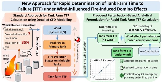
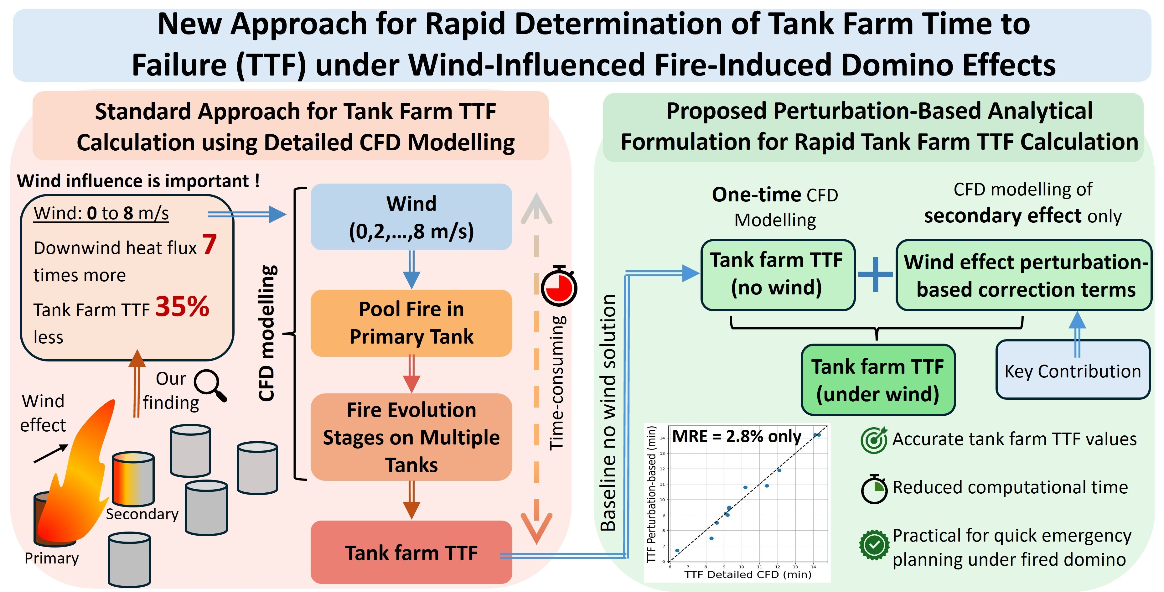
Fire-induced domino effects in tank farms can be catastrophic, particularly under wind conditions. However, due to multiple evolutionary stages, Computational Fluid Dynamics (CFD)-based modelling of wind-influenced, fire-induced domino effects and tank farm Time to Failure (TTF) calculation remain computationally expensive. This study addresses this gap by using Fire Dynamics Simulator (FDS) to model fire-induced domino effects in a tank farm and perform detailed tank farm TTF calculations across multiple wind speeds and primary pool fire scenarios. The FDS results showed that increasing wind speed from 0 to 8 m/s altered domino escalation, increasing incident heat flux on the downwind in-line tank by more than sevenfold (a 35% reduction in tank farm TTF). A new perturbation-based analytical formulation was then proposed for rapid determination of tank farm TTF under wind effects, without requiring complete CFD simulations of pool fire escalation. The formulation updates tank farm TTF under the no-wind baseline solution with wind-influenced perturbative correction terms. The proposed formulation agreed with the detailed CFD modelling-based calculation, with a mean relative error of 2.8% across all primary fire scenarios and wind conditions. This formulation provides a practical basis for rapid assessment of domino effects due to pool fire under wind conditions. However, it is calibrated for one specific six-tank configuration and crosswind directions and is not yet general.

Graphical Abstract

1. Introduction

Pool fires in tank farms have been known to promote severe fire-induced domino effects [1]. Not long ago, industrial oil depots in the United States and China were involved in multiple pool fire incidents that destroyed tank farms and caused significant human and economic losses [2,3]. The dominant heat transfer mode in open industrial pool fires is thermal radiation, which affects surrounding tanks and promotes tank failures and fire escalation [4]. The Time to Failure (TTF) of tanks is, therefore, a key factor in characterising the temporal dynamics of accident escalation and is also critical in determining the failure probability of target tanks [5,6,7].
Several correlations have been proposed to determine the TTF of atmospheric storage tanks. However, in the evolution of domino effects, some correlations apply only to a single stage, predicting the TTF of a secondary target tank exposed to a primary fire. In this regard, the TTF correlation developed by Landucci et al. [8] through extensive computer simulations under diverse fire conditions is among the most widely used. In their modelling, TTF was defined as the time at which the tank wall stresses reached the maximum allowable stress. The correlation was developed based on incident heat flux and tank volume. Similar recent studies have proposed single-stage TTF correlations for large-volume tanks [9,10]. In later stages of the domino effect, synergistic effects from multiple pool fires become relevant. In fact, modelling and analysing the synergistic effects of incident heat flux is very important to understand fire-induced domino effects in tank farms [11]. Recent studies have attempted to simulate the TTF of atmospheric tanks under the synergistic effects of incident heat flux [5]. Studies have also proposed TTF correlations for multi-stage domino effect analysis. For example, Yang et al. [12] obtained the TTF of a target tank by summing the time under the primary fire (stage 1) and the time under the synergistic effect of a secondary fire (stage 2), with the correlation coefficients fitted through numerical simulations. However, these correlations are suitable for two-stage domino evolution involving relatively smaller tank volumes. Chen et al. [13], on the other hand, proposed a correlation suitable for multi-stage domino effect modelling (stage 2 and subsequent stages). The correlation uses the incident heat flux from both the previous and current domino stages to obtain a residual time. This residual time is then added to the TTF of the previously failed tank to obtain the TTF of the target tank. These multi-stage domino effect analysis studies build upon the classical single-stage TTF correlation of Landucci et al. [8] and extend domino effect evolution analysis by accounting for the synergistic effects of multiple fires, with the TTF of the final tank corresponding to the overall tank farm TTF. The present study follows this hierarchical framework for wind-influenced, fire-induced domino evolution analyses by adopting the single-stage TTF correlation of Landucci et al. [8] together with the multi-stage TTF correlation proposed by Chen et al. [13].
It is important to note that in most previous studies on fire-induced domino effect analysis, the incident heat flux required for TTF estimation was obtained using semi-empirical models, as detailed in the cited references [14,15,16]. For instance, Khakzad et al. [17] integrated semi-empirical pool fire models with Bayesian Network (BN) to analyse domino effect propagation, and Li et al. [18] extended the domino effect risk assessment (including accident chain and multifactor contribution) due to pool fire using dynamic BN. Dueñas Santana et al. [19] used BN and fuzzy logic in determining the TTF and failure probability of tanks, while using semi-empirical-based correlation for incident heat flux estimation. Kamil et al. [20] employed Petri Nets together with semi-empirical heat flux calculations for tank farm domino analysis. Similarly, Zhou and Reniers [21] used matrix-based propagation analysis in which the incident heat flux values were obtained from semi-empirical models to represent the interaction strength between tanks. Other studies, including Chen et al. [13] and Huang et al. [22], also relied on semi-empirical models to estimate incident heat flux for fire escalation analyses. Ding et al. [23] proposed a method to model the time-dependent synergistic interaction of incident heat flux in domino effect propagation, in which the required incident heat flux was calculated using an analytical equation. Ding et al. [24] obtained the escalation index for the fire-inducing ability of the primary fire regarding a secondary tank, using incident heat flux obtained from a semi-empirical model.
Although these studies contributed significantly to understanding the evolution of the domino effect, the wind effect was not their particular emphasis. This is primarily because conventional semi-empirical pool fire models possess inherent limitations in representing realistic flame behaviour under wind effects. In particular, these models generally approximate the flame as a cylindrical geometry under both no-wind and wind conditions [25], making them less suitable for accurately predicting the effects of flame tilt under complex wind scenarios [26,27]. Moreover, these semi-empirical models were originally developed for estimating incident heat flux from a single primary fire to a secondary target [16], limiting their suitability in complex domino evolution involving multiple simultaneous fires and dynamic propagation pathways.
Accurate representation of wind effects is essential, as they play a crucial role in overall fire escalation behaviour [28,29]. Consequently, a few recent studies have adopted Computational Fluid Dynamics (CFD) to model the wind-influenced, fire-induced domino effect. Unlike semi-empirical pool fire models, CFD can capture detailed flame dynamics, flame tilt behaviour, and transient heat transfer under both no-wind and wind conditions [30]. For example, Jujuly et al. [31] simulated liquefied natural gas pool fires using CFD and demonstrated that wind strongly influences the potential for fire escalation to adjacent tanks. Similarly, Ahmadi et al. [27] investigated dike pool fires under wind conditions and showed that wind can substantially alter the behaviour of fire-induced domino propagation. Yang et al. [32] and Li et al. [33] further extended CFD application to investigate multiple simultaneous pool fires and their influence on fire-induced domino escalation to secondary tanks under wind effects. Among the available CFD tools for fire modelling, Fire Dynamics Simulator (FDS) is considered one of the most suitable software tools because it is specifically designed for fire-driven simulations (including wind effects) and has been extensively validated [34]. Nevertheless, despite the improved accuracy of CFD, its application to the complete evolution of the fire-induced domino effect in tank farms and subsequent TTF calculation remains relatively limited [35,36]. One of the primary reasons for this is the high computational cost of transient fire CFD simulations involving multiple tanks and varying wind conditions [9]. This may affect their practicality in rapid risk assessment. In this regard, recent studies have attempted to use Machine Learning (ML) to rapidly predict tank TTF due to pool fire [37,38]. However, in calculating TTF, these approaches do not utilise CFD modelling to obtain the heat flux distribution, which provides a more accurate representation of pool fire dynamics under complex conditions, including wind. There remains a need for an approach that retains the physical representation provided by CFD while reducing the computational burden of repeated full-scale simulations of fire-induced domino evolution under different wind conditions.
Therefore, to address this concern, this study uses FDS and first performs detailed CFD modelling of the evolution of the fire-induced domino effect due to a pool fire in a complete tank farm, thereby obtaining tank farm TTFs under varying wind speeds. Then, an alternative approach is proposed for quick determination of tank farm TTF under wind conditions, which efficiently uses CFD simulations to obtain the incident heat flux required for TTF calculations. In this proposed approach, the tank farm TTF under wind conditions is determined using a perturbation-based analytical formulation that updates the no-wind baseline TTF using wind-induced perturbative correction terms. Here, the TTF of the tank farm under no-wind conditions can be obtained from a one-time CFD simulation. In the perturbative correction terms, only the TTF of the secondary tanks under both no-wind and wind conditions is required to be obtained from CFD modelling. Hence, using this perturbation-based analytical formulation, the TTF for the entire tank farm under wind conditions is determined, without requiring detailed CFD simulations of the full domino effect. Perturbation-based modelling and related techniques, including reduced-order and surrogate modelling, have been widely used in engineering and applied mechanics to obtain approximate analytical solutions for complex nonlinear systems [39,40]. These include wave propagation in nonlinear media [41,42], feature selection in high-dimensional datasets [43], and the iterative improvement of ML forecasts [44]. In the context of fire risk assessment, reduced-order and surrogate modelling approaches have been integrated with ML techniques for wildfire progression prediction [45,46] and applied to smoke transport modelling and heat and mass transfer analysis in high-rise buildings, where detailed CFD simulations are computationally demanding [47]. To the authors’ knowledge, perturbation-based modelling has not previously been applied to represent wind-induced deviations from a baseline no-wind solution to rapidly predict tank farm TTF due to pool fires, while preserving the physical interpretation of CFD simulations. As mentioned earlier, addressing this gap is important for fire-induced domino effect analysis under wind conditions, where evaluating multiple escalation scenarios remains challenging due to the computational cost of detailed transient CFD simulations [9]. Therefore, this study extends CFD-based fire-induced domino effect modelling by developing a perturbation-based analytical formulation to rapidly estimate tank farm TTF under wind conditions. The proposed framework translates detailed CFD-derived domino evolution behaviour into a simplified analytical formulation, retaining the predictive capability of CFD while improving computational efficiency and practical applicability for risk assessment and emergency planning.

2. FDS Governing Equations

In this study, FDS was employed, which is specifically designed for fire-driven flows. It numerically solves the low-Mach-number form of the Navier–Stokes equations, which retains buoyancy- and heat-driven flow characteristics typical of the fire environment [48]. Since the objective of this study is to evaluate wind-induced thermal exposure and domino escalation between tanks, particular emphasis is placed on selecting and presenting the governing equations most relevant to accurately capturing wind-modified flame dynamics and predicting incident heat flux. The respective governing equations and associated modelling choices adopted for this purpose are presented below.

2.1. Conservation of Momentum

The conservation of momentum equation is expressed as Equation (1) [49]:
( ρ u ) t + . ( ρ u u ) = p + . τ i j + ρ f
where ‘ ρ ’ is the fluid density, ‘ u ’ is the velocity vector of the fluid flow, ‘ t ’ is the time, ‘ ’ is the gradient operation, ‘ p ’ is the pressure, ‘ τ i j ’ is the viscous stress tensor, and ‘ f ’ represents body forces (e.g., gravity). In pool fire simulations, the momentum equation is important for predicting flame plume and smoke behaviour, buoyancy-driven turbulence, and entrainment of surrounding air.

2.2. Conservation of Mass

The conservation of mass equation is expressed as Equation (2) [49]:
l n ρ t + u . l n ρ + . u = 0
where the term . u is the divergence of the velocity field. In pool fire modelling, it is necessary to capture density variations caused by heating, expansion of combustion gases, and air entrainment into the flame region.

2.3. Conservation of Energy

Energy conservation is expressed as the sensible enthalpy transport formulation, as shown in Equation (3) [49]:
ρ h s t = Q ˙ + . ( k T ) . α h s , α J α . q ˙ r
where ‘ h s ’ is sensible enthalpy, ‘ Q ˙ ’ is the heat release rate, ‘ k ’ is thermal conductivity, ‘ T ’ is temperature, ‘ α ’ is species, ‘ J α ’ is the species diffusion flux vector, and ‘ q ˙ r ’ is the radiative heat flux vector. Since the present study focuses on tank farm fire modelling, only the dominant energy transport mechanisms relevant to fire development are considered, including chemical heat release from combustion, thermal conduction, species enthalpy transport, and radiative heat transfer.

2.4. Combustion Modelling

Combustion in FDS is modelled using a single-step mixture fraction-based combustion model for fuel–air mixtures, expressed as Equation (4) [50].
Z = s Y F ( Y O Y O ) s Y F I Y O
where ‘ Z ’ is the mixture fraction, ‘ Y F ’ is the fuel mass fraction, ‘ Y O ’ is the oxygen mass fraction, ‘ Y O ’ is the ambient oxygen mass fraction, ‘ Y F I ’ is the fuel mass fraction in the fuel stream, and ‘ s ’ is the stoichiometric coefficient. Z describes the local state of fuel–air mixing, where Z = 1 represents a pure fuel stream and Z = 0 represents ambient air conditions. The model assumes that combustion is mixing-controlled, with fuel and oxygen reactions occurring rapidly relative to the mixing process [51].

2.5. Radiation Transport Modelling

Thermal radiation modelling under sooty fire conditions is conducted by solving the radiation transport equation (RTE) for a grey gas, expressed as Equation (5) [52].
d I d x = k a ( I b I )
where ‘ I ’ is the radiative intensity, ‘ I b ’ is the blackbody intensity, ‘ x ’ is the optical path of radiation propagation, and k a is the grey gas absorption coefficient. The grey gas model is the default radiation model in FDS. It has a low computational cost and has been shown to provide accurate radiative transport predictions for hydrocarbon fire simulations [52]. This model has also been widely adopted for near- and far-field radiative transport in pool fire simulations in tank farms using FDS [27,28,36]. According to the FDS User Guide, more detailed radiation models are generally computationally expensive and are recommended for non-sooting fuels [48].

2.6. Wind Modelling

Wind is prescribed using the atmospheric power-law profile (PROFILE = ‘ATMOSPHERIC’), which is suitable for fire simulation in an open environment [51]. It accounts for the variation in wind velocity with height above the ground surface, as expressed in Equation (6) [48].
u ( z ) = u o ( z z o ) r
where ‘ u ( z ) ’ is the wind velocity at the elevation ‘ z ’, ‘ u o ’ is the velocity at the reference height “ z o ”, and ‘ r ’ is the power-law exponent. The reference height is taken as 10 m, following the convention used in meteorological wind measurements and atmospheric wind profile modelling in FDS [53,54]. The power-law exponent is set to 0.143, as used in atmospheric wind profile applications in FDS [53]. This value corresponds to open, flat terrain with low surface roughness, which is consistent with the atmospheric conditions considered in the present tank farm simulations.

3. Methodology

This section presents methodological details, including FDS model validation (with and without wind), the case study description, the mesh independence study, the methodologies for calculating tank farm TTF using detailed CFD-based modelling, and the proposed perturbation-based analytical formulation.

3.1. FDS Modelling Validation Against Experiment

A pool fire model was developed in FDS Version 6.5.3 to validate the modelling approach against an experiment conducted by Yamaguchi and Wakasa [55]. The incident heat flux was measured at a height of 0.45 metres (m) above the ground and at positions of L/D = 2 and 3 from the centre of a 30 m diameter kerosene pool fire. ‘L’ is the horizontal distance (m) of the heat flux device from the pool fire centre, and ‘D’ is the diameter of the pool fire. The height of the heat flux measurement corresponds to the tank height specified in the experimental configuration by [55], and has also been adopted by other studies performing FDS validation against the same experiment [27]. Since the experiment by Yamaguchi and Wakasa [55] did not report incident heat flux measurements under wind conditions, a propane pool fire experiment conducted by Miao et al. [56] was selected, as it was specifically performed to investigate incident heat flux under wind effects. From Miao et al.’s [56] experiment, a 0.3 m diameter propane pool fire (33 kW heat release rate) was considered, with heat flux measurements obtained using gauges placed at the base level and at radial distances from the pool fire centre. The wind speed for validation was 2.5 m/s (crosswind). The validation considered four heat flux measurement locations, with the first gauge positioned 0.21 m from the pool fire centre and the remaining three gauges spaced at 0.06 m intervals. The measurement locations enabled validation of the incident heat flux at both near and distant locations from the fire source. The purpose of these validation cases was to assess the capability of FDS to reproduce the dominant physical mechanisms governing fire-induced thermal radiation and incident heat flux under both no-wind and wind-influenced conditions. For consistency, we ensured that the fuels used in the validation cases and the case study simulations (discussed later) were hydrocarbon pool fires. Both experiments were carried out without a fire suppression system. All the details of the parameters used for modelling these experiments in FDS are provided in Table 1.
As shown in Table 1, several parameters are important to define for accurate modelling of pool fires in FDS. Among them, a few are highly important. For example, soot yield and radiative fraction directly influence the thermal radiation field and the incident heat flux to the targets. Experimental studies show that increasing the radiative fraction and soot yield increases the incident radiative heat flux [57]. Hence, care should be taken to ensure that the appropriate values from the standards are used for these two parameters. It is important to note that, for the Miao et al. [56] experiment, setting the soot yield to zero was a modelling decision adopted in the FDS simulation based on the complete combustion assumption reported in the original study. This choice is supported by previous studies reporting low soot production from propane fires, with soot yield decreasing with increasing wind velocity [58], and by an experimental study reporting a zero soot yield for a propane pool fire [59]. Another key parameter in defining a pool fire is the mass loss rate per unit area (MLRPUA). This governs the heat release rate and, consequently, influences the intensity of thermal radiation. The value of MLRPUA varies with fuel and burning conditions; therefore, it should be carefully determined. The number of solid angles is also an important parameter for thermal radiation modelling in FDS. An insufficient number of solid angles used for discretisation can result in a non-uniform radiation distribution [34]. This effect becomes particularly significant when the target surfaces are located far from a localised radiation source [60]. A prior study determined 500 solid angles as sufficient [27], and, thus, this value was used in the validation and case study modelling.
For all the simulations, Large Eddy Simulation (LES) was adopted as the turbulence modelling approach, as it is the standard method for fire dynamics simulations. The default Deardorff subgrid-scale (SGS) turbulence model implemented in FDS Version 6.5.3 was employed. The Deardorff SGS model is recommended by FDS for fire dynamics simulations [61]. Previous studies have reported that alternative SGS turbulence models produce similar incident radiative heat flux predictions for pool fires, indicating negligible sensitivity of radiation predictions to the choice of SGS model [27]. The combustion process was represented using simple chemistry, a single-step reaction, and a mixing-controlled combustion model. To replicate an open environment, all domain boundaries were assigned as ‘OPEN’ boundaries, except the wind inlet boundary, where the prescribed atmospheric wind profile was applied. The ground surface was specified as an ‘INERT’ boundary. When using LES, the selection of an appropriate numerical grid is essential, as insufficient spatial resolution may reduce the accuracy of the predicted flow field and associated fire characteristics [62]. In this regard, the validation simulations were conducted using a relatively finer mesh to ensure adequate resolution, consistent with previous FDS-based studies [56]. The total numbers of mesh cells used for the Yamaguchi and Wakasa [55] and Miao et al. [56] experiments were 9 million (grid size 0.75 m) and 5.8 million (grid size 0.01 m), respectively. In FDS modelling, the mesh resolution is usually characterised by D / d x , with larger values corresponding to a better resolution (a greater number of cells and smaller grid size). ‘ d x ’ is the grid size in m and ‘ D ’ is the characteristic fire diameter, which, in accordance with the FDS guidelines, is defined as Equation (7) [48]:
D =   ( Q ˙ ρ a C p T a g ) 2 5
Here, ‘ Q ˙ ’ is the total heat release rate (kW) of the fire; ‘ ρ a ’, ‘ C p ’, and ‘ T a ’ are the density (kg/m3), specific heat (J/kgK), and temperature (K) of the ambient air, respectively. ‘ g ’ is the gravitational acceleration (m/s2).
The mesh resolutions for both these experiments correspond to D / d x values of approximately 22 and 24 for the Yamaguchi and Wakasa [55] and Miao et al. [56] experiments, respectively. Using a fine mesh directly is feasible for single validation cases; however, for full-scale CFD simulations involving multiple scenarios, an additional mesh-independence study is needed to identify a mesh size that provides sufficient accuracy while remaining computationally feasible. Therefore, a mesh independence study was performed only for the case-study simulations, and the results are presented in the subsequent section.
Table 1. Fire Dynamics Simulator (FDS) input parameters used for pool fire modelling and validation.
Input ParametersExperiment (No Wind)Experiment (with Wind)
StudyYamaguchi and Wakasa [55]Miao et al. [56]
FuelKerosenePropane
Pool size (m)30 [55]0.3 [56]
Heat of combustion (kJ/kg)43,200 [63]43,700 [64]
Soot yield (kg/kg)0.042 [63]0.0 [56]
Radiative fraction (-)0.08 [63]0.3 [56]
MLRPUA (kg/m2s)0.039 [16]0.008 [56]
Number of solid angles (-)500 [27]500 [27]
Wind speed (m/s)-2.5 [56]
Ambient temperature (°C)21 [27]30 [56]
Model domain size (X × Y × Z) (m)200 × 200 × 1001.5 × 3 × 1.3
Figure 1 shows the validation results of the FDS modelling against the experimental studies. Figure 1a corresponds to the no-wind condition, whereas Figure 1b represents wind conditions of 2.5 m/s. As shown in Figure 1a, the FDS modelling results are in agreement with the experimental results reported by Yamaguchi and Wakasa [55], with a maximum deviation of approximately 7% in the predicted incident heat flux. Similarly, under the wind condition, the FDS modelling predictions shown in Figure 1b also agree reasonably well with the experimental data reported by Miao et al. [56], with the predicted incident heat flux values differing by 4–10% across the four measurement devices. In general, this difference is considered acceptable in fire modelling research [65,66].

3.2. Case Study

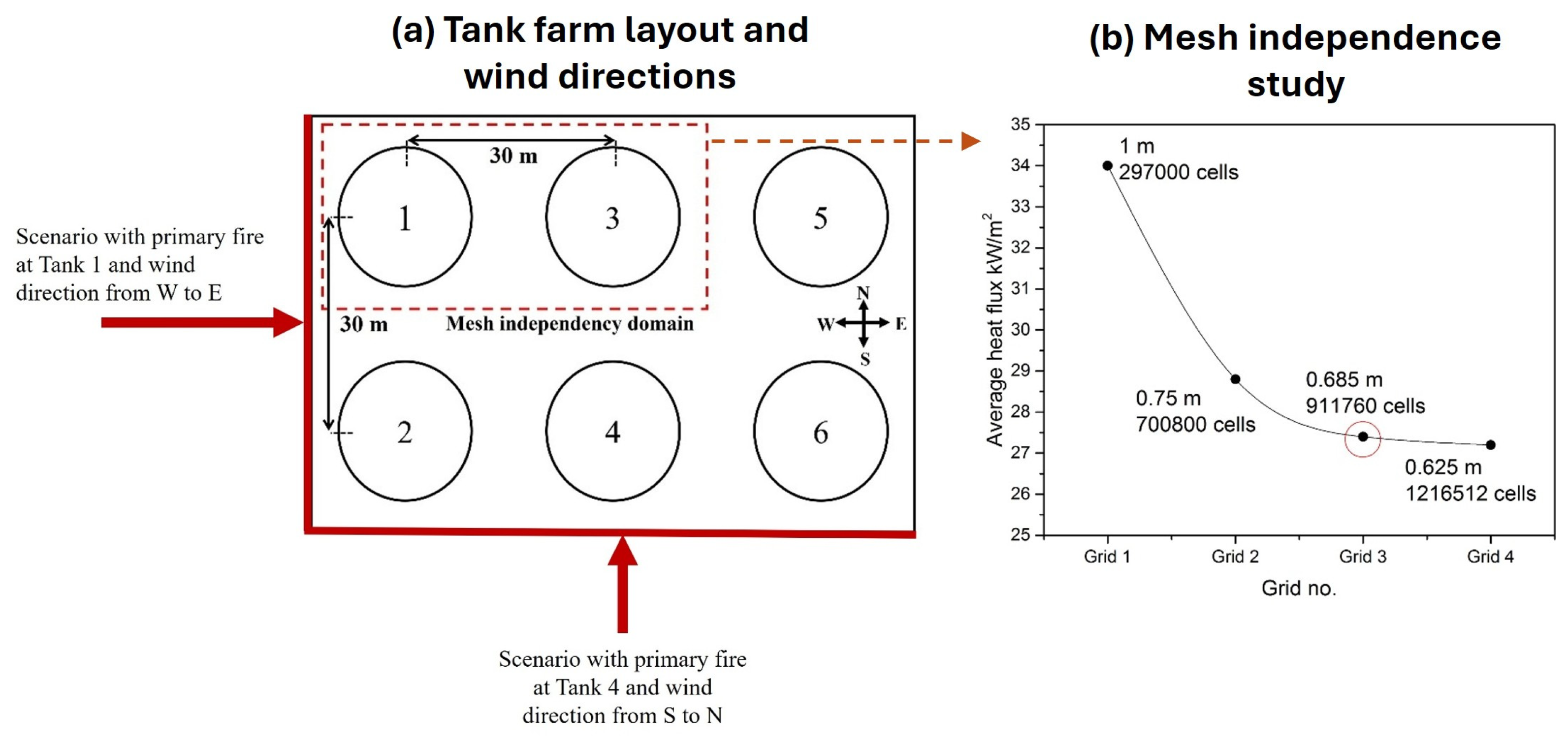
The proposed methodology was developed based on a case study from Zhou et al. [67]. As shown in Figure 2a, the oil storage depot case study comprises 6 non-spherical atmospheric gasoline storage tanks. The tanks are equal in size, with a diameter of 20 m and a height of 10 m. The separation distance between the tanks is 30 m, and the credible accident scenario for all tanks is a pool fire [17]. The distances between the tanks are within the acceptable distance set by the National Fire Protection Association (NFPA) 30 [68]. The case study considers no fire suppression system, establishing a worst-case condition. Two primary accident scenarios, (a) primary fire at Tank 1 and (b) primary fire at Tank 4, are used for the domino escalation analysis. When the primary fire is at Tank 1, the wind direction is from west (W) to east (E), whereas for the primary fire at Tank 4, the wind is directed from south (S) to north (N), as shown in Figure 2a. While also accounting for the no-wind condition, the atmospheric wind speeds considered in this study are 1, 2, 4, 6, and 8 m/s, which provide extensive coverage and fall within the range of frequently occurring wind speeds in Malaysia [69]. The FDS input parameters required to model pool fires in a tank farm are given in Table 2.
The results of the mesh independence study performed for the tank farm case study are depicted in Figure 2b. The mesh independence study considered four grid resolutions corresponding to D / d x of approximately 15, 20, 22, and 23, respectively, following the mesh resolution methodology recommended in the FDS User Guide [48]. The number of cells and their corresponding grid sizes at the given grid resolution are shown in Figure 2b. To further confirm mesh adequacy, the optimal grid size was selected based on the results of the mesh independence study. To save simulation time, the primary fire at Tank 1 and an adjacent Tank 3 (shown in Figure 2a) is included in the test domain to determine the optimal grid size for complete simulation. From Figure 2b, it is evident that reducing the grid size from 0.685 m to 0.625 m resulted in a 0.7% change in heat flux, indicating that a grid size of 0.685 m (which corresponds to D / d x of 22) is optimal for CFD simulations. As the mesh independence study was performed on a representative subdomain that captured the dominant fire-induced flow and heat transfer phenomena from the primary fire, the selected grid size was subsequently adopted for the full six-tank simulations using the same physical models and numerical settings. This approach is also adopted in the other CFD modelling literature on mesh independence studies for similarly large domains [70]. This uniform grid extension is justified because all tanks in the full domain share identical geometric configurations and spacing; hence, the sufficiently fine mesh resolution optimised for the subdomain remains valid and representative for the entire tank farm.
Table 2. FDS input parameters used to model pool fire in tank farm case study.
Input ParametersValuesReferences
FuelGasoline[67]
Pool diameter (m)20[67]
Heat of combustion (kJ/kg)44,100[71]
Soot yield (kg/kg)0.038[15]
Radiative fraction (-)0.4[15,48]
Density (kg/m3)715
MLRPUA (kg/m2s)0.069[16]
Number of solid angles (-)500[27]
Model domain size (m)120 × 90 × 55

3.3. Methodology for Tank Farm TTF Calculation Using Detailed CFD Modelling

To perform the tank farm TTF calculation using detailed CFD modelling, a single tank in the farm is treated as the primary unit initiating the fire-induced domino effect. In the present study, Tanks 1 and 4 are treated as primary tanks for pool fires. When the primary tank fails and gives rise to a pool fire, the incident heat flux on the surrounding tanks is measured using “radiative heat flux gas” devices in FDS. The incident heat flux from the primary pool fire is averaged when it becomes quasi-steady and is used to calculate the TTF of nearby secondary tanks using Equation (8) [8,72]. Equation (8) was developed based on comprehensive simulations and validations covering various fire exposure conditions, including heat loads on tanks from distant-source fires and direct flame engulfment/impingement [8]. The latter represents a fire exposure condition that may also occur under wind-influenced, tilted flames. This correlation has also been utilised in several recent studies to estimate the TTF of secondary tanks due to primary fires and in investigations considering wind effects [7,12,19,33,73]. However, it should be noted that the correlation given in Equation (8) was developed for atmospheric storage tanks with a design pressure of 0.1 megapascals and tank volumes ranging from 25 to 17,500 m3. Therefore, verifying compatibility with these boundary conditions is necessary before application. In the present study, Equation (8) is considered applicable because the tanks investigated in the case study represent atmospheric storage tanks and their volumes fall within the design range.
    T T F i = { ( e x p [ 1.128 l n ( I i ) 2.667 × 10 5 V i + 9.877 ] 60 ) }                 i = 1 , 2 , 3 , , n
where ‘ i ’ is the number of tanks exposed to a primary pool fire; ‘ T T F i ’ is the failure time of exposed tanks expressed in minutes (mins); ‘ I i ’ is the incident heat flux (kW/m2) of exposed tanks; and ‘ V i ’ is the tank volume (m3).
The tank with the earliest failure time among all tanks is designated as the secondary unit and modelled as a pool fire. The secondary burning pool fire synergistically contributes to the remaining unburned tanks in the form of simultaneous pool fires, and the superimposed incident heat flux on tanks that are yet to fail is also measured by “radiative heat flux gas” devices in FDS. As mentioned in the introduction, Equation (8) is applicable only for calculating the TTFs of tanks under primary pool fires. The domino effect develops in stages, with each stage occurring as a tank additionally gives rise to a pool fire. Therefore, the accumulated TTFs of non-spherical tanks due to the synergistic effect of multiple pool fires in progressive domino effect evolution stages are obtained using Equations (9) and (10), which are adopted from [13].
      t i , r e s , S = ( I i , S I i , S 1 ) 1.13 ( t i , S 1 t m i n i m u m   f a i l u r e , S 1 ) i = 1 , 2 , 3 , , n  
T T F i , a c c u m u l a t e d , S = t i , r e s , S + t m i n i m u m   f a i l u r e ,   S 1
t i , r e s , S ’ is the residual time (mins) of tank ‘ i ’ in the current stage ‘ S ’; ‘ I i , S ’ and ‘ I i , S 1 ’ are the incident heat fluxes in (kW/m2) received by tank ‘ i ’ in the current stage ‘ S ’ and at the previous stage ‘ S 1 ’, respectively; ‘ t i , S 1 ’ is the elapsed time (in mins) of tank ‘ i ’ in the previous stage ‘ S 1 ’; ‘ t m i n i m u m   f a i l u r e , S 1 ’ is the minimum time to fail of a failed tank (mins) in stage ‘ S 1 ’; and ‘ T T F i , a c c u m u l a t e d , S ’ is the accumulated TTF of tank ‘ i ’ in stage ‘ S ’ due to synergistic effects, expressed in mins.
Equation (9) is a recurrence formula that updates the residual time of a tank based on the incident heat fluxes from the previous and current stages of domino evolution; the ratio of these incident heat fluxes serves as an adjustment factor. Residual time represents the acceleration of domino effect evolution due to the superimposition and synergistic effects of pool fires [13]. The exponent (−1.13) in this expression for atmospheric tanks is the empirical regression coefficient originally obtained by Landucci et al. [8] and also used in the formulation by Chen et al. [13]. This negative exponent reflects an inverse relationship between incident heat flux and TTF. Equations (9) and (10) were originally developed and validated by Chen et al. [13] specifically for fire-induced domino effect evolution under wind conditions, confirming their applicability to the wind-influenced scenarios considered in the present study. Using Equations (9) and (10), the accumulated TTF for each tank is sequentially determined at each stage of domino evolution. As the domino effect progresses, adjacent tanks continue to fail, subsequently giving rise to pool fires, modelled as synergetic pool fires in FDS, until all tanks within the tank farm have failed. The accumulated TTF for the final failed tank represents the overall TTF of the tank farm. This is referred to as the “Tank Farm TTF using Detailed CFD Modelling” in the results section. This process is repeated with various wind speeds and primary fire conditions, as mentioned in the case study section.

3.4. Tank Farm TTF Calculation Using Proposed Perturbation-Based Analytical Formulation

Although the “Tank Farm TTF using detailed CFD Modelling” calculation provides a comprehensive representation of domino effect escalation and tank farm TTF estimation, it is computationally expensive, particularly when multiple wind speeds and primary fire scenarios are considered. A balance can be achieved by streamlining the physical approximations in the models [74]. One such known mathematical approach involves perturbation techniques to obtain approximate solutions for highly complex problems that are otherwise computationally expensive to solve [75,76]. In this approach, perturbations (correction terms) are added to the known initial (baseline) solution [77], allowing the calculation of precise mathematical corrections that update the initial solution toward an accurate approximation of the solution of a targeted complex problem. As explained in the introduction, this and similar approaches have been used in various engineering domains, including fire risk assessment contexts.
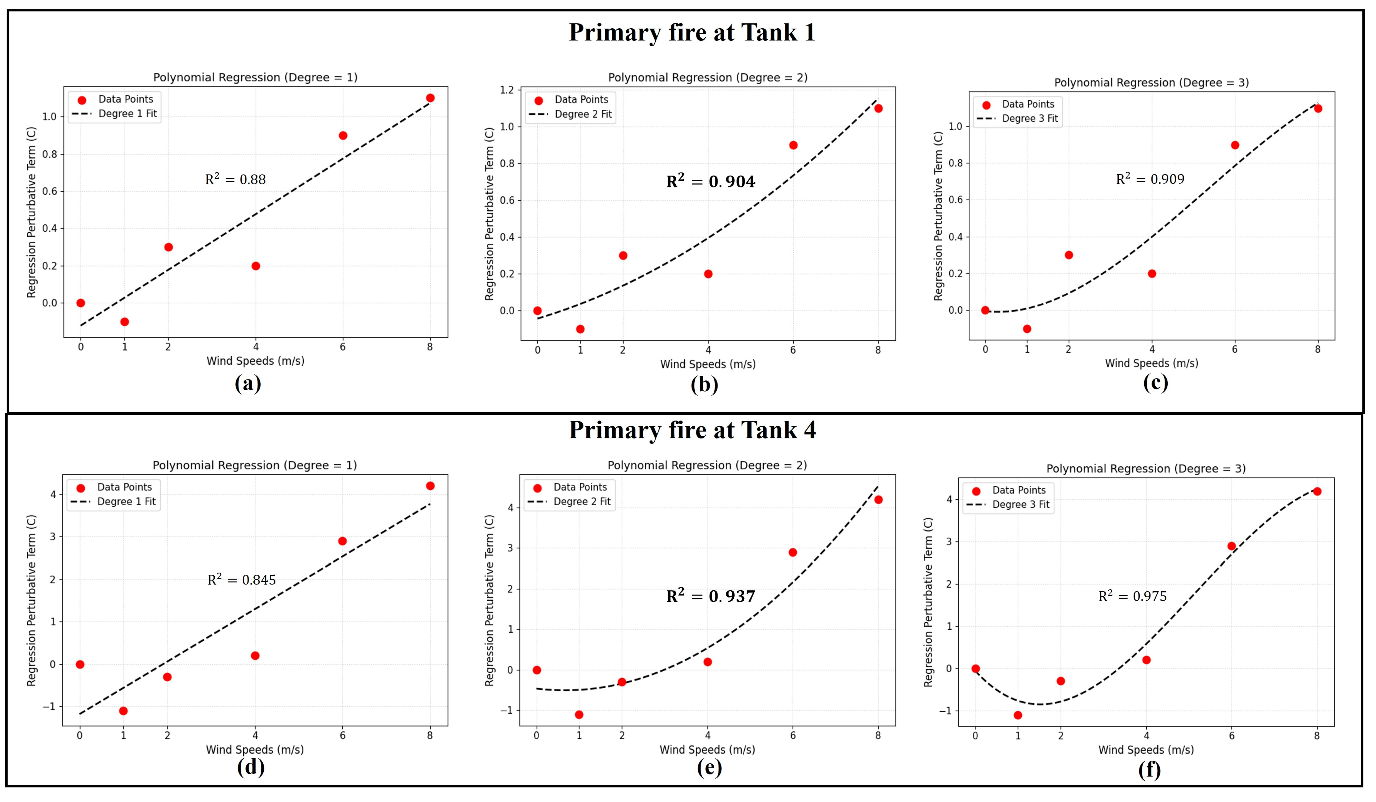
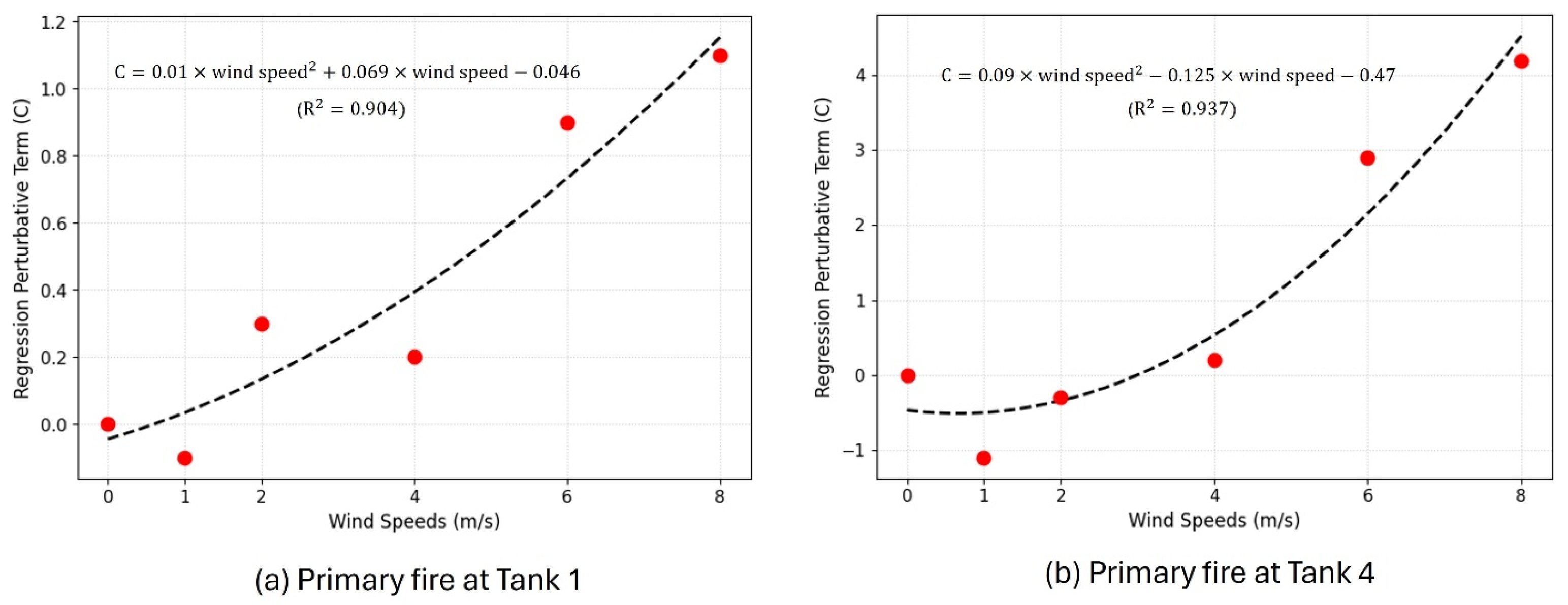
In this study, a perturbation-based analytical approach is proposed to determine the TTF of tank farms exposed to pool fires under wind conditions, providing an innovative framework for analysing fire-induced domino effects. In this analytical calculation, the no-wind tank farm TTF serves as the initial or baseline solution, while the difference between the secondary tank TTF under wind and no-wind conditions is treated as the first-order perturbative correction term. The secondary tank is selected for this first-order term because it directly experiences the wind-modified incident heat flux, serving as a key indicator of the initial wind effects on fire-induced domino escalation dynamics. An additional regression perturbative term ( C ) is integrated into the analytical approximation to account for higher-order perturbative variations, specifically the difference between the tank farm TTF from detailed calculation and the analytical calculation with the first-order perturbative correction term. The regression perturbative term varies with the primary fire scenarios and is expressed as a function of wind speed, valid for 0–8 m/s. The regression plot, R2 values and corresponding equations are presented in Figure 3. As shown in Figure 3, the regression plots are quadratic, providing a good fit to the data for both primary fire scenarios. A sensitivity check of different functional forms is performed, with the results presented in Figure A1 in Appendix A. Although the cubic form yields slightly higher R 2 values, the improvement is negligible in the scenario (primary fire at Tank 1), whereas the cubic fit for the scenario (primary fire at Tank 4) exhibits non-monotonic, oscillatory behaviour between data points, indicating overfitting. The quadratic form is, therefore, adopted, as it captures the observed nonlinear trend while avoiding overfitting, given the set of wind-speed conditions used in the regression. The explicit quadratic regression equations are provided in Appendix A (Equations (A1) and (A2)) for reproducibility.
It is also important to highlight that the term ‘perturbation-based’ used throughout this paper refers to the structural form of the approach—a baseline (no-wind) solution combined with ordered perturbative correction terms [77]. The correction terms are not infinitesimal perturbations; however, their sequential structure follows the concept of a perturbation-based correction approach. As explained above, the first-order term captures the dominant wind-induced deviation, and the second-order regression perturbative term ( C ) captures the residual higher-order variation. The perturbative correction terms remain smaller than the baseline solution, while the second-order term is, in turn, smaller than the first-order term. This general decreasing structure across correction orders is consistent with a perturbation-based framework [78]. Ultimately, this perturbation-based analytical formulation computes the total tank farm TTF under wind conditions by summing the baseline solution with the corresponding perturbative terms. The complete perturbation-based analytical formulation, along with its effectiveness in determining the tank farm TTFs, is presented in the results section.

4. Results and Discussion

This section covers the results of the study. These include the spatial contours of incident heat flux as the wind-influenced domino effect evolves, initiated by different primary fire scenarios. This section also presents the results and discussion of TTF for individual tanks under varying wind conditions, highlighting the implications for emergency response operations. This section also shows the results of tank farm TTF calculations using detailed CFD modelling and the proposed perturbation-based analytical formulation.

4.1. Incident Heat Flux Contours in Wind-Influenced Domino Evolution

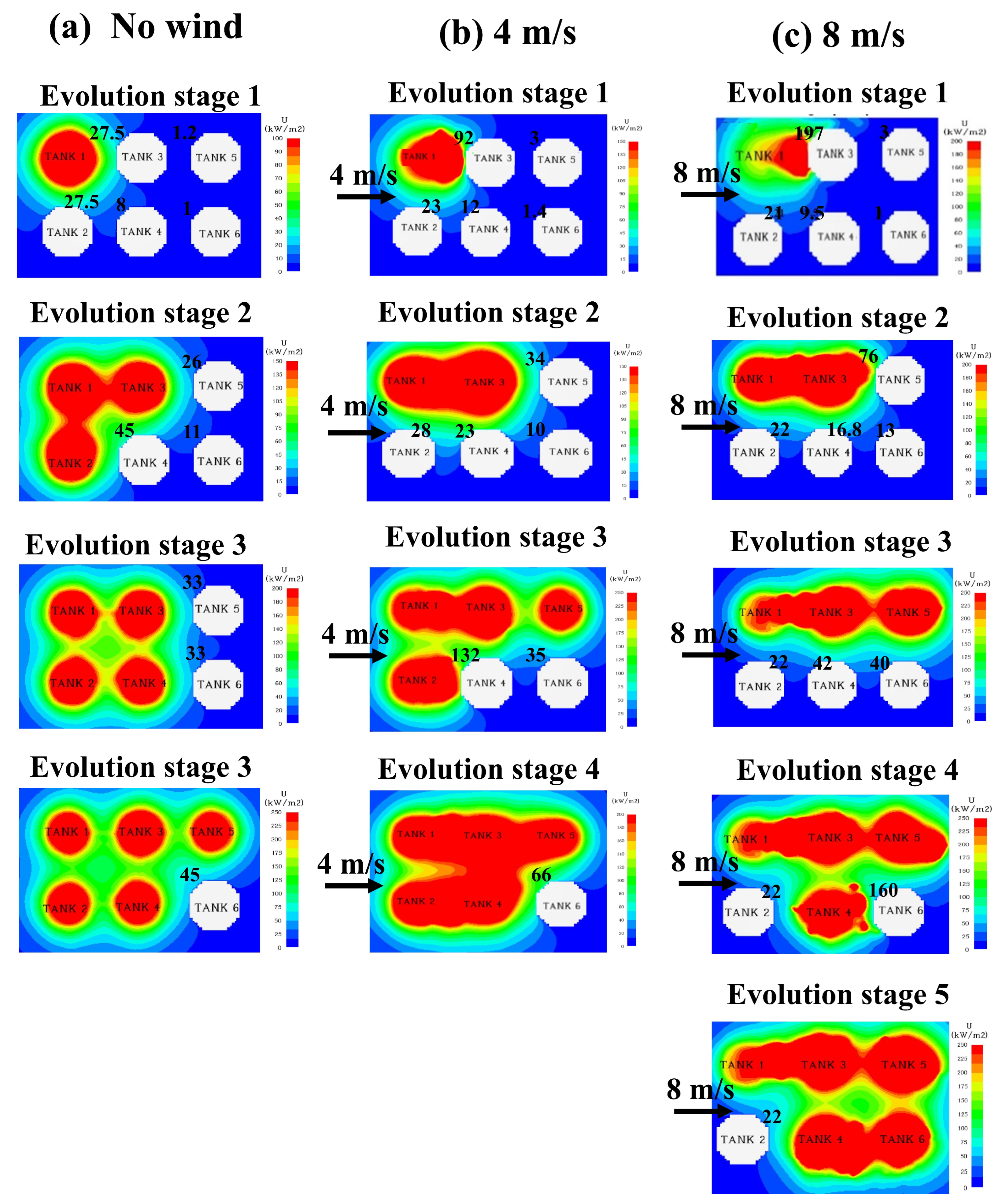
Figure 4 shows the spatial distribution of incident heat fluxes obtained from FDS during the complete domino evolution process within the tank farm under varying wind conditions, beginning with the primary fire at Tank 1. The contours depict incident heat fluxes during domino evolution at selected wind speeds. However, the full range of wind speeds defined in the case study is accounted for in the calculations. Following the failure of the primary tank, subsequent tanks progressively fail according to their TTFs and are converted into equivalent pool fire sources, enabling sequential fire escalation (domino effect) to be simulated until complete tank farm failure occurs.
Under no-wind conditions (Figure 4a), the incident heat flux distribution remained relatively symmetric around the burning tanks, resulting in more balanced incident heat fluxes among neighbouring tanks. However, as wind speed increased, the thermal radiation field became more directional, substantially amplifying the incident heat flux on downwind in-line tanks while reducing thermal exposure on offset tanks. As shown in Figure 4b,c, the incident heat flux at the in-line Tank 3 due to the primary fire at Tank 1 increased significantly with increasing wind speed because of increased flame tilt in the wind direction. Compared with the no-wind condition, the incident heat flux at Tank 3 increased by three and seven times at wind speeds of 4 and 8 m/s, respectively. Conversely, the incident heat flux at the offset Tank 2 gradually decreased with increasing wind speed, becoming approximately 1.3 times lower at 4 and 8 m/s, respectively, due to reduced influence of the flame tilt direction. The cumulative incident heat flux distributions for the remaining tanks across all domino evolution stages further demonstrate that wind not only modified the magnitude of incident heat fluxes but also significantly altered the sequence and directionality of domino escalation within the tank farm.
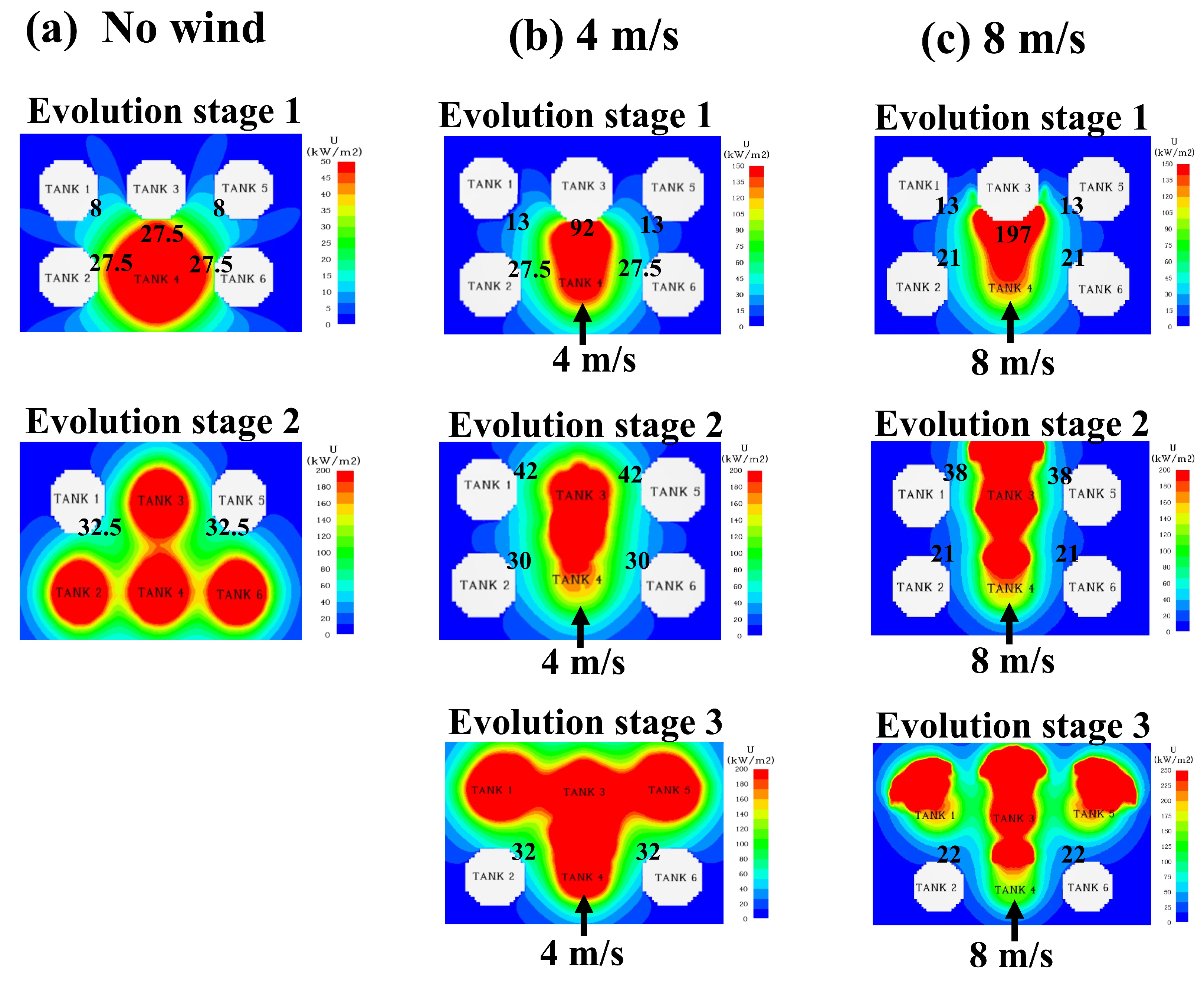
Figure 5 presents the incident heat flux distribution contours during the wind-influenced domino evolution process initiated by a primary fire at Tank 4. Compared with the corner-located primary fire scenario at Tank 1, the domino escalation behaviour for the centrally located Tank 4 exhibited substantially faster progression with fewer domino evolution stages. Under no-wind conditions (Figure 5a), the domino evolution initiated from Tank 4 terminated within only two stages, whereas the primary fire at Tank 1 had four stages for complete tank farm involvement. A similar trend was observed at wind speeds of 4 and 8 m/s, as shown in Figure 5b,c. The reduced number of domino stages is primarily due to simultaneous thermal interactions among multiple adjacent tanks and the centrally located burning tank, resulting in concurrent pool fire formation within a single domino stage. Such behaviour is particularly hazardous because the rapid escalation and simultaneous involvement of multiple tanks can significantly reduce available emergency response time and potentially lead to uncontrollable fires. As in the case of the primary fire at Tank 1, under no-wind conditions, the thermal radiation field from the pool fire at Tank 4 resulted in nearly equal incident heat fluxes on the adjacent offset Tanks 2 and 6 and the in-line Tank 3. However, at higher wind speeds, flame tilt significantly amplified the incident heat flux on the in-line, downwind tanks while reducing it on the offset tanks, following a trend similar to that observed in the primary fire scenario at Tank 1.

4.2. Tank Farm TTF Using Detailed CFD Modelling

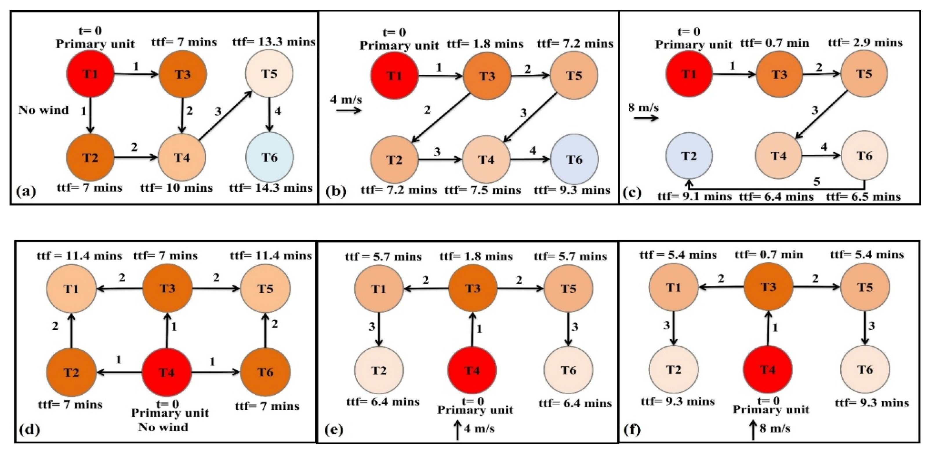
Figure 6 illustrates the domino escalation path and corresponding TTFs of tanks under varying wind conditions for the two primary fire scenarios. The overall TTF of the tank farm is determined by the accumulated failure time corresponding to the last failed tank in the domino sequence. The associated TTF calculations are obtained through the detailed calculation steps outlined in Equations (8)–(10).
As shown in Figure 6a, under no-wind conditions with the primary fire initiated at Tank 1, Tanks 2 and 3 failed simultaneously after 7 min. Subsequently, Tank 4 failed at 10 min, followed by Tank 5 at 13.3 min and finally Tank 6 at 14.3 min, representing the overall TTF of the tank farm. However, under the 4 m/s wind condition shown in Figure 6b, the TTFs of all tanks except Tank 2 decreased substantially. The TTF of Tank 3, located directly in the downwind direction of Tank 1, reduced from 7 min under no-wind conditions to only 1.8 min at 4 m/s wind speed, corresponding to an approximate 74% reduction in failure time. The wind-induced flame tilt led the domino path toward a directional sequence of Tank 1 → Tank 3 → Tanks 2 and 5 → Tank 4 → Tank 6. As seen in Figure 6b, under 4 m/s wind conditions, Tank 5 became significantly more vulnerable compared to Tank 2 despite being farther from the primary fire. This was because of its location in the in-line downwind direction. Consequently, Tanks 2 and 5 failed simultaneously at 7.2 min. Note that Tank 5 failed much later under no-wind conditions. The overall tank farm TTF decreased from 14.3 min to 9.3 min, indicating that the entire tank farm failed approximately 35% earlier under 4 m/s wind conditions.
Under the extreme wind condition of 8 m/s shown in Figure 6c, the directional wind effects became even more pronounced. Tank 3 failed in just 0.7 min due to severe flame impingement caused by the wind. The domino propagation sequence intensified toward the downwind tanks, causing Tank 5 to fail at 2.9 min, followed by Tanks 4 and 6 at approximately 6.4–6.5 min. In contrast, Tank 2, located opposite the wind direction, was comparatively offset and failed much later, at 9.1 min, due to reduced thermal exposure. Although the escalation path became highly directional, the overall tank farm TTF remained significantly lower than that under the no-wind condition.
Figure 6d–f present the domino evolution behaviour for the primary fire initiated at Tank 4. Under no-wind conditions, as shown in Figure 6d, Tanks 2, 3, and 6 failed simultaneously at 7 min. Tanks 1 and 5 subsequently failed at 11.4 min, representing the complete tank farm TTF. As wind speed increased to 4 m/s, as shown in Figure 6e, the domino propagation path became increasingly aligned with the wind direction. The flame tilt increased the incident heat flux toward Tank 3, causing it to fail rapidly at 1.8 min. Following the failure of Tank 3, Tanks 1 and 5 failed simultaneously at 5.7 min. Tanks 2 and 6, located in the offset direction, failed later at 6.4 min. Under this condition, the complete tank farm failed approximately 44% earlier than the no-wind scenario, demonstrating the strong influence of wind on accelerating domino propagation. Under the 8 m/s wind condition shown in Figure 6f, Tank 3 again failed rapidly within 0.7 min, while Tanks 1 and 5 failed simultaneously at 5.4 min due to strong in-line flame impingement. Conversely, Tanks 2 and 6, located outside the dominant flame direction, failed later at approximately 9.3 min.
Emergency response is critical for preventing the evolution of a fire-induced domino effect [79]. From this viewpoint, the TTF results in Figure 6 demonstrate that wind-induced fire escalation between individual tanks can have significant implications for firefighting operations. Generally, firefighting response guidelines and standards, such as NFPA 1710 [80], target rapid arrival and deployment of emergency personnel within the first few minutes following fire detection, while recent studies related to emergency response for tank farm fires similarly indicate that effective emergency response is expected within approximately 4–5 min [81,82]. In this context, the present results show that under no-wind conditions (Figure 6a), the TTF of the first target tanks in the domino sequence (Tanks 2 and 3) was 7 min, providing an additional 2–3 min beyond the reported effective emergency response time. This additional time could provide an opportunity for firefighting intervention before the fire escalates further. However, at a wind speed of 8 m/s (Figure 6c), the TTFs of the in-line Tanks 3 and 5 decreased to 0.7 min and 2.9 min, respectively, indicating that fire escalation occurred before effective emergency intervention. Specifically, Tank 3 failed around 3–4 min earlier, while escalation to Tank 5 occurred about 1–2 min earlier than the reported response time. Similar behaviour was observed for the in-line Tank 3 when the primary fire was located at Tank 4 (Figure 6f). These findings demonstrate that stronger wind conditions can substantially shorten the available emergency response window and hazard mitigation timeline, potentially limiting the opportunity for effective firefighting intervention before further fire escalation occurs.

4.3. Tank Farm TTF Calculation Using Perturbation-Based Analytical Approach

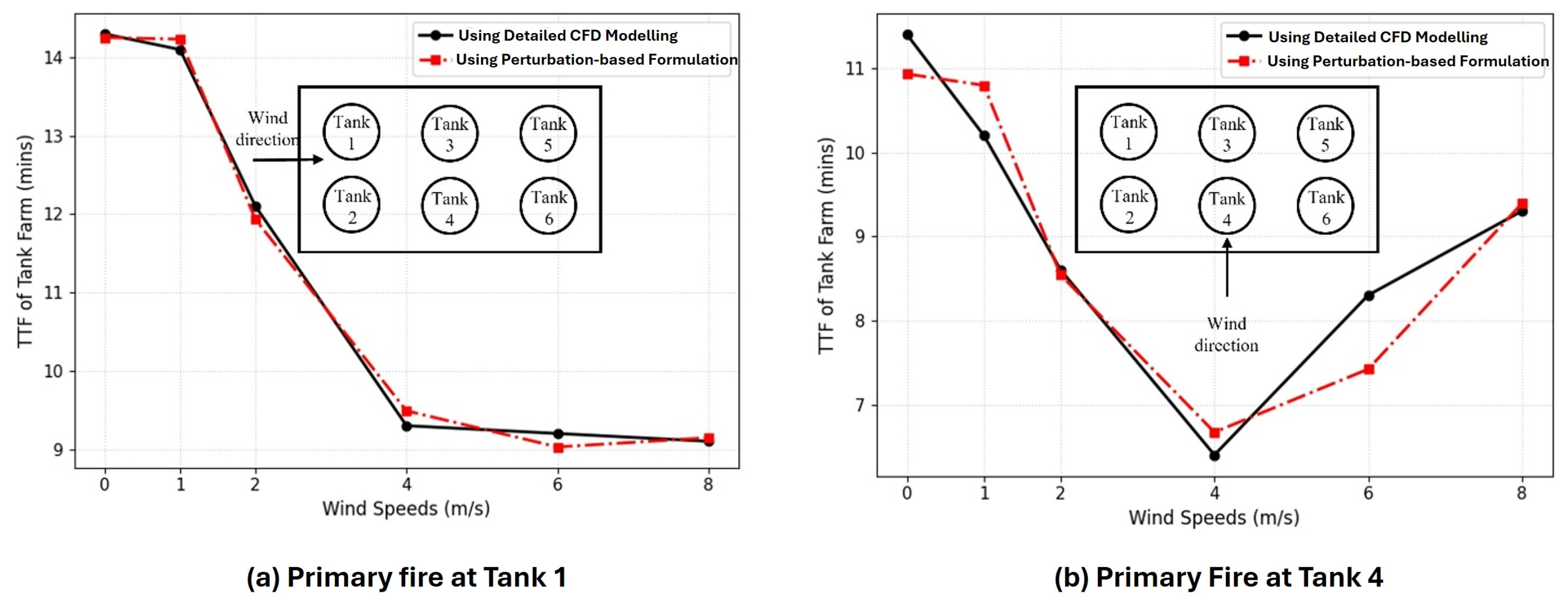
Figure 7 compares the tank farm TTFs obtained from the detailed CFD modelling-based calculation and proposed perturbation-based analytical formulation for primary fire scenarios initiated at Tanks 1 and 4 under varying wind conditions. For the primary fire initiated at Tank 1, as shown in Figure 7a, both calculations predicted a sharp reduction in the tank farm TTF with increasing wind speed, up to approximately 4 m/s. However, beyond 4 m/s, the tank farm TTF remained nearly constant despite further increases in the wind speed. This behaviour suggests that beyond 4 m/s, the domino propagation dynamics are fully dominated by a directional flame tilt toward the downwind tanks. Since the primary fire originated at Tank 1, located at the upper corner of the 2 × 3 tank matrix, increasing wind speed progressively channelled the incident heat flux toward a limited downwind propagation path. Once this directional alignment was fully established at around 4 m/s, further increases in wind speed yielded comparatively smaller changes in the overall TTF of the tank farm because the escalation path and dominant thermal interaction mechanism remained essentially unchanged.
A different trend was observed for the primary fire at Tank 4, as shown in Figure 7b. Similar to the Tank 1 scenario, increasing wind speed initially reduced the tank farm TTF because of intensified flame tilt on the downwind tanks. The minimum TTF of the tank farm occurred at approximately 4 m/s wind speed, after which the overall tank farm TTF began to increase slightly with further increases in wind speed. This behaviour indicates that 4 m/s again served as a critical transition point governing the domino escalation dynamics. However, unlike the corner-located Tank 1 scenario, the primary fire at Tank 4 was near the centre of the 2 × 3 tank matrix, leading to a fundamentally different spatial redistribution of incident heat flux under strong wind conditions. At moderate wind speeds, the directional flame tilt significantly accelerated the failure of the immediate downwind tanks, triggering a rapid domino effect. At higher wind speeds beyond 4 m/s, however, the intensified directional plume caused the offset Tanks 2 and 6 to experience approximately a 24% reduction in incident heat flux compared to the no-wind condition (Figure 5c). This reduced thermal exposure delayed their failure, shifting the final tank failure that governed the overall tank farm TTF toward the less-exposed tanks and resulting in an increase in tank farm TTF at higher wind speeds, despite the accelerated failure of the directly aligned downwind tanks (Figure 7b).
Figure 7 also shows that the tank farm TTFs obtained using the proposed perturbation-based analytical formulation are consistent with those obtained from the detailed CFD modelling-based calculation. A quantitative comparison is presented in Table 3, which lists the tank farm TTFs determined by both approaches for all considered wind speeds, along with the corresponding absolute and relative errors. For the primary fire scenarios at Tanks 1 and 4, the tank farm TTF using the perturbation-based formulation achieved mean absolute errors (MAEs) of 0.13 min and 0.40 min, respectively, corresponding to mean relative errors (MREs) of 1.2% and 4.5%. It is worth noting that, compared with the primary pool fire scenario at Tank 1, the relative errors were somewhat higher under the primary fire scenario at Tank 4, with one case at 6 m/s reaching 9.6%. This behaviour could be associated with the more complex multi-tank interactions that occurred when the primary fire was at Tank 4, where two offset tanks (Tanks 2 and 6) were adjacent to it. Under these conditions, the perturbation-based approximation shows slightly greater deviation from the TTF calculations obtained from detailed CFD modelling. Nevertheless, for the primary fire at Tank 4, the relative errors were below 6% in almost all other cases (as shown in Table 3), suggesting that this represents a localised deviation rather than a systematic limitation of the proposed formulation.
Overall, the tank farm TTF from the proposed analytical formulation yielded an MAE of only 0.26 min and an MRE of 2.8% across all primary fire scenarios and wind conditions investigated. These results quantitatively demonstrate the close agreement between the proposed perturbation-based analytical formulation and detailed CFD modelling-based calculation, confirming its viability as a computationally efficient approximation for estimating tank farm TTF under wind conditions.
The perturbation-based analytical formulation that led to the calculations shown in Table 3 is given by Equation (11).
T T F   t a n k   f a r m   w i n d = T T F   t a n k   f a r m   n o   w i n d + (   T T F   S e c   t a n k w i n d T T F   S e c   t a n k n o   w i n d ) + C
Here, ’ T T F   t a n k   f a r m   w i n d ’ and ‘ T T F   t a n k   f a r m   n o   w i n d ’ are the TTFs of the tank farm under wind and no-wind conditions. The TTF under the no-wind condition represents the initial solution. T T F   S e c   t a n k w i n d and ‘ T T F   S e c   t a n k n o   w i n d ’ are the TTFs of the secondary tank under wind and no-wind conditions, respectively (which is the first-order perturbative term). All the TTF terms in Equation (11) are in mins. ‘ C ’ is the higher-order regression perturbative term obtained using polynomial regression and is expressed in mins.
To further explain the implementation of Equation (11), consider the case of a primary fire at Tank 1 with wind blowing from west to east, as shown in Figure 2a. First, to establish the baseline tank farm TTF, a CFD simulation of fire propagation throughout the tank farm is performed under no-wind conditions. Then, CFD modelling is required only for the secondary tank that receives the highest thermal exposure from the primary fire under wind effects (Tank 3 in the present case). The resulting TTF of the secondary tank is then incorporated into Equation (11) to estimate the overall tank farm TTF. This eliminates the need to simulate the complete domino escalation sequence under each wind condition.
From a practical engineering perspective, the proposed methodology provides a computationally efficient framework for rapid TTF assessment of tank farms. Once the baseline tank farm TTF has been established under no-wind conditions, only the wind-influenced effects on the secondary tank need to be evaluated through CFD simulations. The TTF of the secondary tank and the ‘ C ’ value (which is only a function of wind speed), along with the baseline TTF of the tank farm, can be incorporated into the developed Equation (11) to estimate the overall TTF of the tank farm under varying wind conditions. This substantially reduces computational effort while maintaining good prediction accuracy, as demonstrated by the results presented above.
From an overall emergency planning standpoint, the proposed formulation enables rapid prediction of tank farm TTF under varying wind conditions, allowing critical escalation pathways and vulnerable tanks to be identified without performing computationally intensive CFD simulations. For instance, the results in Figure 7 indicate that wind speeds up to 4 m/s substantially reduced the tank farm TTF when the primary fires were at Tanks 1 and 4. This was because of enhanced flame tilt and increased thermal exposure of downwind tanks. Since complete tank farm failure can have catastrophic consequences, timely prediction of its TTF is essential to support response planning and mitigate escalation. Compared with performing CFD simulations for every scenario, the proposed perturbation-based approach substantially reduces computational time while providing rapid estimates of tank farm TTF. Such information can support the prioritisation of vulnerable tanks, allocation of firefighting resources, and assessment of the available intervention time during emergency situations.

4.4. Limitations and Future Directions

It should be noted that the proposed perturbation-based analytical approach, including the first-order perturbation term and regression correction term ( C ), was developed and calibrated for a specific tank farm layout. The investigated arrangement represents a commonly considered tank farm layout configuration, characterised by uniform (equidistant) tank spacing, which has frequently been adopted in previous fire-induced domino effect studies [24,83,84]; however, the functional form and applicability of the proposed formulation may not be assumed to be universal. The proposed framework, however, demonstrates its capability to reduce the number of required CFD simulations, indicating its potential applicability to other tank farm layouts. For different layouts and fuels, the same framework steps can be followed, but this may result in a different ‘ C ’ value based on the configuration. Therefore, future studies could investigate a wider range of tank arrangements and other specifications to further assess and enhance the applicability of the proposed formulation. Additionally, the selected wind directions provide a conservative basis for assessing fire-induced domino effects and are consistent with the wind directions considered in previous studies [27,31]. However, the influence of varying wind directions, including oblique conditions, may alter thermal interaction mechanisms and could be further investigated using CFD. Overall, although this study introduces a novel perspective for rapid tank farm TTF estimation, it should be regarded as an important step toward developing a framework that translates detailed CFD-based fire-induced domino effect behaviour under wind conditions into a simplified analytical formulation. Such a framework provides the foundation for extending rapid TTF assessment to other tank farm layouts.

5. Conclusions

This study modelled the influence of wind speeds on fire-induced domino escalation and tank farm TTF using FDS. The results demonstrated that wind strongly governs domino propagation dynamics by intensifying thermal radiation toward downwind in-line tanks while reducing exposure on offset tanks. Furthermore, a centrally located primary fire led to faster, more hazardous escalation due to simultaneous thermal interactions among neighbouring tanks. It was also found that under higher wind conditions, the accelerated reduction in the TTF of tanks substantially shortened the available emergency response window, potentially resulting in fire escalation before effective firefighting intervention could be initiated. However, transient fire simulations involving multiple tanks and varying wind conditions are computationally expensive, which may limit their practicality for rapid risk assessment. Therefore, as a first attempt to reduce the computational burden associated with numerous CFD simulations of the fire-induced domino effect, a perturbation-based analytical formulation for estimating the TTF of a tank farm under wind was proposed. The formulation combined the no-wind tank farm TTF (baseline solution) with the wind-influenced perturbative correction terms. The proposed perturbation-based analytical formulation showed very good agreement with the tank farm TTF obtained using detailed CFD modelling. From a practical perspective, the methodology provides a rapid model for assessing domino effects and planning emergency responses under wind conditions. Nevertheless, the proposed perturbation-based formulation is specific to the investigated tank farm configuration and wind conditions. Future research could extend its applicability to other layouts, pool fire fuels and diameters, and wind directions, which will require additional CFD simulations and recalibration of the first-order perturbation and regression terms to enhance its general applicability.

Author Contributions

Conceptualization, A.A.M., R.A.-W. and M.S.N.; methodology, A.A.M., M.S.N., and R.A.-W.; formal analysis, A.A.M. and M.S.N.; investigation, A.A.M., R.A.-W. and M.S.N.; writing—original draft preparation, A.A.M.; writing—review and editing, A.A.M., M.S.N., and R.A.-W.; supervision, M.S.N. and R.A.-W.; funding acquisition, R.A.-W. and M.S.N. All authors have read and agreed to the published version of the manuscript.

Funding

This research received no external funding.

Data Availability Statement

The data presented in this study are available on request from the corresponding author. The data are not publicly available due to privacy.

Acknowledgments

Authors would like to acknowledge the support provided by the Deanship of Scientific Research of the German Jordanian University (GJU)–Jordan. The German Jordanian University seed Grant Number (SATS 06/2018) funded equipment used in the current project.

Conflicts of Interest

The authors declare no conflicts of interest.

Abbreviations

CFDComputational Fluid Dynamics
TTFTime to Failure
FDSFire Dynamics Simulator
BNBayesian Network
MLMachine Learning
RTEradiation transport equation
MLRPUAmass loss rate per unit area
LESLarge Eddy Simulation
SGSsubgrid-scale
NFPANational Fire Protection Association
Wwest
Eeast
Ssouth
Nnorth
MAEmean absolute error
MREmean relative error

Nomenclature

ρ fluid density
u velocity vector of the fluid flow
t time
gradient operation
p pressure
τ i j viscous stress tensor
f body forces
. u divergence of the velocity field
h s sensible enthalpy
Q ˙ heat release rate
k thermal conductivity
T temperature
α species
J α species diffusion flux vector
q ˙ r radiative heat flux vector
Z mixture fraction
Y F fuel mass fraction
Y O oxygen mass fraction
Y O ambient oxygen mass fraction
Y F I fuel mass fraction in the fuel stream
s stoichiometric coefficient
I radiative intensity
I b blackbody intensity
x optical path of radiation propagation
k a grey gas absorption coefficient
z elevation
z o reference height
u ( z ) wind velocity at the elevation
u o wind velocity at the reference height
r power-law exponent
Lhorizontal distance of the heat flux device from pool fire centre
Ddiameter of the pool fire
d x grid size
D characteristic fire diameter
ρ a density of the ambient air
C p specific heat of the ambient air
T a temperature of the ambient air
g gravitational acceleration
i number of tanks exposed to primary pool fire
T T F i failure time of exposed tanks
I i incident heat flux of exposed tanks
V i tank volume
S current stage in the domino effect
S 1 previous stage in the domino effect
t i , r e s , S residual time of tank at current stage
I i , S incident heat flux in the current stage
I i , S 1 incident heat flux in the previous stage
t i , S 1 elapsed time of tank in the previous stage
t m i n i m u m   f a i l u r e , S 1 minimum time to fail of failed tank in the previous stage
T T F i , a c c u m u l a t e d , S accumulated TTF of tank in the current stage due to synergistic effects
C regression perturbative term
R2coefficient of determination
T T F   t a n k   f a r m   w i n d TTF of tank farm under wind condition
T T F   t a n k   f a r m   n o   w i n d TTF of tank farm under no-wind condition
T T F   S e c   t a n k w i n d TTF of the secondary tank under wind condition
T T F   S e c   t a n k n o   w i n d TTF of the secondary tank under no-wind condition

Appendix A

Figure A1. This figure presents regression fit evaluation of three functional forms: degree 1 (linear), 2 (quadratic), and 3 (cubic) for the regression perturbative term ( C ) as a function of wind speed, for both fire scenarios considered. (ac) Primary fire at Tank 1, showing degree 1, 2, and 3 polynomial fits, respectively. (df) Primary fire at Tank 4, showing degree 1, 2, and 3 polynomial fits, respectively.
Modelling 07 00168 g0a1
Quadratic (best fit) expression for the regression perturbative term ( C ) for:
Primary fire at Tank 1:
c = 0.01 × w i n d   s p e e d 2 + 0.069 × w i n d   s p e e d 0.046
Primary fire at Tank 4:
c = 0.09 × w i n d   s p e e d 2 0.125 × w i n d   s p e e d 0.47

References

  1. Mishra, K.B.; Wehrstedt, K.D.; Krebs, H. Lessons learned from recent fuel storage fires. Fuel Process. Technol. 2013, 107, 166–172. [Google Scholar] [CrossRef] [Scilit]
  2. Wang, B.; Zhu, Z. A brief report and analysis on the July 19, 2019, explosion in the Yima gasification plant in Sanmenxia, China. Process Saf. Prog. 2020, 39, 3–7. [Google Scholar] [CrossRef] [Scilit]
  3. CNN. Texas District Attorney Files Charges Against Chemical Plant for Its 4-Day Fire. 2019. Available online: https://edition.cnn.com/2019/04/29/us/deer-park-itc-plant-fire-charges/index.html (accessed on 20 March 2021).
  4. Reniers, G.; Cozzani, V. Features of Escalation Scenarios; Elsevier: Amsterdam, The Netherlands, 2013; ISBN 9780444543233. [Google Scholar]
  5. Ou, Y.; Zhou, J.; Reniers, G. Numerical simulation of domino effects of tank fires in terms of time to failure. Process Saf. Environ. Prot. 2025, 202, 107751. [Google Scholar] [CrossRef] [Scilit]
  6. Zhang, X.; Tang, M.; Ren, F.; Li, X.; Xu, W. An Improved Approach to Estimate the Time to Failure for Large Oil Tank in Pool-Fire-Induced Domino Effects by Stress Failure. J. Fail. Anal. Prev. 2022, 22, 1954–1964. [Google Scholar] [CrossRef] [Scilit]
  7. Zhang, M.; Zheng, F.; Chen, F.; Pan, W.; Mo, S. Propagation probability of domino effect based on analysis of accident chain in storage tank area. J. Loss Prev. Process Ind. 2019, 62, 103962. [Google Scholar] [CrossRef] [Scilit]
  8. Landucci, G.; Gubinelli, G.; Antonioni, G.; Cozzani, V. The assessment of the damage probability of storage tanks in domino events triggered by fire. Accid. Anal. Prev. 2009, 41, 1206–1215. [Google Scholar] [CrossRef] [Scilit] [PubMed]
  9. Amin, M.T.; Scarponi, G.E.; Cozzani, V.; Khan, F. Improved pool fire-initiated domino effect assessment in atmospheric tank farms using structural response. Reliab. Eng. Syst. Saf. 2024, 242, 109751. [Google Scholar] [CrossRef] [Scilit]
  10. Wu, Z.; Hou, L.; Wu, S.; Wu, X.; Liu, F. The time-to-failure assessment of large crude oil storage tank exposed to pool fire. Fire Saf. J. 2020, 117, 103192. [Google Scholar] [CrossRef] [Scilit]
  11. Khakzad, N. A Tutorial on Fire Domino Effect Modeling Using Bayesian Networks. Modelling 2021, 2, 240–258. [Google Scholar] [CrossRef] [Scilit]
  12. Yang, J.; Zhang, M.; Zuo, Y.; Cui, X.; Liang, C. Improved models of failure time for atmospheric tanks under the coupling effect of multiple pool fires. J. Loss Prev. Process Ind. 2023, 81, 104957. [Google Scholar] [CrossRef] [Scilit]
  13. Chen, C.; Reniers, G.; Zhang, L. An innovative methodology for quickly modeling the spatial-temporal evolution of domino accidents triggered by fire. J. Loss Prev. Process Ind. 2018, 54, 312–324. [Google Scholar] [CrossRef] [Scilit]
  14. TNO. PSG2: Methods for the Calculation of Physical Effects (Yellow Book); The State Secretary of Housing Spatial Planning and the Environment (VROM): The Hague, The Netherlands, 2005. [Google Scholar]
  15. Hurley, M.J.; Gottuk, D.; Hall, J.R.; Harada, K.; Kuligowski, E.; Puchovsky, M.; Torero, J.; Watts, J.M.; Wieczorek, C. SFPE Handbook of Fire Protection Engineering, 5th ed.; Springer: New York, NY, USA, 2016; pp. 1–3493. [Google Scholar] [CrossRef] [Scilit]
  16. Assael, M.J. Fires, Explosions and Toxic Gas Dispersions- Effects Calculation & Risk Analysis; CRC Press: Boca Raton, FL, USA, 2010; ISBN 9781439826751. [Google Scholar]
  17. Khakzad, N.; Amyotre, P.; Khan, F. Valerio Cozzani Domino Effect Analysis Using Bayesian Networks. Risk Anal. 2013, 33, 292–306. [Google Scholar] [CrossRef] [Scilit] [PubMed]
  18. Li, X.; Liu, W.; Chen, B.; Zhou, N.; Huang, W.; Liang, Y.; Yuan, X.; Li, Z. Domino Effect Risk Modeling and Analysis of Tank Area Accidents Based on Accident Chain and Multifactor Coupling. ACS Chem. Health Saf. 2025, 32, 413–425. [Google Scholar] [CrossRef] [Scilit]
  19. Dueñas Santana, J.A.; Orozco, J.L.; Furka, D.; Furka, S.; Boza Matos, Y.C.; Febles Lantigua, D.; González Miranda, A.; Barrera González, M.C. A new Fuzzy-Bayesian approach for the determination of failure probability due to thermal radiation in domino effect accidents. Eng. Fail. Anal. 2021, 120, 105106. [Google Scholar] [CrossRef] [Scilit]
  20. Kamil, M.Z.; Taleb-Berrouane, M.; Khan, F.; Ahmed, S. Dynamic domino effect risk assessment using Petri-nets. Process Saf. Environ. Prot. 2019, 124, 308–316. [Google Scholar] [CrossRef] [Scilit]
  21. Zhou, J.; Reniers, G. A matrix-based modeling and analysis approach for fire-induced domino effects. Process Saf. Environ. Prot. 2018, 116, 347–353. [Google Scholar] [CrossRef] [Scilit]
  22. Huang, W.; Chen, X.; Qin, Y. A simulation method for the dynamic evolution of domino accidents in chemical industrial parks. Process Saf. Environ. Prot. 2022, 168, 96–113. [Google Scholar] [CrossRef] [Scilit]
  23. Ding, L.; Khan, F.; Abbassi, R.; Ji, J. FSEM: An approach to model contribution of synergistic effect of fires for domino effects. Reliab. Eng. Syst. Saf. 2019, 189, 271–278. [Google Scholar] [CrossRef] [Scilit]
  24. Ding, L.; Khan, F.; Guo, X.; Ji, J. A novel approach to reduce fire-induced domino effect risk by leveraging loading/unloading demands in chemical industrial parks. Process Saf. Environ. Prot. 2021, 146, 610–619. [Google Scholar] [CrossRef] [Scilit]
  25. Beyler, C.L. Fire Hazard Calculations for Large, Open Hydrocarbon Fires. In SFPE Handbook of Fire Protection Engineering; Springer: New York, NY, USA, 2016; pp. 2591–2662. [Google Scholar]
  26. Sun, B.; Guo, K.; Pareek, V.K. Computational fluid dynamics simulation of LNG pool fire radiation for hazard analysis. J. Loss Prev. Process Ind. 2014, 29, 92–102. [Google Scholar] [CrossRef] [Scilit]
  27. Ahmadi, O.; Mortazavi, S.B.; Pasdarshahri, H.; Mohabadi, H.A. Consequence analysis of large-scale pool fire in oil storage terminal based on computational fluid dynamic (CFD). Process Saf. Environ. Prot. 2019, 123, 379–389. [Google Scholar] [CrossRef] [Scilit]
  28. Elhelw, M.; El-Shobaky, A.; Attia, A.; El-Maghlany, W.M. Advanced dynamic modeling study of fire and smoke of crude oil storage tanks. Process Saf. Environ. Prot. 2021, 146, 670–685. [Google Scholar] [CrossRef] [Scilit]
  29. Shojaei Mehr, R.; Mohammadian Bishe, E.; Farhanieh, B.; Afshin, H. Numerical Investigation of the Combined Effect of Terrain Slope and Wind Velocity on Fire Spread Rate in Natural Pastures. Modelling 2025, 6, 15. [Google Scholar] [CrossRef] [Scilit]
  30. Chen, C.; Reniers, G.; Khakzad, N. A thorough classification and discussion of approaches for modeling and managing domino effects in the process industries. Saf. Sci. 2020, 125, 104618. [Google Scholar] [CrossRef] [Scilit]
  31. Masum Jujuly, M.; Rahman, A.; Ahmed, S.; Khan, F. LNG pool fire simulation for domino effect analysis. Reliab. Eng. Syst. Saf. 2015, 143, 19–29. [Google Scholar] [CrossRef] [Scilit]
  32. Yang, R.; Khan, F.; Neto, E.T.; Rusli, R.; Ji, J. Could pool fire alone cause a domino effect? Reliab. Eng. Syst. Saf. 2020, 202, 106976. [Google Scholar] [CrossRef] [Scilit]
  33. Li, X.; Chen, G.; Huang, K.; Zeng, T.; Zhang, X.; Yang, P.; Xie, M. Consequence modeling and domino effects analysis of synergistic effect for pool fires based on computational fluid dynamic. Process Saf. Environ. Prot. 2021, 156, 340–360. [Google Scholar] [CrossRef] [Scilit]
  34. McGrattan, K.; Hostikka, S.; McDermott, R.; Floyd, J.; Weinschenk, C.; Overhold, K. Fire Dynamics Simulator (FDS) Reference Guide: Validation; National Institute of Standards and Technology Special Publication; U.S. Department of Commerce: Washington, DC, USA, 2019; Volume 3. [CrossRef] [Scilit]
  35. Malik, A.A.; Nasif, M.S.; Arshad, U.; Mokhtar, A.A.; Tohir, M.Z.M.; Al-Waked, R. Predictive Modelling of Wind-Influenced Dynamic Fire Spread Probability in Tank Farm Due to Domino Effect by Integrating Numerical Simulation with ANN. Fire 2023, 6, 85. [Google Scholar] [CrossRef] [Scilit]
  36. Malik, A.A.; Nasif, M.S.; Mokhtar, A.A.; Mohd Tohir, M.Z. Numerical investigation of the effect of weather conditions on the escalation and propagation of fire-induced domino effect. Process Saf. Prog. 2021, 40, 296–308. [Google Scholar] [CrossRef] [Scilit]
  37. Khan, Z.; Ding, L.; Ji, J.; Zhang, Y. Innovative machine learning-based prediction of time-to-failure and domino fire escalation in chemical storage tanks. Reliab. Eng. Syst. Saf. 2026, 277, 113094. [Google Scholar] [CrossRef] [Scilit]
  38. Tamascelli, N.; Scarponi, G.E.; Amin, M.T.; Sajid, Z.; Paltrinieri, N.; Khan, F.; Cozzani, V. A neural network approach to predict the time-to-failure of atmospheric tanks exposed to external fire. Reliab. Eng. Syst. Saf. 2024, 245, 109974. [Google Scholar] [CrossRef] [Scilit]
  39. Yu, H.; Li, M.; Cai, H. Approximating the stance map of the SLIP runner based on perturbation approach. In Proceedings of the 2012 IEEE International Conference on Robotics and Automation, Saint Paul, MN, USA, 14–18 May 2012; pp. 4197–4203. [Google Scholar]
  40. Chen, G.; Wei, N.; Yan, L.; Lu, H.; Li, J. Perturbation-based approximate analytic solutions to an articulated SLIP model for legged robots. Commun. Nonlinear Sci. Numer. Simul. 2023, 117, 106943. [Google Scholar] [CrossRef] [Scilit]
  41. Narisetti, R.K.; Leamy, M.J.; Ruzzene, M. A Perturbation Approach for Predicting Wave Propagation in One-Dimensional Nonlinear Periodic Structures. J. Vib. Acoust. 2010, 132, 031001. [Google Scholar] [CrossRef] [Scilit]
  42. Fang, L.; Leamy, M.J. A perturbation approach for predicting wave propagation at the spatial interface of linear and nonlinear one-dimensional lattice structures. Nonlinear Dyn. 2024, 112, 5015–5036. [Google Scholar] [CrossRef] [Scilit]
  43. Anaraki, J.R.; Usefi, H. A Feature Selection based on perturbation theory. Expert Syst. Appl. 2019, 127, 1–8. [Google Scholar] [CrossRef] [Scilit]
  44. Silva, E.G.; Júunior, D.S.D.O.; Cavalcanti, G.D.; de Mattos Neto, P.S. Improving the accuracy of intelligent forecasting models using the Perturbation Theory. In Proceedings of the 2018 International Joint Conference on Neural Networks (IJCNN), Rio de Janeiro, Brazil, 8–13 July 2018; pp. 1–7. [Google Scholar]
  45. Black, F.; Schulze, P.; Unger, B. Efficient Wildland Fire Simulation via Nonlinear Model Order Reduction. Fluids 2021, 6, 280. [Google Scholar] [CrossRef] [Scilit]
  46. Cheng, S.; Prentice, I.C.; Huang, Y.; Jin, Y.; Guo, Y.-K.; Arcucci, R. Data-driven surrogate model with latent data assimilation: Application to wildfire forecasting. J. Comput. Phys. 2022, 464, 111302. [Google Scholar] [CrossRef] [Scilit]
  47. Bilyaz, S.; Ezekoye, O.A. Fire Smoke Transport and Opacity Reduced-Order Model (Fire-STORM): A New Computer Model for High-Rise Fire Smoke Simulations. Fire Technol. 2019, 55, 981–1012. [Google Scholar] [CrossRef] [Scilit]
  48. McGrattan, K.; Hostikka, S.; McDermott, R.; Floyd, J.; Weinschenk, C.; Overhold, K.; McGrattan, K.; Hostikka, S.; McDermott, R.; Floyd, J.; et al. Sixth Edition Fire Dynamics Simulator User ’s Guide (FDS). NIST Spec. Publ. 2020, 1019, 1–339. [Google Scholar] [CrossRef] [Scilit]
  49. McGrattan, K.; Hostikka, S.; McDermott, R.; Floyd, J.; Weinschenk, C.; Overhold, K. Fire Dynamics Simulator technical reference guide: Mathematical model. Natl. Insitute Stand. Technol. 2019, 1, 201. [Google Scholar]
  50. Floyd, J.E.; McGrattan, K.B.; Hostikka, S.; Baum, H.R. CFD fire simulation using mixture fraction combustion and finite volume radiative heat transfer. J. Fire Prot. Eng. 2003, 13, 11–36. [Google Scholar] [CrossRef] [Scilit]
  51. Rengel, B.; Mata, C.; Pastor, E.; Casal, J.; Planas, E. A priori validation of CFD modelling of hydrocarbon pool fires. J. Loss Prev. Process Ind. 2018, 56, 18–31. [Google Scholar] [CrossRef] [Scilit]
  52. Fernandes, C.S.; Fraga, G.C.; França, F.H.R.; Centeno, F.R. Radiative transfer calculations in fire simulations: An assessment of different gray gas models using the software FDS. Fire Saf. J. 2021, 120, 103103. [Google Scholar] [CrossRef] [Scilit]
  53. Prasad, K.; Bova, A.; Whetstone, J.; Novakovskaia, E. Greenhouse Gas Emissions and Dispersion. 1. Optimum Placement of Gas Inlets on a Building Rooftop for the Measurement of Greenhouse Gas Concentrations, Special Publication (NIST SP); National Institute of Standards and Technology Special Publication; U.S. Department of Commerce: Washington, DC, USA, 2013. [CrossRef] [Scilit]
  54. Biswas, S.; Chen, J.S. Power Coefficient for Large Wind Turbines Considering Wind Gradient Along Height. Energies 2025, 18, 740. [Google Scholar] [CrossRef] [Scilit]
  55. Yamaguchi, T.; Wakasa, K. Oil Pool Fire Experiment. Fire Saf. Sci. 1986, 1, 911–918. [Google Scholar] [CrossRef] [Scilit]
  56. Miao, Y.; Chen, Y.; Delichatsios, M.A.; Lin, Y.; Hu, L. Crosswise heat flux and temperature profiles over downstream surface of gas-fueled pool fires in relatively strong wind. Int. J. Heat Mass Transf. 2024, 228, 125569. [Google Scholar] [CrossRef] [Scilit]
  57. Lu, X.; Ren, N.; Xiong, G.; Krisman, A.; Gaurav, A.; Yoshioka, H.; Nishio, Y.; Noguchi, T.; Wang, Y. A numerical study of transport phenomena and radiation transfer in compartment and façade fires. Fire Saf. J. 2025, 158, 104556. [Google Scholar] [CrossRef] [Scilit]
  58. Ellzey, J.L.; Berbe, J.G.; Tay, E.Z.F.; Foster, D.E. Total Soot Yield from a Propane Diffusion Flame in Cross-Flow. Combust. Sci. Technol. 1990, 71, 41–52. [Google Scholar] [CrossRef] [Scilit]
  59. Kunhyuk, S.; Ryan, F.; Bundy, M.; Marco, F.; Anthony, H. The Global and Local Structure of Medium-Scale Pool Fires (NIST TN 2162), National Institute of Standards and Technology; National Institute of Standards and Technology: Gaithersburg, MD, USA, 2024.
  60. Lin, C.H.; Ferng, Y.M.; Hsu, W.S.; Pei, B.S. Investigations on the characteristics of radiative heat transfer in liquid pool fires. Fire Technol. 2010, 46, 321–345. [Google Scholar] [CrossRef] [Scilit]
  61. McDermott, R. Taming the Dragon: Ten milestones in FDS development. In Proceedings of the Eighth International Seminar on Fire and Explosion Hazards (ISFEH8), Hefei, China, 25–28 April 2016; pp. 3–11. [Google Scholar]
  62. McGrattan, K.; Miles, S. Modeling Fires Using Computational Fluid Dynamics (CFD). In SFPE Handbook of Fire Protection Engineering; Hurley, M.J., Gottuk, D., Hall, J.R., Harada, K., Kuligowski, E., Puchovsky, M., Torero, J., Watts, J.M., Wieczorek, C., Eds.; Springer: New York, NY, USA, 2016; pp. 1034–1065. ISBN 978-1-4939-2565-0. [Google Scholar]
  63. Wickström, U. SFPE Handbook of Fire Protection Engineering-Methods for Predicting Temperatures in Fire-Exposed Structures, 5th ed.; Springer: New York, NY, USA, 2016; ISBN 9781493925650. [Google Scholar]
  64. Philip, J.D. SFPE Handbook of Fire Protection Engineering, 3rd ed.; National Fire Protection Association: Quincy, MA, USA, 2002. [Google Scholar]
  65. Hasnain, S.A.; Nasif, M.S.; Pao, W.; Al-Waked, R. Numerical investigation of smoke contamination in atrium upper balconies at different down stand depths. Build. Simul. 2016, 10, 365–381. [Google Scholar] [CrossRef] [Scilit]
  66. González-Alvear, M.; Lázaro, M.; Daniel, A.; Morgado, E.; Miguel, Á.J.; Lázaro, D. Effect of FDS uncertainty in fire simulations of nuclear power plants under different ventilation conditions. Nucl. Eng. Des. 2026, 449, 114733. [Google Scholar] [CrossRef] [Scilit]
  67. Zhou, J.; Reniers, G. Analysis of emergency response actions for preventing fire-induced domino effects based on an approach of reversed fuzzy Petri-net. J. Loss Prev. Process Ind. 2017, 47, 169–173. [Google Scholar] [CrossRef] [Scilit]
  68. York, N.; Metro, C. NFPA 30-2008: Basic Requirements for Storage Tanks; Society of Fire Protection Engineers: New York, NY, USA, 2011. [Google Scholar]
  69. Vannak, D.; Liew, M.S.; Yew, G.Z. Time Domain and Frequency Domain Analyses of Measured Metocean Data for Malaysian. Int. J. Geol. Environ. Eng. 2013, 7, 549–554. [Google Scholar]
  70. Goddard, K.A. Investigation of Wind Patterns on Marion Island Using Computational Fluid Dynamics and Measured Data. Master’s Thesis, University of Pretoria, Pretoria, South Africa, 2021. [Google Scholar]
  71. Drysdale, D.D. Ignition of liquids. In SFPE Handbook of Fire Protection Engineering, Fifth Edition; Springer: New York, NY, USA, 2016; pp. 554–580. ISBN 9781493925650. [Google Scholar]
  72. Cozzani, V.; Gubinelli, G.; Antonioni, G.; Spadoni, G.; Zanelli, S. The assessment of risk caused by domino effect in quantitative area risk analysis. J. Hazard. Mater. 2005, 127, 14–30. [Google Scholar] [CrossRef] [Scilit] [PubMed]
  73. Chen, C.; Reniers, G.; Khakzad, N. Integrating safety and security resources to protect chemical industrial parks from man-made domino effects: A dynamic graph approach. Reliab. Eng. Syst. Saf. 2019, 191, 106470. [Google Scholar] [CrossRef] [Scilit]
  74. Lipponen, A.; Huttunen, J.M.J.; Romakkaniemi, S.; Kokkola, H.; Kolehmainen, V. Correction Of Model Reduction Errors In Simulations. J. Comput. Methods Sci. Eng. 2018, 40, 305–327. [Google Scholar] [CrossRef] [Scilit]
  75. Murdock, J.A. Perturbations Theory and Methods; Society for Industrial and Applied Mathematics: Philadelphia, PA, USA, 1999. [Google Scholar]
  76. Gaeta, G. Perturbation Theory: Mathematics, Methods and Applications. A Volume in the Encyclopedia of Complexity and Systems Science, 2nd ed.; Meyers, R.A., Ed.; Springer: New York, NY, USA, 2022; ISBN 9781071626207. [Google Scholar]
  77. Hirschfelder, J.; Brown, W.B.; Epstein, S.T. Recent Developments in Perturbation Theory. Adv. Quantum Chem. 1964, 1, 255–374. [Google Scholar] [CrossRef] [Scilit]
  78. Zwiebach, B. Chapter 1: Perturbation Theory. In 8.06 Quantum Physics III, Spring 2018. MIT OpenCourseWare. 2018. Available online: https://ocw.mit.edu/courses/8-06-quantum-physics-iii-spring-2018/ (accessed on 15 June 2026).
  79. Zhou, J.; Reniers, G. Petri net simulation of multi-department emergency response to avert domino effects in chemical industry accidents. Process Saf. Environ. Prot. 2021, 146, 916–926. [Google Scholar] [CrossRef] [Scilit]
  80. National Fire Protection Association. NFPA 1710: Standard for the Organization and Deployment of Fire Suppression Operations, Emergency Medical Operations, and Special Operations to the Public by Career Fire Departments; National Fire Protection Association: Quincy, MA, USA, 2020. [Google Scholar]
  81. Jianfeng, Z.; Reniers, G. Probabilistic Petri-net addition enabling decision making depending on situational change: The case of emergency response to fuel tank farm fire. Reliab. Eng. Syst. Saf. 2020, 200, 106880. [Google Scholar] [CrossRef] [Scilit]
  82. Bujang, Z.; Ibrani, M.; Adam, S.; Adam, M.; Marzuki, O.F.; Kamarudin, S. Industrial Fire Brigade Emergency Response Time Parameters for Oil & Gas Facility. Int. J. Acad. Res. Bus. Soc. Sci. 2023, 13, 134–152. [Google Scholar] [CrossRef] [Scilit] [PubMed]
  83. Khakzad, N.; Khan, F.; Amyotte, P.; Cozzani, V. Risk Management of Domino Effects Considering Dynamic Consequence Analysis. Risk Anal. 2014, 34, 1128–1138. [Google Scholar] [CrossRef] [Scilit] [PubMed]
  84. Zhou, J.; Reniers, G.; Cozzani, V. Improved probit models to assess equipment failure caused by domino effect accounting for dynamic and synergistic effects of multiple fires. Process Saf. Environ. Prot. 2021, 154, 306–314. [Google Scholar] [CrossRef] [Scilit]
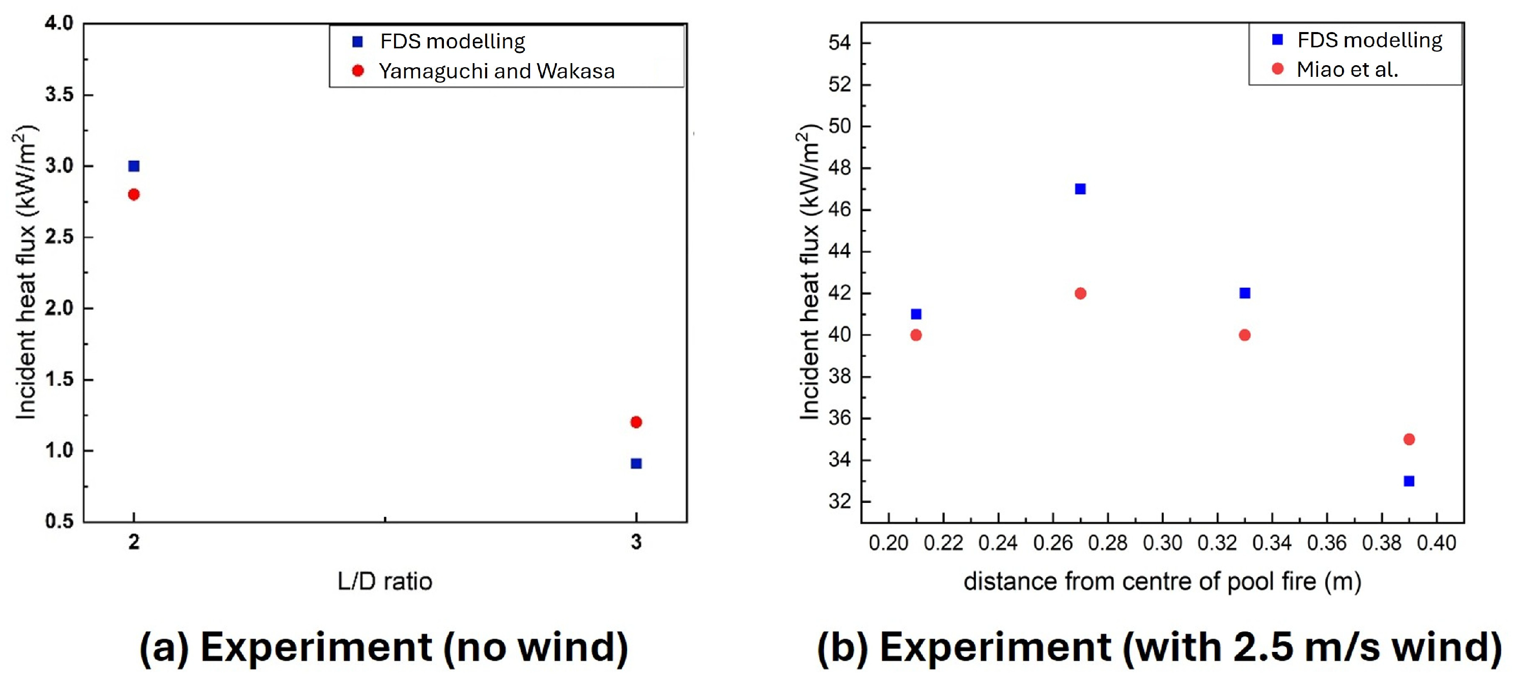
Figure 1. FDS modelling validation against experimental studies: (a) experiment (no wind) by Yamaguchi and Wakasa [55], (b) experiment (with 2.5 m/s wind) by Miao et al. [56].
Modelling 07 00168 g001
Figure 2. Depiction of (a) the tank farm layout and wind direction scenarios considered for the domino effect escalation analysis, and (b) the mesh independence study.
Modelling 07 00168 g002
Figure 3. Quadratic regression fit of the regression perturbative term ( C ) as a function of wind speed ranging from 0 to 8 m/s for: (a) primary fire scenario at Tank 1 (R2 = 0.904), and (b) primary fire scenario at Tank 4 (R2 = 0.937).
Modelling 07 00168 g003
Figure 4. Spatial contours of incident heat flux during domino evolution stages obtained from FDS for the primary fire at Tank 1, shown for selected wind speeds of (a) no wind, (b) 4 m/s, and (c) 8 m/s.
Modelling 07 00168 g004
Figure 5. Spatial contours of incident heat flux during domino evolution stages obtained from FDS for the primary fire at Tank 4, shown for selected wind speeds of (a) no wind, (b) 4 m/s, and (c) 8 m/s.
Modelling 07 00168 g005
Figure 6. Escalation path and respective accumulated Time to Failure (TTFs) of tanks in the domino escalation process obtained from detailed Computational Fluid Dynamics (CFD) modelling-based calculations, with primary fire at Tank 1, shown for (a) no wind, (b) 4 m/s, and (c) 8 m/s, and with primary fire at Tank 4 under (d) no wind, (e) 4 m/s, and (f) 8 m/s. The shades represent domino evolution stages (darkest is the primary tank on fire, and the lightest is the last tank in the evolution).
Modelling 07 00168 g006
Figure 7. TTF of tank farm calculated by detailed CFD modelling-based calculation and proposed perturbation-based analytical formulation under varying wind speeds, for (a) primary fire at Tank 1 and (b) primary fire at Tank 4.
Modelling 07 00168 g007
Table 3. Error analysis and validation of the tank farm TTF obtained by perturbation-based analytical formulation against the one obtained by detailed CFD modelling across different wind speeds for primary fires initiated at Tanks 1 and 4.
Wind Speeds (m/s)TTF Detailed CFD Modelling (mins)TTF Perturbation-Based (mins)Absolute Error (mins)Relative Error (%)
Primary fire at Tank 1014.314.20.10.7
114.114.20.10.7
212.111.90.21.6
49.39.50.22.1
69.29.00.22.2
89.19.10.00.0
Mean Error 0.131.2
Primary fire at Tank 4011.410.90.54.4
110.210.80.65.9
28.68.50.11.2
46.46.70.34.7
68.37.50.89.6
89.39.40.11.1
Mean Error 0.44.5
Disclaimer/Publisher’s Note: The statements, opinions and data contained in all publications are solely those of the individual author(s) and contributor(s) and not of MDPI and/or the editor(s). MDPI and/or the editor(s) disclaim responsibility for any injury to people or property resulting from any ideas, methods, instructions or products referred to in the content.