Optimal Item Placement for Information Retrieval in Stochastic Paired Comparison Models Under Special Comparison Structures

Abstract

Paired comparison models are examined from the perspective of the placement of objects within specific comparison structures. For both pairwise comparison matrix-based models and stochastic models, previous studies have examined which comparison structures maximize the amount of information that can be recovered from incomplete comparisons. In this paper, we investigate how the amount of extracted information can be increased in stochastic paired comparison models—primarily the Bradley–Terry model—by way of exploiting prior information about the ranking of the objects, if such information is available. We examine several comparison structures to identify the optimal placement of objects within each structure with respect to information recovery and evaluability. The investigated structures are the star graph, the union of two star graphs, and the union of two edge-disjoint spanning trees. Parameters are estimated using the maximum likelihood method. The applied evaluation metrics are the Euclidean distance, Pearson, Spearman, and Kendall correlations, called similarity metrics. Moreover, the rate of evaluable datasets and an inconsistency index is also computed. We found that, in almost all cases, all four similarity metrics identified the same placement as optimal. Our results show that, for the star graph, placing an object of medium strength at the center and comparing all other object to it maximizes the amount of information recovered from the comparisons. For the union of two star graphs, placing objects that occupy middle positions in the ranking at the centers also outperforms the commonly used best–worst centered placement. However, the union of two edge-disjoint spanning trees provides, on average, even better information recovery based on all investigated metrics. We also examined the proportion of evaluable datasets and found it to be higher when medium-strength objects were placed at the centers. Finally, we compared the findings obtained from the stochastic models with those from pairwise comparison matrix-based models and observed strong agreement between the two approaches.

1. Introduction

Information retrieval is becoming increasingly important in our daily lives. There is hardly a moment during the day when we do not use AI solutions [1]. These models perform extremely well with large amounts of data, but when the amount of data is limited, overfitting and instability result in serious challenges [2,3]. Therefore, it is often recommended to rely on other solutions [4,5].

Pairwise comparison models perform excellently even with limited available information [6,7,8]. Comparison in pairs is a commonly used and established approach for information retrieval when there is a high degree of uncertainty in characterizing objects using scale values. Several models and evaluation methods are available; the two main families are the pairwise comparison matrices (PCM)-based models [9,10] and models with stochastic background. This latter family contains the general Thurstone-motivated models [11,12], and the Bradley–Terry models, as special cases [13,14].

In pairwise comparison models, the data are derived by comparing two objects with one another, rather than against a scale. In many cases, where it is very difficult to relate the object from some perspective to a predefined scale, comparing objects to one another is an excellent approach; as the data become more reliable: the subjective element inherent in the interpretation of the scale values is thereby removed.

Efficiency and consistency play crucial roles in information retrieval where it is very costly to perform a comparison, or where only a very small number of comparisons can be made (for example, in sports tournaments, where the matches themselves are considered comparisons). If the results of the comparisons are consistent, any and all information is recoverable from any incomplete evaluable dataset [9,15]. However, this is not the case when the dataset is inconsistent.

A great deal of research has focused on optimal comparison structures for PCMs, such as which structures perform better given the same number of comparison edges. There are numerous articles on the optimal structure of comparison graphs and their analysis [16,17,18,19,20]. These studies demonstrate that highly effective information retrieval can be achieved using small amounts of well-designed and collected pairwise comparison data. In many cases, when the comparisons are incomplete, it is either impossible or not worthwhile to provide the missing comparisons. In their article, Bozóki et al. [20] explore this topic to determine how to retrieve as much information as possible, when a comparison matrix is incomplete. This research found that it is indeed worthwhile to use appropriate comparison structures to achieve better information retrieval. The study shows that as the number of comparisons increases, so does the amount of information that can be retrieved; however, when the number of comparisons remains the same, it is advisable to use certain structures. In the case of two-option Thurstone-motivated models, as well as the Davidson model, we found that the optimal comparison structures are the same as those for PCMs [15,21]. Therefore, the conclusions regarding the optimal comparison structures are the same as in the case of PCM-based models. An important finding of the publications [15,20] is that even when more pairs are compared, a poorly designed comparison structure may result in less effective information retrieval than an optimal comparison structure with fewer comparisons. Within the family of stochastic models, other researchers have also addressed the design of optimal comparisons for the two-option Bradley–Terry model [22,23,24]. These studies investigated the question of which objects should be compared, so as to require the least amount possible, while still allowing the greatest possible amount of information to be retrived from them. These publications are based on the D-optimality criterion and demonstrate that highly efficient information extraction can be achieved even with a small number of well-designed comparisons. In the case of a large number of objects, Jiang et al. [25] proposed an algorithm that can be used to design an optimal comparison structure.

When the number of comparisons is minimized while still ensuring an evaluable dataset—that is, when the number of comparisons equals the number of objects minus one—the star graph comparison structure was found to be optimal for both PCM-based and Thurstone-motivated models. This conclusion is published in [15]. The question arises: by fixing the number of compared pairs, applying the optimal comparison structure, would it be possible to further increase the efficiency of information retrieval by designing comparisons within the structure—specifically, by comparing certain objects with other objects. In multi-criteria decision-making, comparisons between objects and the best (highest-strength) and worst (lowest-strength) objects, as used in the Best-Worst Method (BWM), are widely applied. Numerous articles address this topic [17,26,27,28,29,30]. In many respects, this method offers an excellent approach, as it makes it one of the easiest ways to ensure consistency and eliminate inconsistencies within the results of the comparisons. Furthermore, the impact of any subjective errors made by the evaluator is significantly reduced due to the substantial dissimilarities between the strength ratings. This method is likewise used in [29]. Naturally, this assumes some prior knowledge regarding the ranking of the objects; however, identifying the strongest and the weakest is can be considered simplest task. Another solution is the method of comparing the best and second best (TOP2) ratings, as described in [19]. Applying these objects’ placement, most of the objects are compared to two other objects, with only two exceptions: the best and the worst or the second best.

The former observations show that it is worth comparing the objects in approximately equal numbers [31]; therefore, the use of quasi-regular graph structures is also common [16]. The only exception is the case of the spanning tree: here the star graph structure is optimal for information extraction, in average.

In the case of comparisons in pairs, regarding optimal structures, it has previously been investigated only for PCMs [19,26,29,30] whether, if ordinal information about the objects is available, their specific placement within the given structure can further improve information retrieval. In this article, we investigate optimal objects’ placement within the context of Thurstone-motivated models, namely how objects can be optimally placed within a comparison structure to maximize information retrieval. Besides the simplest star graph structure, we focus on the structures previously considered for PCMs in [19], i.e., the union of two star graphs structure and the union of two edge-disjoint spanning trees. We not only examine whether the results also hold true for Thurstone-motivated models, such as that TOP2 centered comparisons are superior to best-worst comparisons, but also systematically investigate whether a comparison to the best or the worst is the best possible option, or whether a comparison to an intermediate object-pair is more beneficial. Based on our intuition, the relative positions of objects with respect to intermediate strength objects provide more information about the objects than their positions with respect to extreme objects, despite the fact that the latter approach is expected to result in a more consistent dataset. Although the comparisons with extreme objects is the usual scenario, it is worth investigating whether it would be worth selecting intermediate strength objects as the center, instead of extremes. This issue has not yet been explored in the context of stochastic models; furthermore, this research takes a much wider approach—using several structures—to determine which comparison strategy is more effective for information retrieval, data consistency, and providing a greater proportion of evaluable datasets compared to the ones examined in previous studies. The method of investigation is computer simulation based on a large number of simulations. Out of the Thurstone-motivated models, we will mainly apply the Bradley–Terry model [13] in our work, partly because this model is widely used, and partly because it is exceptionally well-suited for performing large-scale simulations [32].

The structure of this article is as follows: in Section 2, we present the model we used; in Section 3 we detail the simulation method we applied; and in Section 4, we present the results of the simulations. In Section 5, we discuss the simulation results. Finally, in Section 6, we summarize our findings, and we raise further directions and questions.

2. The Investigated Model

In the stochastic paired comparison models, it is assumed that the current strength of an object can be well described by a random variable which are behind the objects’ performances. Thurstone presented his model in 1927, in his article [11]. The (average) strength of each object to be compared is the expected value of its latent random variable. The ordering of the expected values determines the rank positions of the objects.

Let there be n objects; we denote the random variable of the i-th object by ${\xi }_i$, while its expectation is denoted by $m_i$, $i=1,\cdots ,n$. In the original Thurstone model, the random variables followed Gaussian distribution. Here, we apply a general model, called Thurstone-motivated model, in which the distribution function of the differences of the latent random variable is general. The cumulative distribution function (c.d.f.) F satisfies the property $0<F\left(x\right)<1$, it is three times continuously differentiable, moreover, the probability density function $f\left(x\right)=F^{\prime }\left(x\right)$ is symmetric about 0 and is strictly log-concave. A special case is the Bradley–Terry model, when $F\left(x\right)$ is the logistic c.d.f.

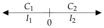
In this paper we apply two-option models. When comparing objects i and j in a two-option model, two options, better and worse are allowed in decisions: i is better than j or i is worse than j according to a decision. Naturally, if i is better than j according to a decision, then this same decision means that j is worse than i. The decision is determined by the difference of the current values of the latent random variables: we compare the difference with zero. We assign intervals to each decision; see Figure 1. Decision $C_1$ is the worse one, to which $I_1=(-\infty ;0)$ is associated, while decision $C_2$ is the better one, to which $I_2=[0;+\infty )$ is associated.

Since

$${\xi }_i-{\xi }_j=m_i-m_j+{\eta }_{i,j},i=1,...,n,j=1,...,n,i\ne j,$$

(1)

where ${\eta }_{i,j}$ are supposed to be identically distributed random variables with c.d.f. F, the probability that i is worse than j is as follows:

$$p_{i,j,1}=P({\xi }_i-{\xi }_j<0)=F(m_j-m_i),$$

(2)

while the probability that i is better than j is

$$p_{i,j,2}=P(0\le {\xi }_i-{\xi }_j)=F(m_i-m_j).$$

(3)

Equations (2) and (3) depend only on the differences between the expected values. We need to estimate the strength of the objects, i.e., the expectations of the random variables. For this purpose we use the maximum likelihood estimation (MLE) method. Assuming independent decisions, the likelihood function is

$$L\left(A\right|m_1,\dots ,m_n)={\displaystyle \prod _{k=1}^2}{\displaystyle \prod _{i=1}^{n-1}}{\displaystyle \prod _{j=i+1}^n}{p}_{i,j,k}^{A_{i,j,k}},$$

(4)

where $A_{i,j,k}$ denotes the number of times the k-th decision ($k=1,2$) was made during the comparisons of objects i and j, and $k=1$ corresponds to the decision worse, while $k=2$ corresponds to the decision better. For example, $A_{1,2,2}=5$ means that, when comparing the first and second objects, the first object was better than the second object on five occasions. Taking the logarithm of the likelihood function is beneficial, because this transforms the exponents into multiplication factors, and the multiplications into additions; although the maximum value of the function will change, its argument remains the same. The log-likelihood function is

$$\log L\left(A\right|m_1,m_2,\dots ,m_n)={\displaystyle \sum _{k=1}^2}{\displaystyle \sum _{i=1}^{n-1}}{\displaystyle \sum _{j=i+1}^n}{A}_{i,j,k}·\log \left(p_{i,j,k}\right).$$

(5)

The maximum likelihood estimation of the parameter vector $\underline{m}=(m_1,\cdots ,m_n)$ is the argument of the maximum of (4) or (5), i.e.,

$$\widehat{\underline{m}}=\underset{\underline{m}\in {\mathbb{R}}^n,m_1=0}{\arg \max }\log L\left(A\right|\underline{m}).$$

(6)

The constraint $m_1=0$ does not affect the values of (4) and (5), since (2) and (3) depend only on the differences between the expectations. However, it is crucial for the uniqueness of the maximizer.

If the specified comparison results satisfy certain condition (see Theorem 1), then the maximum is attained and its argument is unique. This means that estimated strengths and rankings can be obtained via MLE. We will refer to such data as evaluable. To present these conditions we need the following definitions:

Definition 1

(directed graph of comparison data). Let the graph of comparison data $\overrightarrow{G}\left(A\right)$ be defined as follows: the vertices are the objects $1,\cdots ,n$, and there is a directed edge from i to j (i $\to j$), if $0<A_{i,j,2}$.

The necessary and sufficient condition for the evaluability of the data is as follows:

Theorem 1

([33]). Dataset $A=\left(A_{i,j,k}\right)$$i=1,\cdots ,n$, $j=1,\cdots ,n$, $k=1,2$ is evaluable if and only if the directed graph $\overrightarrow{G}\left(A\right)$ is strongly connected.

Remark 1.

In the case of a star graph structure, the condition for data evaluability is equivalent to the requirement that, for every compared pair, there exists at least one “worse” and one “better” decision between the objects.

During the simulations we generally use the Bradley–Terry model, as the numerical computations can be performed quickly using this model. In this case the c.d.f. of the differences is the logistic c.d.f., i.e.,

$$F\left(x\right)={\displaystyle \frac{1}{1+e^{-x}}},x\in \mathbb{R}.$$

(7)

We note, that in the case of the two-option Bradly-Terry model, the sufficient and necessary condition for data evaluability was proved in [34]. Although the model was published many years ago, it continues to be studied and has been linked to artificial intelligence [35,36,37].

Although the evaluability of the data depends on the data themselves, for planning the comparison structure it is useful the following graph definition:

Definition 2

(undirected graph of comparisons). The graph of comparisons $G\left(A\right)$ is defined as follows: let the vertices be the objects $1,\cdots ,n$. Let two objects, i and j, are connected by an undirected edge ($i-j$), if there is at least one comparison between them, i.e., $0<A_{i,j,1}+A_{i,j,2}$.

Remark 2.

It is straightforward to see that the strict connectivity of $\overrightarrow{G}\left(A\right)$ implies the connectivity of $G\left(A\right)$, but the converse does not hold. If $G\left(A\right)$ is not connected, then the dataset is not evaluable. It may not attain a maximum, and whenever the maximum is attained, it is attained by several parameter vectors.

3. Method of Investigation: Computer Simulation

Generally it is not possible to analytically determine the argument of the maximal value of the functions (4) and (5); therefore, numerical methods have to be applied. Consequently, we cannot state analytical results for the optimal objects’ placements.

Nevertheless, we can utilize a Monte Carlo simulation. This technique is widely used in various fields of research [38,39,40], including pairwise comparison methods [15,19,31,41].

The steps of the simulation are as follows:

1.

Let us fix the vector of objects’ strengths $\underline{m}=(m_1,\cdots ,m_n)$, alternatively, these coordinates have to be randomly generated. For fixed values, we use $m_i=(i-1)·d$, where $i=1,\dots ,n$. The value of $0<d$ is changed to simulate situations in which the strengths are close to each other, as well as and situations in which they differ substantially. If the coordinates are random, they are uniformly distributed on the interval [0, 3.5], follow Gaussian distribution before being sorted in ascending order, or they satisfy the requirements of the different situations. These coordinates are referred to as the original (or initial) parameters.

2.

Based on the strengths, for each $(i,j)$ pair we compute the probabilities $p_{i,j,k}$, $(k=1,2)$, applying Formulas (2) and (3).

3.

For each $(i,j)$$i<j$ pair, based on $p_{i,j,k}$, values, we generate l comparison results as follows. For each comparison, we generate a random number uniformly distributed on the interval $(0,1)$. If this number is smaller than $p_{i,j,1}$ then the outcome of that comparison is the decision “i is worse than j”. If the generated number is at least $p_{i,j,1}$, then the outcome of the comparison is the decision “i is better than j”. By counting how many times the outcomes of the comparisons resulted in “worse” and “better” decisions, we obtain data $A_{i,j,1}^{\left(C\right)}$ and $A_{i,j,2}^{\left(C\right)}$, respectively. Due to the symmetry, $A_{i,j,1}^{\left(C\right)}=A_{j,i,2}^{\left(C\right)}$. This procedure yields a random data matrix $A^{\left(C\right)}$, where the superscript C refers to the completeness of the data matrix.

4.

We omit the data $A_{i,j,1}^{\left(C\right)}$ and $A_{i,j,2}^{\left(C\right)}$ values from the dataset for all pairs that are not part of the comparison structure under consideration. The resulting incomplete data matrix is denoted by $A^{\left(S_I\right)}$. (The superscript $S_I$ refers to it being an incomplete comparison structure.) For example, if the comparison structure is a star graph with object i as its center, then the set of compared pairs is $\left\{\right(1,i),(2,i),\cdots ,(i-1,i),(i,i+1),\cdots ,(i,n\left)\right\}$. We only keep the data that corresponds to these pairs. All other data are considered zero for the incomplete cases.

5.

We investigate whether the dataset $A^{\left(S_I\right)}$ is evaluable or not by investigating whether the directed graph $\overrightarrow{G}\left(A^{\left(S_I\right)}\right)$ is strongly connected or not. If they are, we perform the maximum likelihood estimation. To do this, we use the fixed-point iteration solver, for which the stopping criterion is as follows: within the last 50 iterations, there has been no change to any parameter to within five decimal places.

6.

We compare the estimated parameter vector ${\underline{\widehat{m}}}^{\left(S_I\right)}$ obtained from each the objects’ placement under the investigated comparison structure with the original strengths by several metrics.

7.

We repeat Steps 1–6 for the specified number of simulations. For each investigated objects’ placement under the investigated structure, we count the rate of evaluable cases. For the evaluable cases we calculate the average of the computed metrics.

8.

We choose the optimal objects’ placement under the investigated structure, i.e., the one with the smallest or largest distances, respectively. Since the number of the objects’ placement is finite, a polynomial function of the number of objects, (for example $n-1$ in case of star graph), this can be performed easily.

The extent of information recovery can be described using various metrics. In our research, we used the following four commonly applied metrics to compare the original and the estimated strength parameters and rankings.

• One can investigate the distance between the original and the estimated strengths based on the data set. For this we used the Euclidean distance as an objective function to optimize.
  Euclidean distance:

  $$D(\underline{m},{\underline{\widehat{m}}}^{\left(S_I\right)})=\sqrt{\sum _{i=1}^n{(m_i-{\widehat{m}}_i^{\left(S_I\right)})}^2}.$$

  (8)
• We can also consider their correlation as another objective function for optimization.
  Pearson’s correlation [42]:

  $$CORR(\underline{m},{\underline{\widehat{m}}}^{\left(S_I\right)})={\displaystyle \frac{\frac{{\sum }_{i=1}^n{m}_i·{\widehat{m}}_i^{\left(S_I\right)}}{n}-\underline{\overline{m}}·{\underline{\overline{\widehat{m}}}}^{\left(S_I\right)}}{\sqrt{\frac{{\sum }_{i=1}^n{\left(m_i-\underline{\overline{m}}\right)}^2}{n}}·\sqrt{\frac{{\sum }_{i=1}^n{\left(m_i^{\left(S_I\right)}-{\overline{\underline{\widehat{m}}}}^{\left(S_I\right)}\right)}^2}{n}}}},$$

  (9)
• The distances between the strength parameters are not the only quantities worth investigating; differences between rankings can also provide valuable information from the perspective of information retrieval. Therefore, we used for objective function the Spearman’s rank correlation [43]:

  $$\rho =\rho (\underline{m},{\widehat{\underline{m}}}^{\left(S_I\right)})=1-{\displaystyle \frac{6·{\sum }_{i=1}^n{z}_i^2}{n(n^2-1)}},$$

  (10)

  where $z_i$, $i=1,...,n$, denotes the difference between the original rank and the rank based on the estimated weights for the i-th object. In cases where there is a tie in the rankings, it is recommended to use the formula given in the [44] publication.
• We also defined the following as the objective function.
  Kendall’s rank correlation [45]:

  $$\tau =\tau (\underline{m},{\widehat{\underline{m}}}^{\left(S_I\right)})={\displaystyle \frac{2}{n(n-1)}}{\displaystyle \sum _{i<j}}\mathrm{sign}(m_i-m_j)·\mathrm{sign}({\widehat{m}}_i^{\left(S_I\right)}-{\widehat{m}}_j^{\left(S_I\right)}).$$

  (11)
  In cases where ties occur in the ranking, it is recommended to apply the formula provided in [46].
• Although we do not use for choosing optimal placement, but we calculated the average distance between the relative frequencies and the probabilities (inconsistency index):

  $$IC\left(A^{\left(S_I\right)}\right)=\sqrt{{\displaystyle \frac{{\sum }_{(i,j)\in G(A^{\left(S_I\right)})}{\sum }_{k=1}^2{\left(\frac{A_{i,j,k}^{\left(C\right)}}{{\sum }_{l=1}^2{A}_{i,j,l}^{\left(C\right)}}-p_{i,j,k}\right)}^2}{2·\left|G\right(A^{\left(S_I\right)}\left)\right|}}}$$

  (12)

  where $\left|G\right(A^{\left(S_I\right)}\left)\right|$ denotes the number of edges in $G\left(A^{\left(S_I\right)}\right)$, i.e., the number of compared pairs, $p_{i,j,k}$$i=1,\cdots ,n$, $i<j$, $k=1,2$, are the original probabilities computed by (2) and (3) based on the initial parameter values $\underline{m}$. A smaller IC value results in a more consistent dataset. When the IC value is 0, the relative frequencies coincide with the original probabilities and this results in the data being an exact reflection of the original parameters.

We use the first four metrics to characterize the information retrieval efficiency of each object’s placement. We call D, CORR, $\rho$, and $\tau$ similarity metrics. Within some specific comparison structures, for each of four similarity metrics, we determine the optimal placement by selecting the placement with the smallest value in the case of Euclidean distance (D) and the largest value in the case of the correlation-based metrics. The placement selected according to each metric is considered optimal with respect to that metric. The optimal placement may differ across the different objective functions; however, our experiments show that, in most cases, the same placement is identified as optimal. We define the universally optimal placement as follow: the placement which is optimal according to all four similarity placements. In such cases where different placements are identified as optimal by different objective functions, there does not exist universally optimal placement. In the following, when we refer to an optimal placement, we always mean an placement that is optimal with respect to a given fixed similarity metric. The statement also holds, of course, for a universally optimal placement, if it exists.

Moreover, we also investigate the rate of evaluable datasets and the degree of data inconsistency.

4. Simulation Results

In this section, we present the results of simulations and the optimal placements by different similarity metrics for special structures. These structures are the star graph, the union of two star graphs, and the union of two edge-disjoint spanning trees.

We investigated the cases $n=4,\cdots ,16.$ The number of simulations was ${10}^5$. For illustration purposes, we considered $l=25$ and $l=50$ comparisons for each pair of objects. For the difference in object strength we chose $d=0.25,0.5$. Also for illustration purposes, we present the case $n=8$.

4.1. Star Graph Structure

The motivation for studying the star graph structure is that, in the case of n objects to be evaluated, there must be at least $n-1$ pairs to be compared. With fewer comparisons than this, the generated graph is certainly not connected, and thus the data cannot be evaluated. However, for comparison structures with $n-1$ edges, the optimal structure is the star graph structure [15,20,21].

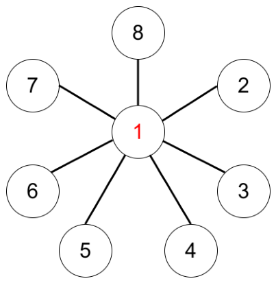
A star graph is a graph that contains a distinguished vertex, called the center, which is connected to all other vertices, while no edges exist between any pair of non-central vertices. This means that all objects are compared to the same distinguished one. Which object should be at the center to provide as much information as possible? If the directed graph corresponding to the data is strongly connected, then the data can be evaluated and the strengths can be estimated. If the directed graph generated by the dataset is not strongly connected, then there exists an object that is “better” or “worse” than the center, based on all decisions between it and the center. In this case, the likelihood function does not attain its maximum and the data cannot be evaluated. If this happens frequently, information retrieval becomes ineffective due to the impossibility of obtaining the required information applying maximum likelihood estimation and further techniques are required [47].

Figure 2 shows a star graph for n = 8 objects, with object 1 as the center. The center is compared with every other object.

Due to space limitations, only a few examples are presented herein for each case. For the star graph structure, first we present the results for parameter choices $n=8$, $d=0.25,0.5$, $l=25,50$. For the star graph, the results are shown in

Table 1. Results for star graph ($n=8,d=0.25,l=25$).

Center	D	CORR	$\mathit{\rho }$	$\mathit{\tau }$	Evaluable	IC
1	1.1937	0.8251	0.8302	0.7083	97.39%	0.0872
2	1.1295	0.8402	0.8441	0.7257	99.15%	0.0911
3	1.0833	0.8500	0.8547	0.7391	99.78%	0.0940
4	1.0554	0.8555	0.8617	0.7475	99.95%	0.0953
5	1.0564	0.8556	0.8615	0.7475	99.94%	0.0953
6	1.0823	0.8500	0.8544	0.7390	99.79%	0.0940
7	1.1308	0.8399	0.8435	0.7251	99.14%	0.0913
8	1.1935	0.8252	0.8300	0.7079	97.39%	0.0873
avg	1.1156	0.8427	0.8475	0.7300	99.07%	0.0919
complete	0.3970	0.9746	0.9783	0.9388	100.00%	0.0922

,

Table 2. Results for star graph ($n=8,d=0.25,l=50$).

Center	D	CORR	$\mathit{\rho }$	$\mathit{\tau }$	Evaluable	IC
1	0.8256	0.9018	0.9044	0.8041	99.96%	0.0620
2	0.7746	0.9119	0.9144	0.8210	100.00%	0.0647
3	0.7418	0.9182	0.9225	0.8327	100.00%	0.0665
4	0.7267	0.9211	0.9264	0.8374	100.00%	0.0676
5	0.7248	0.9216	0.9268	0.8382	100.00%	0.0674
6	0.7409	0.9185	0.9226	0.8330	100.00%	0.0665
7	0.7748	0.9118	0.9144	0.8210	100.00%	0.0647
8	0.8244	0.9021	0.9046	0.8045	99.96%	0.0619
avg	0.7667	0.9134	0.9170	0.8240	99.99%	0.0652
complete	0.2793	0.9871	0.9921	0.9765	100.00%	0.0652

,

Table 3. Results for star graph ($n=8,d=0.5,l=25$).

Center	D	CORR	$\mathit{\rho }$	$\mathit{\tau }$	Evaluable	IC
1	1.3655	0.9047	0.9026	0.8134	30.17%	0.0680
2	1.2657	0.9286	0.9319	0.8548	58.00%	0.0757
3	1.2428	0.9413	0.9490	0.8796	81.94%	0.0816
4	1.2321	0.9474	0.9569	0.8923	94.42%	0.0844
5	1.2343	0.9472	0.9568	0.8921	94.47%	0.0844
6	1.2412	0.9415	0.9493	0.8805	82.04%	0.0814
7	1.2664	0.9286	0.9317	0.8547	57.73%	0.0758
8	1.3626	0.9049	0.9031	0.8141	30.55%	0.0677
avg	1.2763	0.9305	0.9351	0.8602	66.16%	0.0774
complete	0.4827	0.9913	0.9969	0.9908	100.00%	0.0786

,

Table 4. Results for star graph ($n=8,d=0.5,l=50$).

Center	D	CORR	$\mathit{\rho }$	$\mathit{\tau }$	Evaluable	IC
1	1.1179	0.9457	0.9504	0.8868	69.13%	0.0482
2	1.0367	0.9587	0.9670	0.9172	89.52%	0.0540
3	0.9421	0.9674	0.9758	0.9348	97.91%	0.0582
4	0.8671	0.9723	0.9797	0.9434	99.83%	0.0601
5	0.8686	0.9721	0.9795	0.9430	99.81%	0.0602
6	0.9414	0.9674	0.9758	0.9351	97.82%	0.0581
7	1.0366	0.9586	0.9670	0.9177	89.12%	0.0542
8	1.1191	0.9457	0.9506	0.8867	69.56%	0.0482
avg	0.9912	0.9610	0.9682	0.9206	89.09%	0.0552
complete	0.3381	0.9956	0.9997	0.9991	100.00%	0.0556

,

Table 5. Results for different spanning trees ($n=8,d=0.25,l=25$).

Center	D	CORR	$\mathit{\rho }$	$\mathit{\tau }$	Evaluable	IC
avg spanning tree	1.2549	0.8097	0.8070	0.6811	99.04%	0.0919
avg star graph	1.1156	0.8427	0.8475	0.7300	99.07%	0.0919
opt. star graph	1.0554	0.8556	0.8617	0.7475	99.95%	0.0953

,

Table 6. Results for different spanning trees ($n=8,d=0.25,l=50$).

Center	D	CORR	$\mathit{\rho }$	$\mathit{\tau }$	Evaluable	IC
avg spanning tree	0.8649	0.8905	0.8891	0.7833	99.99%	0.0652
avg star graph	0.7667	0.9134	0.9170	0.8240	99.99%	0.0652
opt. star graph	0.7248	0.9216	0.9268	0.8382	100.00%	0.0674

,

Table 7. Results for different spanning trees ($n=8,d=0.5,l=25$).

Center	D	CORR	$\mathit{\rho }$	$\mathit{\tau }$	Evaluable	IC
avg spanning tree	1.4243	0.9163	0.9163	0.8254	64.00%	0.0787
avg star graph	1.2763	0.9305	0.9351	0.8602	66.16%	0.0774
opt. star graph	1.2321	0.9474	0.9569	0.8923	94.42%	0.0844

,

Table 8. Results for different spanning trees ($n=8,d=0.5,l=50$).

Center	D	CORR	$\mathit{\rho }$	$\mathit{\tau }$	Evaluable	IC
avg spanning tree	1.1141	0.9504	0.9533	0.8896	88.69%	0.0556
avg star graph	0.9912	0.9610	0.9682	0.9206	89.09%	0.0552
opt. star graph	0.8671	0.9723	0.9797	0.9434	99.83%	0.0601

and

Table 9. Results for different spanning trees applying Gaussian distribution ($n=8,d=0.25,l=25$).

Center	D	CORR	$\mathit{\rho }$	$\mathit{\tau }$	Evaluable	IC
avg spanning tree	1.2364	0.7826	0.7782	0.6494	99.51%	0.0935
avg star graph	1.0975	0.8188	0.8220	0.6998	99.49%	0.0934
opt. star graph	1.0489	0.8269	0.8304	0.7112	99.97%	0.0963
complete	0.4187	0.9692	0.9723	0.9241	100.00%	0.0935

in the case of the mentioned parameter settings. In the tables, the first column indicates which object is in the center of the star graph. Note that the object number refers to its serial number after sorting the objects in ascending order of their expected values. The last rows contain their averages, as well as the results obtained from evaluating the complete graph, respectively. The column Evaluable is the rate of cases that can be evaluated. The column IC is the average inconsistency index computed by taking the average of the values defined by (12). The optimal values are shown in bold in the tables.

Situations encountered in practice are often more complex than the previously considered scenarios. Therefore, we also investigate four further situations. In all cases, we use the parameters ($n=8$ and $l=50$), and generate the object strengths from a Gaussian distribution (denoted by $\mathcal{N}(\mu ,{\sigma }^2)$) with standard deviation 0.5.

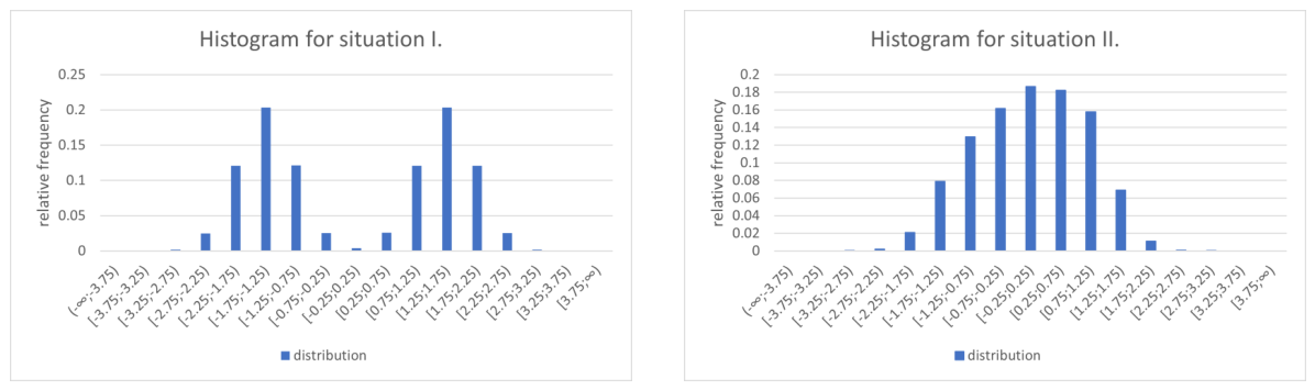
In situation I, the objects are divided into two groups; i.e., they can be classified into two clusters based on their strengths. For the first group, the strengths are generated as $m_i\sim \mathcal{N}(-1.5,0.5^2)$, whereas for the second group, $m_i\sim \mathcal{N}(1.5,0.5^2)$.

In situation II, the objects are divided into three groups; i.e.,; they form three clusters. The corresponding strengths are generated as $m_i\sim \mathcal{N}(-1,0.5^2)$, $m_i\sim \mathcal{N}(0,0.5^2)$, and $m_i\sim \mathcal{N}(1,0.5^2)$, respectively.

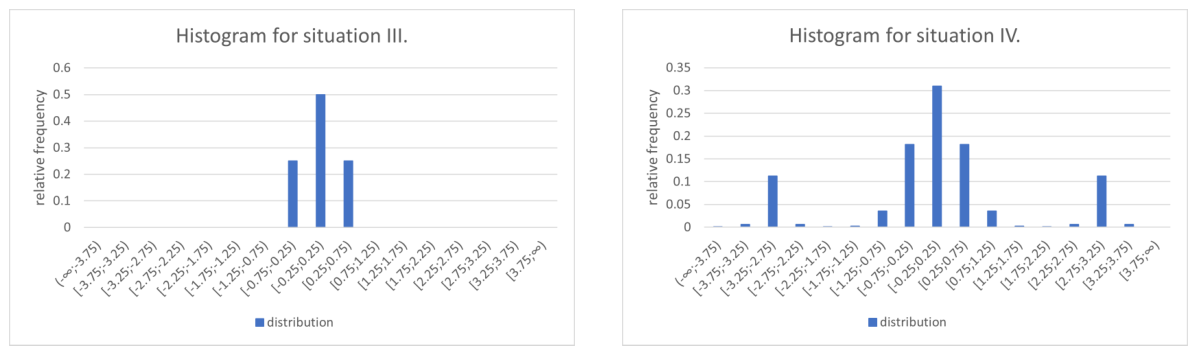
In situation III, the object strengths are fixed and differ only slightly, with a strength difference of $d=0.15$.

In Situation IV, there are fixed extreme objects and additional objects with randomly generated strengths. Two outliers with strengths $-3$ and 3 are introduced, while the strengths of the remaining objects are generated as $m_i\sim \mathcal{N}(0,0.5^2)$.

The corresponding histograms are shown in Figure 3 and Figure 4. The distributions of the generated original initial parameters are presented in

Table 10. Results for situation I ($n=8,l=50$).

Name	D	CORR	$\mathit{\rho }$	$\mathit{\tau }$	Evaluable	IC
1	1.1406	0.9636	0.9067	0.8098	33.87%	0.0456
2	1.1185	0.9679	0.9134	0.8195	51.83%	0.0478
3	1.1046	0.9709	0.9194	0.8274	66.71%	0.0490
4	1.0728	0.9744	0.9254	0.8346	81.41%	0.0500
5	1.0752	0.9743	0.9253	0.8375	81.51%	0.0500
6	1.1012	0.9710	0.9200	0.8322	66.70%	0.0489
7	1.1172	0.9679	0.9133	0.8218	51.56%	0.0476
8	1.1426	0.9635	0.9067	0.8080	33.93%	0.0455
avg	1.1091	0.9692	0.9163	0.8238	58.44%	0.0480
complete	0.3944	0.9971	0.9740	0.9317	100.00%	0.0496

,

Table 11. Results for situation II ($n=8,l=50$).

Name	D	CORR	$\mathit{\rho }$	$\mathit{\tau }$	Evaluable	IC
1	1.0232	0.9293	0.8987	0.8036	88.96%	0.0512
2	0.9142	0.9457	0.9175	0.8302	96.96%	0.0567
3	0.8326	0.9549	0.9294	0.8477	99.39%	0.0602
4	0.8058	0.9578	0.9331	0.8532	99.76%	0.0615
5	0.8056	0.9578	0.9336	0.8541	99.64%	0.0614
6	0.8453	0.9540	0.9296	0.8483	98.76%	0.0599
7	0.9045	0.9471	0.9216	0.8359	96.40%	0.0575
8	0.9891	0.9343	0.908	0.8142	90.02%	0.0532
avg	0.8900	0.9476	0.9215	0.8359	96.23%	0.0577
complete	0.3107	0.9933	0.9761	0.9372	100.00%	0.0594

,

Table 12. Results for situation III ($n=8,d=0.15,l=50$).

Name	D	CORR	$\mathit{\rho }$	$\mathit{\tau }$	Evaluable	IC
1	0.7322	0.8069	0.8036	0.6746	100.00%	0.0648
2	0.7156	0.8124	0.809	0.6833	100.00%	0.0659
3	0.7053	0.8172	0.8158	0.6935	100.00%	0.0667
4	0.7002	0.8181	0.8185	0.6977	100.00%	0.0671
5	0.6995	0.8183	0.8185	0.6978	100.00%	0.0671
6	0.7041	0.8170	0.8156	0.6936	100.00%	0.0666
7	0.7154	0.8127	0.8098	0.6844	100.00%	0.0659
8	0.7318	0.8073	0.8037	0.6743	100.00%	0.0648
avg	0.7130	0.8137	0.8118	0.6874	100.00%	0.0661
complete	0.2651	0.9677	0.9699	0.9184	100.00%	0.0679

and

Table 13. Results for situation IV ($n=8,l=50$).

Name	D	CORR	$\mathit{\rho }$	$\mathit{\tau }$	Evaluable	IC
1	2.7923	0.7791	0.6635	0.5768	0.66%	0.0423
2	1.3056	0.9573	0.876	0.7823	41.46%	0.0781
3	1.1972	0.9646	0.8804	0.7895	46.45%	0.0806
4	1.1584	0.9669	0.8817	0.7928	48.01%	0.0812
5	1.1551	0.9672	0.8817	0.7930	48.20%	0.0810
6	1.1949	0.9648	0.8807	0.7902	46.30%	0.0802
7	1.3069	0.9572	0.8764	0.7826	41.09%	0.0782
8	2.7796	0.7833	0.6781	0.5898	0.67%	0.0417
avg	1.6112	0.9175	0.8273	0.7371	0.3410338	0.0704
complete	0.6247	0.9935	0.9529	0.8935	99.84%	0.0743

.

4.2. Union of Two Star Graphs Structure

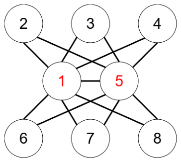
The next structure to be investigated is the union of two star graphs. This structure is investigated in-depth in multi-criteria decision-making [19,26]. The union of two star graphs is shown in Figure 5. In the example shown, objects 1 and 5 are compared to all the other objects, as well as to each other. If we consider another union of two star graphs, the structure is isomorphic to the structure that can be seen in Figure 5. In previous publications, cases were investigated in which the best and worst objects, the best and second–best objects, or the best object and a randomly selected object were jointly placed at the centers of the union of two star graphs [19,26].

Investigating the union of two star graphs structure, for the parameter choices $n=8$, $d=0.25,0.5$, $l=25,50$, the results are shown in

Table 14. Results for the union of two star graphs ($n=8,d=0.25,l=25$).

Centers	D	CORR	$\mathit{\rho }$	$\mathit{\tau }$	Evaluable	IC
(1,2)	0.7681	0.9129	0.9157	0.8221	99.99%	0.0887
(1,3)	0.7436	0.9179	0.9202	0.8275	100.00%	0.0903
(1,4)	0.7280	0.9211	0.9232	0.8313	100.00%	0.0914
(1,5)	0.7182	0.9227	0.9242	0.8325	100.00%	0.0918
(1,6)	0.7140	0.9231	0.9225	0.8306	100.00%	0.0914
(1,7)	0.7193	0.9214	0.9178	0.8232	100.00%	0.0904
(1,8)	0.7293	0.9185	0.9141	0.8157	100.00%	0.0887
(2,3)	0.7248	0.9220	0.9260	0.8388	100.00%	0.0922
(2,4)	0.7124	0.9246	0.9274	0.8388	100.00%	0.0932
(2,5)	0.7043	0.9261	0.9272	0.8390	100.00%	0.0935
(2,6)	0.7028	0.9260	0.9251	0.8367	100.00%	0.0931
(2,7)	0.7078	0.9245	0.9215	0.8311	100.00%	0.0920
(2,8)	0.7177	0.9217	0.9178	0.8233	100.00%	0.0905
(3,4)	0.7000	0.9276	0.9340	0.8498	100.00%	0.0944
(3,5)	0.6948	0.9284	0.9321	0.8459	100.00%	0.0946
(3,6)	0.6967	0.9277	0.9289	0.8426	100.00%	0.0941
(3,7)	0.7024	0.9263	0.9255	0.8374	100.00%	0.0931
(3,8)	0.7138	0.9232	0.9224	0.8305	100.00%	0.0915
(4,5)	0.6910	0.9294	0.9368	0.8533	100.00%	0.0951
(4,6)	0.6954	0.9284	0.9323	0.8462	100.00%	0.0946
(4,7)	0.7051	0.9261	0.9273	0.8394	100.00%	0.0935
(4,8)	0.7171	0.9229	0.9244	0.8327	100.00%	0.0918
(5,6)	0.6995	0.9274	0.9337	0.8494	100.00%	0.0945
(5,7)	0.7116	0.9247	0.9274	0.8390	100.00%	0.0932
(5,8)	0.7278	0.9209	0.9230	0.8309	100.00%	0.0915
(6,7)	0.7273	0.9215	0.9255	0.8382	100.00%	0.0923
(6,8)	0.7465	0.9173	0.9195	0.8263	100.00%	0.0905
(7,8)	0.7693	0.9128	0.9152	0.8213	99.99%	0.0888
avg	0.7175	0.9231	0.9247	0.8348	100.00%	0.0922
complete	0.3972	0.9745	0.9782	0.9387	100.00%	0.0922

,

Table 15. Results for the union of two star graphs ($n=8,d=0.25,l=50$).

Centers	D	CORR	$\mathit{\rho }$	$\mathit{\tau }$	Evaluable	IC
(1,2)	0.5314	0.9537	0.9565	0.8932	100.00%	0.0628
(1,3)	0.5160	0.9566	0.9590	0.8969	100.00%	0.0639
(1,4)	0.5055	0.9585	0.9611	0.9003	100.00%	0.0647
(1,5)	0.4995	0.9596	0.9620	0.9016	100.00%	0.0649
(1,6)	0.4983	0.9596	0.9614	0.9008	100.00%	0.0647
(1,7)	0.5009	0.9589	0.9589	0.8968	100.00%	0.0639
(1,8)	0.5092	0.9568	0.9556	0.8884	100.00%	0.0628
(2,3)	0.5033	0.9592	0.9634	0.9070	100.00%	0.0652
(2,4)	0.4951	0.9608	0.9635	0.9070	100.00%	0.0659
(2,5)	0.4903	0.9616	0.9646	0.9087	100.00%	0.0661
(2,6)	0.4910	0.9614	0.9641	0.9078	100.00%	0.0659
(2,7)	0.4938	0.9606	0.9618	0.9041	100.00%	0.0651
(2,8)	0.5022	0.9586	0.9586	0.8962	100.00%	0.0640
(3,4)	0.4872	0.9624	0.9674	0.9137	100.00%	0.0667
(3,5)	0.4841	0.9629	0.9664	0.9118	100.00%	0.0668
(3,6)	0.4849	0.9627	0.9666	0.9123	100.00%	0.0665
(3,7)	0.4900	0.9616	0.9643	0.9082	100.00%	0.0658
(3,8)	0.4980	0.9598	0.9616	0.9012	100.00%	0.0647
(4,5)	0.4819	0.9634	0.9685	0.9155	100.00%	0.0672
(4,6)	0.4846	0.9628	0.9665	0.9119	100.00%	0.0669
(4,7)	0.4900	0.9617	0.9648	0.9091	100.00%	0.0660
(4,8)	0.5002	0.9596	0.9621	0.9019	100.00%	0.0649
(5,6)	0.4872	0.9623	0.9674	0.9137	100.00%	0.0668
(5,7)	0.4958	0.9606	0.9634	0.9066	100.00%	0.0659
(5,8)	0.5063	0.9585	0.9611	0.9003	100.00%	0.0647
(6,7)	0.5034	0.9591	0.9633	0.9066	100.00%	0.0653
(6,8)	0.5163	0.9565	0.9588	0.8966	100.00%	0.0640
(7,8)	0.5315	0.9537	0.9567	0.8933	100.00%	0.0628
avg	0.4992	0.9598	0.9625	0.9040	100.00%	0.0652
complete	0.2794	0.9871	0.9921	0.9765	100.00%	0.0652

,

Table 16. Results for the union of two star graphs ($n=8,d=0.5,l=25$).

Centers	D	CORR	$\mathit{\rho }$	$\mathit{\tau }$	Evaluable	IC
(1,2)	1.0627	0.9543	0.9613	0.9066	81.93%	0.0707
(1,3)	1.0131	0.9612	0.9687	0.9208	92.02%	0.0748
(1,4)	0.9536	0.9668	0.9742	0.9312	97.79%	0.0773
(1,5)	0.8964	0.9708	0.9769	0.9364	99.69%	0.0783
(1,6)	0.8746	0.9721	0.9768	0.9359	99.99%	0.0774
(1,7)	0.8938	0.9707	0.9738	0.9302	100.00%	0.0749
(1,8)	0.9501	0.9668	0.9680	0.9162	100.00%	0.0708
(2,3)	0.9692	0.9652	0.9738	0.9317	95.24%	0.0782
(2,4)	0.9120	0.9698	0.9778	0.9405	98.70%	0.0804
(2,5)	0.8628	0.9731	0.9801	0.9451	99.82%	0.0814
(2,6)	0.8405	0.9744	0.9804	0.9455	100.00%	0.0807
(2,7)	0.8524	0.9736	0.9782	0.9413	100.00%	0.0785
(2,8)	0.8937	0.9707	0.9738	0.9303	100.00%	0.0748
(3,4)	0.8732	0.9723	0.9802	0.9449	99.42%	0.0827
(3,5)	0.8393	0.9745	0.9817	0.9484	99.92%	0.0834
(3,6)	0.8275	0.9753	0.9823	0.9495	99.99%	0.0828
(3,7)	0.8408	0.9744	0.9805	0.9459	99.98%	0.0808
(3,8)	0.8754	0.9720	0.9768	0.9360	99.97%	0.0774
(4,5)	0.8305	0.9750	0.9821	0.9490	99.94%	0.0840
(4,6)	0.8389	0.9746	0.9817	0.9485	99.91%	0.0833
(4,7)	0.8623	0.9731	0.9802	0.9453	99.80%	0.0813
(4,8)	0.8973	0.9708	0.9769	0.9365	99.69%	0.0782
(5,6)	0.8728	0.9724	0.9801	0.9448	99.41%	0.0826
(5,7)	0.9111	0.9698	0.9776	0.9401	98.70%	0.0804
(5,8)	0.9523	0.9669	0.9742	0.9312	97.86%	0.0772
(6,7)	0.9694	0.9652	0.9739	0.9321	95.28%	0.0781
(6,8)	1.0151	0.9612	0.9688	0.9210	92.21%	0.0746
(7,8)	1.0648	0.9542	0.9609	0.9061	81.80%	0.0707
avg	0.9088	0.9693	0.9758	0.9354	97.47	0.0784
complete	0.4827	0.9913	0.9969	0.9908	100.00%	0.0786

and

Table 17. Results for the union of two star graphs ($n=8,d=0.5,l=50$).

Centers	D	CORR	$\mathit{\rho }$	$\mathit{\tau }$	Evaluable	IC
(1,2)	0.8240	0.9740	0.9818	0.9506	97.84%	0.0500
(1,3)	0.7397	0.9790	0.9862	0.9614	99.55%	0.0529
(1,4)	0.6645	0.9829	0.9891	0.9685	99.96%	0.0547
(1,5)	0.6156	0.9853	0.9907	0.9728	100.00%	0.0553
(1,6)	0.6032	0.9859	0.9911	0.9736	100.00%	0.0547
(1,7)	0.6171	0.9852	0.9900	0.9709	100.00%	0.0529
(1,8)	0.6545	0.9831	0.9866	0.9614	100.00%	0.0500
(2,3)	0.6895	0.9816	0.9885	0.9672	99.82%	0.0553
(2,4)	0.6302	0.9846	0.9912	0.9744	99.98%	0.0569
(2,5)	0.5913	0.9865	0.9927	0.9785	100.00%	0.0575
(2,6)	0.5796	0.9871	0.9932	0.9798	100.00%	0.0571
(2,7)	0.5898	0.9866	0.9925	0.9782	100.00%	0.0555
(2,8)	0.6187	0.9851	0.9899	0.9705	100.00%	0.0529
(3,4)	0.6001	0.9860	0.9918	0.9758	99.99%	0.0585
(3,5)	0.5742	0.9873	0.9933	0.9801	100.00%	0.0589
(3,6)	0.5704	0.9876	0.9936	0.9808	100.00%	0.0586
(3,7)	0.5807	0.9871	0.9932	0.9797	100.00%	0.0572
(3,8)	0.6042	0.9859	0.9910	0.9734	100.00%	0.0548
(4,5)	0.5684	0.9875	0.9929	0.9789	100.00%	0.0594
(4,6)	0.5753	0.9872	0.9932	0.9798	100.00%	0.0590
(4,7)	0.5921	0.9865	0.9926	0.9783	100.00%	0.0576
(4,8)	0.6178	0.9852	0.9906	0.9725	100.00%	0.0554
(5,6)	0.5977	0.9861	0.9919	0.9762	99.99%	0.0584
(5,7)	0.6288	0.9846	0.9912	0.9744	99.99%	0.0569
(5,8)	0.6627	0.9829	0.9891	0.9687	99.96%	0.0547
(6,7)	0.6889	0.9816	0.9886	0.9675	99.84%	0.0553
(6,8)	0.7396	0.9789	0.9862	0.9614	99.57%	0.0529
(7,8)	0.8257	0.9739	0.9817	0.9504	97.78%	0.0500
avg	0.6373	0.9841	0.9901	0.9716	99.80%	0.0555
complete	0.3374	0.9956	0.9997	0.9991	100.00%	0.0555

. The first column shows which object-pair is placed at the two central points of the union of the two star graphs. Meanwhile, the last rows contain the averages and the results computed using the entire dataset for the purpose of a comprehensive comparison.

4.3. Union of Two Edge-Disjoint Spanning Trees

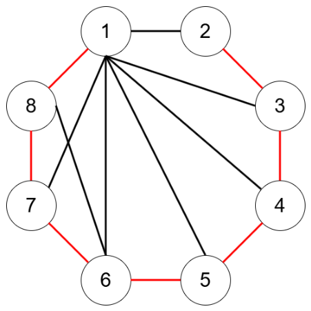
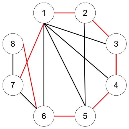
In [19], the authors investigated the PCM-based model with LLSM and CREV evaluation methods, and found that, on average, the union of two edge-disjoint spanning trees is a better comparison structure, than the union of two star graphs structure. In this case the number of compared pairs equals $2·(n-1)$, and in the case of the union of two star graphs, this number equals $2·(n-1)-1=2·n-3$. A union of two star graphs is the union of two spanning trees, however, these are not edge-disjoint, since they must have a common edge. According to the findings [15,20] a larger number of comparison pairs leads to better information retrieval, in average, but only in the case of optimal comparison structures. Two unions of two star graphs are always isomorphic to each other. However, the union of two star graphs does not belong to the class of optimal structures, since the degrees of the vertices differ significantly: the central vertices have a degree of $n-1$, while the non central vertices have a degree of only 2.

Nevertheless, the union of two edge-disjoint spanning trees may result in different comparison graph structures. Such examples are presented in Figure 6 and Figure 7. The resulting two comparison graphs are not isomorphic: in example in Figure 6, there is one vertex of degree 7, while in the example in Figure 7, the maximum number of edges from a vertex is 6. (The two spanning trees are shown in different colors in the figures.)

During the simulations, we randomly generated a union of two edge-disjoint spanning trees as follows. Using a uniformly distributed random number generator, we selected edges one after the other in such a way as to obtain a spanning tree. If the selected edge would form a circle, we discarded this edge. If the graph has $n-1$ edges and it does not contain any cycle, it must be a spanning tree. Once we obtained the first spanning tree, we generated the second spanning tree in the same way, but in this case we excluded the edges that were already contained in the first spanning tree. The union of the two spanning trees obtained in this way will be a union of two edge-disjoint spanning trees.

The results for the union of two edge-disjoint spanning trees are detailed in

Table 18. Results for the star graph structure, union of two edge-disjoint spanning trees and the union of the two star graphs ($n=8,d=0.25,l=25$).

Name	D	CORR	$\mathit{\rho }$	$\mathit{\tau }$	Evaluable	IC
avg star graph (l = 50)	0.7667	0.9134	0.9170	0.8240	99.99%	0.0652
avg u. of two star graphs	0.7175	0.9231	0.9247	0.8348	100.00%	0.0922
avg u. of two edge-disjoint sp. trees	0.6586	0.9340	0.9330	0.8461	100.00%	0.0922

,

Table 19. Results for the star graph structure, union of two edge-disjoint spanning trees and the union of two star graphs ($n=8,d=0.25,l=50$).

Name	D	CORR	$\mathit{\rho }$	$\mathit{\tau }$	Evaluable	IC
avg star graph (l = 100)	0.5323	0.9545	0.9578	0.8946	100.00%	0.0461
avg u. of two star graphs	0.4992	0.9598	0.9625	0.9040	100.00%	0.0652
avg u. of two edge-disjoint sp. trees	0.4593	0.9656	0.9675	0.9141	100.00%	0.0652

,

Table 20. Results for the star graph structure, union of two edge-disjoint spanning trees and union of the two star graphs ($n=8,d=0.5,l=25$).

Name	D	CORR	$\mathit{\rho }$	$\mathit{\tau }$	Evaluable	IC
avg star graph (l = 50)	0.9912	0.9610	0.9682	0.9206	89.09%	0.0556
avg u. of two star graphs	0.9088	0.9693	0.9758	0.9354	97.47%	0.0785
avg u. of two edge-disjoint sp. trees	0.8343	0.9744	0.9789	0.9420	99.00%	0.0786

and

Table 21. Results for the star graph structure, union of two edge-disjoint spanning trees and the union of two star graphs ($n=8,d=0.5,l=50$).

Name	D	CORR	$\mathit{\rho }$	$\mathit{\tau }$	Evaluable	IC
avg star graph (l = 100)	0.7326	0.9787	0.9857	0.9606	98.32%	0.0392
avg u. of two star graphs	0.6373	0.9841	0.9901	0.9716	99.80%	0.0555
avg u. of two edge-disjoint sp. trees	0.5792	0.9868	0.9920	0.9766	99.93%	0.0556

. The third row shows the average values for the union of two edge-disjoint spanning trees; the second row shows the average values obtained for the union of two star graphs, while the first row shows the average values for the star graph structure with twice as many comparisons by each pair.

5. Discussion

5.1. General Observations

First, note that for D metrics, a lower value is better, while for the correlations, a higher value expresses better information retrieval. All four similarity metrics—D, CORR, $\rho$, and $\tau$—demonstrably exhibit the same phenomenon: in general, a lower D value results in larger CORR, $\rho$, and $\tau$ values. This also implies that generally all of the four metrics select the same placement (object or object pair) as the optimal one. Consequently, the universally optimal placement exists in most cases. If, on rare occasions, this is not the case, see for example Table 1, there are marginal differences between the values, which may be attributed to simulation error. Otherwise, in Table 1, three similarity measures yield the same optimal placement, that is, they place object 4 at the center. Although the universally optimal placement does not exist in this case, one of the two middle position objects, i.e., 4 or 5 are assigned as optimal according to each similarity measure. Nevertheless, choosing object 4 or 5, only minor changes can be found in the similarity metrics.

As expected, if more comparisons are made between the objects (i.e., l is higher), better values are obtained for a given parameter setting. This can be explained by the fact that in the case of consistent data, the incomplete dataset contains all of the information. The last rows of the tables also indicate that the metrics computed from the complete comparison data are much more better than the metrics computed based on the incomplete comparisons. This remains valid even for average values and for the case of optimal placement. This is in line with the fact that, for the same number of observers, more comparisons lead to greater information retrieval. The total number of compared pairs is $n·(n-1)/2$, which is larger than $2·(n-1)$ and also $2·n-3$. However, if the product of the numbers of compared pairs and the number of observers (l) is approximately the same, that also yields approximately the same values for the metrics. If we compare the metrics of the star graphs and $l=50$, we can see similar average D, CORR, $\rho$ and $\tau$ values than in the case of the union of two star graphs for $l=25$ even in the case $d=0.25$ and $d=0.5$. If $l=50$ instead of $l=25$, it means that the number comparisons on each pair has increased, but the entire numbers of comparisons are close to each other.

Regarding the IC values, they are definitely less in case of star graph structure for $l=50$, than for the union of two star graphs for $l=25$. Larger datasets exhibit greater consistency: the relative frequency better approximates the probability in simulations. This phenomenon is observable via the definite decrease of the IC metrics, when comparing the IC metrics for $l=25$ and $l=50$ under the same d parameter.

5.2. Discussion of Star Graph Structure’s Results

In the case of star graph structure, n different objects can be placed into the center. There are always $n-1$ compared pairs. Fixing the parameter d, Table 1 and Table 2, as well as Table 3 and Table 4 show that for each object, the information retrieval is better with a larger number of comparisons by compared pairs ($l=50$) than with a lower number of comparisons by compared pairs ($l=25$). This is also the case for the rate of evaluable simulations. When comparing Table 1 and Table 3, as well as Table 2 and Table 4, the D and correlation measures are observably higher for larger differences in the parameters, while the number of evaluable cases decreases as the distance between the expectations increases. This can be explained by the fact that bidirectional relations between the center and the other objects are required, which occur less frequently when the distance between them is significant.

If the value of the observer (l) is fixed, the smaller d parameter value demonstrably results in a larger number of evaluable cases, and the difference is large.

As the other tables also indicate, if the value of d is larger, fewer cases can be evaluated, this yields worse results in the various rank correlation indices, while in the case of D, this yields worse results. The best-case scenario is always when all comparisons are available—that is, when we have a complete graph—but this is self-evident, given that the complete graph significantly outperforms star graphs in terms of the number of comparisons.

Upon considering the values of the inconsistency metric, an increase in the number of comparisons by pairs results in improvement. If we compare them in fixed parameter settings, they are the smallest when the extreme strength objects are placed into the center. This observation is similar the observation in [26].

The four tables show similarities in the individual metrics when applied to the different placements. On the one hand, the results are symmetric with respect to the object of intermediate strength, with only small deviations; these may arise from the random nature of the simulations. On the other hand, one of the intermediate objects always performs best. Although in some cases its advantage over the other placements is only minor in terms of metrics (see Table 1 and Table 2), where there are enormous differences in terms of evaluability, especially when the number of comparisons (l) is small and the strength difference (d) is large (see Table 3 and Table 4). Even in the absence of other advantages, this placement is still highly preferable because the data obtained from it can be evaluated with significantly greater certainty.

In order to observe the advantage of the optimal placement in the star graph structure, we compared the average performances of spanning trees, the average performances of star graphs and the performance of the optimal star graph in Table 5, Table 6, Table 7 and Table 8. The results indicate that the star graph with the optimal placement outperforms the average spanning trees by about 15% in terms of the D metric, and the average star graph structure by about 10%. Considerable improvements are also observable in the correlations. The IC metric exhibits the opposite behavior, with the average of star graph comparison structure exhibiting the lowest values.

The cases in Situations I–IV differ substantially from both the previous cases and from one another in terms of their initial (original) data, as clearly illustrated by their corresponding histograms. Nevertheless, the same phenomena observed in the previous (controlled and uniformly distributed) cases can be seen, although the differences are less pronounced in some instances (see Table 10, Table 11, Table 12 and Table 13).

5.3. Discussion of the Union of Two Star Graphs Structure’s Results

For the union of two star graphs structure, the placement of specific objects in the centers is not as certain as it is with star graphs.

For the same number of decisions by pairs, the number of comparisons increases by approximately a factor of two. The symmetry of the metrics around the index value (4,5) can be observed: D, CORR, $\rho$, $\tau$, and IC values are very similar for (1,2) and (7,8), as well as (3,5) and (4,6) pairs. It remains true that placing objects of intermediate strength at the center is beneficial. Regarding D, CORR, $\rho$ and $\tau$, when the centers of the union of two star graphs are chosen from the middle third strength elements, the metrics are very close to each other for fixed parameter values.

Previous studies have often recommended or focused exclusively on best case/worst case comparisons. Comparisons with intermediate objects have not been common. From Table 14, Table 15, Table 16 and Table 17 it is clear that neither best-worst (1,8), nor TOP2 (7,8) in the centers can be recommended. They are even worse than the average in each presented cases, for all metrics. The placement (4,5) proves to be the optimal in the cases presented in Table 14, Table 15 and Table 16, while in Table 17 the pair (4,5) performs optimal in terms of D and the pair (3,6) in terms of correlations. Only very small differences can be observed between the respective metrics for these pairs; 0.002 is within D values and under 0.001 within the correlations. These are under the error of the simulations. Nevertheless, there are significant differences between the metrics corresponding to these pairs and those corresponding to the pairs (1,8) or (7,8); the D values differ by more than 0.25, and the differences in the correlations over than ten times larger than in the previous case. The performances of the optimal placements outperform the average (avg) by 10% in terms of the D metric, and there are significant improvements in correlations as well.

Concerning the evaluability, almost all cases are evaluable, except for the parameters $n=8,d=0.5,l=25$. In this case, neither best-worst nor TOP2 placement is preferable: they produce the worst evaluable rates (81.93% and 81.80%). However, from the perspective of consistency, the pairs (1,8), (1,2) and (7,8) are the best. This observation is consistent with finding in [26], that the best-worst placement yields the lowest data inconsistency, with the additional note that the TOP2 arrangement is similarly favorable in terms of consistency.

5.4. Discussion of the Union of Two Edge-Disjoint Spanning Trees Structure’s Results

Finally, we compared the union of two star graphs structure’s results with the results given by the union of two edge-disjoint spanning trees, as it was investigated in [19]. Since the union of two edge-disjoint spanning trees does not correspond to a unique comparison graph structure, moreover, there is a substantial number of such comparisons, which result in of non-isomorphic graphs, we took the averages in the case of different metrics. The results for different parameter selection are observable in Table 18, Table 19, Table 20 and Table 21 for the Bradly-Terry model and in

Table 22. Results for the star graph structure, union of two edge-disjoint spanning trees and the union two star graphs applying Gaussian distribution ($n=8,d=0.25,l=25$).

Name	D	CORR	$\mathit{\rho }$	$\mathit{\tau }$	Evaluable	IC
avg star graph (l = 50)	0.7610	0.8988	0.9015	0.8004	100.00%	0.0661
avg u. of two star graphs	0.7173	0.9089	0.9094	0.8107	100.00%	0.0936
avg u. of two edge-disjoint sp. trees	0.6606	0.9216	0.9197	0.8239	100.00%	0.0936

if we use Gaussian distribution.

When comparing the average results in Table 18, Table 19, Table 20 and Table 21, obtained under different parameter settings, the union of two edge-disjoint spanning trees observably exhibits the same phenomenon as the star graph: all four metrics show the same behavior. Increasing the number of comparisons by pairs improves the information retrieval metrics, larger d values increase the D value and also the correlations, but reduce the number of evaluable cases.

Table 18 and Table 22 indicate that the performance metrics are sporadically better or worse for the Gaussian distribution than for the logistic distribution. For ease of comparison, the tables include the average values for the star graphs with twice as many comparisons, as well as the average metric values for the union of two star graphs. The observable conclusion is that the union of two edge-disjoint spanning trees performs best, in average, by D, and the correlations; the union of two star graphs structure comes next, followed by the star graph, which is the last of the three options, in average. Nevertheless, from the perspective of IC, the average star graph is definitely preferable to the others.

Finally, we compared the average metrics corresponding to the different structures and the metrics corresponding to the optimal placement in the cases of star graph and the union of two star graphs structure. The results are summarized in

Table 23. Results for fixed expectation values ($n=8,d=0.5,l=52,28,26$).

Name	D	CORR	$\mathit{\rho }$	$\mathit{\tau }$	Evaluable	IC
avg star graph (l = 52)	0.9759	0.9622	0.9695	0.9233	89.92%	0.0539
opt. star graph (l = 52)	0.8485	0.9733	0.9806	0.9455	99.87%	0.0592
avg of union of two star graphs (l = 28)	0.8593	0.9723	0.9788	0.9425	98.19%	0.0742
opt. union of two star graphs (l = 28)	0.7767	0.9779	0.9847	0.9557	100.00%	0.0781
avg u. of two edge-disjoint sp. trees (l = 26)	0.8161	0.9753	0.9799	0.9445	99.19%	0.0768

,

Table 24. Results for uniformly distributed $\underline{m}$ parameters ($n=8,d=0.5,l=52,28,26$).

Name	D	CORR	$\mathit{\rho }$	$\mathit{\tau }$	Evaluable	IC
avg star graph (l = 52)	0.8925	0.9504	0.9175	0.8299	96.30%	0.0583
opt. star graph (l = 52)	0.8038	0.9602	0.9294	0.8467	99.56%	0.0616
avg of union of two star graphs (l = 28)	0.7839	0.9618	0.9277	0.8445	99.28%	0.0794
opt. union of two star graphs (l = 28)	0.7371	0.9667	0.9368	0.8583	99.85%	0.0837
avg u. of two edge-disjoint spanning trees (l = 26)	0.7446	0.9655	0.9291	0.8450	99.65%	0.0825

and

Table 25. Results for standard Gaussian distributed $\underline{m}$ parameters ($n=8,d=0.5,l=52,28,26$).

Name	D	CORR	$\mathit{\rho }$	$\mathit{\tau }$	Evaluable	IC
avg star graph (l = 52)	0.8661	0.9451	0.9115	0.8248	94.08%	0.0592
opt. star graph (l = 52)	0.7928	0.9554	0.9249	0.8442	98.94%	0.0624
avg of union of two star graphs (l = 28)	0.7747	0.9577	0.9234	0.8413	98.56%	0.0806
opt. union of two star graphs (l = 28)	0.7325	0.9628	0.9336	0.8572	99.29%	0.0849
avg u. of two edge-disjoint sp. trees (l = 26)	0.7393	0.9615	0.9255	0.8425	99.19%	0.0837

. We ensured that the total numbers of comparisons were equal (364), so in the case of star graphs, the union of two star graphs and the union of two edge-disjoint spanning trees we made 52, 28, and 26 comparisons for each pair, respectively. This means that if the cost of a comparison is fixed, all data collection requires the same amount of resources. The simulations were performed for fixed and randomly generated expectations both for uniform and Gaussian distribution.

From Table 23, Table 24 and Table 25 it is observable that the optimal placement in the case of the union of two star graphs outperforms the average values corresponding to the two edge-disjoint spanning trees according to all four metrics and also by the percentage of evaluable datasets. This is confirmed independently of the distributions of the parameters. Therefore, for a fixed cost, when preliminary information about the ranking is available, it is rather worth applying the union of two star graphs structure with intermediate strength objects in the centers than the star graph structure, and than the union of two edge-disjoint spanning trees with randomly chosen spanning trees. Presumably, the optimal placement for the union of edge-disjoint spanning trees is better; however, our research does not analyze such placements systematically, as the number of possible placements is prohibitively large.

5.5. Similarity and Differences Between the Results in PCM-Based and THMM Models

In this subsection, we compare the findings concerning the placement of objects in PCM-based and THMM models. Since the previous results concern the PCM-based models, we can compare our observations with those reported by Szádoczki et al. [19], as well as by Rezaei [17]. In both cases, for PCMs and THMMs alike, only simulation-based results are available due to the of the complexity of the evaluation methods. Nevertheless, these observations can be useful for experiment design.

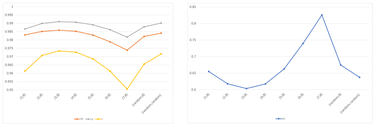
Overall, the results of the two model types exhibit a high degree of agreement across the cases examined, both in terms of D and correlations. This is also advantageous because it eliminates the need to decide before data collection which method will be used for the evaluation. While in the case of PCMs Szádoczki et al. [19] compared the frequently applied best-worst centered union of two star graphs structure to TOP2 centered union of two star graphs structure, we have placed each pair in the center of the graphs systematically. To illustrate, the results are presented for the parameter choices $d=0.5$ and $l=50$ in Figure 8. The best object is object 8, which is paired with object $1,\cdots ,7$. The correlations are plotted on the left, the D values are plotted on the right. “(random,8)” corresponds to the random-best choice, while the values plotted at “(random,random)” were computed when both centers were chosen randomly. The largest observable correlations belong to (3,8) and at the same time this placement has the smallest value of D. Therefore, when comparisons to the best are required, the optimal placement is (3,8) by all four metrics. Moreover, the correlations corresponding to the best-worst placement are lower than those corresponding to “(random,best)” placement. Upon the investigation of D metrics, the (3,8) placement has the lowest value. Although the best-worst placement yields a lower distance than the “(random,best)” placement, “(random,random)” placement is better.

For PCMs, however, the best-worst placement was found to be suboptimal, and our experiments also confirmed this for the THMM case. In the case of PCMs, the TOP2 placement proved to be preferable when compared to best-worst placement, however, this generally does not apply to THMMs. The best-worst placement corresponds to (1,8), while the TOP2 placement corresponds to (7,8). The metrics corresponding to this placement are worse than those corresponding to best-worst placement in the presented case. Szádoczki et al. show that best-random placement is better than best-worst placement. This also extends to THMMs in case of the correlations, but not in the case of D metrics. The observation that the “(random,random)” placement outperforms best-worst placement is consistent with the observation in [19] according to all four metrics. Szádoczki et al. report that on average, the union of two edge-disjoint spanning trees provides better information retrieval performance, than the best-random placement. The results indicate this also extends to THMMs.

Rezaei [26] argues for best-worst placement in the case of the union of two star graphs because it provides the best rate of evaluable datasets. This is not the case if we use THMM models. The reason is the stricter condition of evaluability: instead of connectivity of the graph of comparisons the strong connectivity is required. This is the consequence of the fact that in PCM-based models, the decisions are converted into numbers, whereas decisions are relations in THMMs, which means less information.

Concerning the data inconsistency, Rezaei et al. report smaller inconsistency values in the case of best-worst placement. This observation is consistent with ours, which indicates that best-worst placement yields more consistent data than alternative arrangements. This is also consistent with the intuition: the preferences can be determined with the least uncertainty relative to the strongest and the weakest objects.

The similarity of the findings for PCMs and THMMs strengthens the conjecture that different types of models may share a common underlying root that has not yet been identified.

6. Conclusions

The significance of the results lies in the fact that carefully planning the placement of objects in comparisons and incorporating prior information allows more information to be extracted from the resulting data than would be possible with random placement.

The paper investigates whether, for certain comparison structures, information retrieval can be improved by exploiting prior information about the ranking. The answer is affirmative: for star graph and the union of two star graphs structures, selecting medium-strength objects at the centers of the graphs can lead to a significant improvement compared to the worst or even the average values. Based on detailed investigations, it has been presented that the usually applied best case/worst case scenario and also the TOP2 placement is worse than those placements when objects from the middle third strengths are in the centers of the union of the two star graphs. However, this strongly contradicts previous practice [48,49,50]. The findings suggest that objects should be compared not to those at the extremes but to those of intermediate strength.

This raises the question of whether we can determine which objects have intermediate strength. Simulations demonstrate that there are few differences between the metrics when the objects are in the middle third, but there is a substantial improvement compared to extreme-strength objects. Once the extreme-strength objects are identified, they can be excluded as potential centers of a star graph. Moreover, consistent with previous research, our findings indicate that the union of two edge-disjoint spanning trees provides additional information compared to the union of two star graphs in terms of information retrieval.

No such detailed and systematic research has been conducted in this field before. These are the first results in this area with regard to stochastic models. Moreover, it would be worthwhile to conduct the same detailed investigations for PCM-based models. Could these properties be inherent to the models?

Our future work will focus on extending the research to additional comparison structures in order to investigate which arrangements enable more accurate parameter estimation.

It would represent a major breakthrough in understanding these models if it could be mathematically proven why it is worthwhile to compare other objects to an intermediate object. Understanding the reasons why these configurations perform well can lead to a deeper understanding of the Thurstone-motivated models, which in turn can enable better utilization of their potential in both forecasting and information retrieval.

References

1. Zhu, C. Artificial Intelligence Applications in Everyday Life. Appl. Comput. Eng. 2025, 121, 191–197. [Google Scholar] [CrossRef] [Scilit]
2. Xu, P.; Ji, X.; Li, M.; Lu, W. Small data machine learning in materials science. Comput. Mater. 2023, 9, 42. [Google Scholar] [CrossRef] [Scilit]
3. Rather, I.H.; Kumar, S.; Gandomi, A.H. Breaking the data barrier: A review of deep learning techniques for democratizing AI with small datasets. Artif. Intell. Rev. 2024, 57, 226. [Google Scholar] [CrossRef] [Scilit]
4. Gyarmati, L.; Orbán-Mihálykó, É.; Mihálykó, C.; Vathy-Fogarassy, Á. Aggregated Rankings of Top Leagues’ Football Teams: Application and Comparison of Different Ranking Methods. Appl. Sci. 2023, 13, 4556. [Google Scholar] [CrossRef] [Scilit]
5. Naser, M.Z. A review of machine learning with small and limited data. J. Big Data 2026, 13, 18. [Google Scholar] [CrossRef] [Scilit]
6. Jeon, J.J.; Kim, Y. Revisiting the Bradley-Terry model and its application to information retrieval. J. Korean Data Inf. Sci. Soc. 2013, 24, 1089–1099. [Google Scholar] [CrossRef] [Scilit]
7. Gyarmati, L.; Mihálykó, C.; Orbán-Mihálykó, É. Forecasting Outcomes Using Multi-Option, Advantage-Sensitive Thurstone-Motivated Models. Forecasting 2025, 7, 34. [Google Scholar] [CrossRef] [Scilit]
8. Gyarmati, L.; Mihálykó, C.; Orbán-Mihálykó, É.; Mihálykó, A. Evaluability of paired comparison data in stochastic paired comparison models: Necessary and sufficient condition. Eur. J. Oper. Res. 2026, 333, 852–867. [Google Scholar] [CrossRef] [Scilit]
9. Saaty, T.L. The Analytic Hierarchy Process: Planning, Priority Setting, Resource, Allocation; McGraw-Hill: New-York, NY, USA, 1980. [Google Scholar]
10. Saaty, T.L. How to make a decision: The analytic hierarchy process. Eur. J. Oper. Res. 1990, 48, 9–26. [Google Scholar] [CrossRef] [Scilit]
11. Thurstone, L.L. A law of comparative judgment. Psychol. Rev. 1927, 34, 273–286. [Google Scholar] [CrossRef] [Scilit]
12. Thurstone, L.L. The measurement of opinion. J. Abnorm. Soc. Psychol. 1928, 22, 415–430. [Google Scholar] [CrossRef] [Scilit]
13. Bradley, R.A.; Terry, M.E. Rank analysis of incomplete block designs: I. The method of paired comparisons. Biometrika 1952, 39, 324–345. [Google Scholar] [CrossRef] [Scilit]
14. Rao, P.V.; Kupper, L.L. Ties in paired-comparison experiments: A generalization of the Bradley–Terry model. J. Am. Stat. Assoc. 1967, 62, 194–204. [Google Scholar] [CrossRef]
15. Gyarmati, L.; Orbán-Mihálykó, É.; Mihálykó, C.; Szádoczki, Z.; Bozóki, S. The incomplete Analytic Hierarchy Process and Bradley–Terry model:(in)consistency and information retrieval. Expert Syst. Appl. 2023, 229, 120522. [Google Scholar] [CrossRef] [Scilit]
16. Wang, K.; Takahashi, I. How to select paired comparisons in AHP of incomplete information—Strongly regular graph design. J. Oper. Res. Soc. Jpn. 1998, 41, 311–328. [Google Scholar] [CrossRef] [Scilit]
17. Mohammadi, M.; Rezaei, J. Bayesian best-worst method: A probabilistic group decision making model. Omega 2020, 96, 102075. [Google Scholar] [CrossRef] [Scilit]
18. Glickman, M.E.; Jensen, S.T. Adaptive paired comparison design. J. Stat. Plan. Inference 2025, 127, 279–293. [Google Scholar] [CrossRef] [Scilit]
19. Szádoczki, Z.; Bozóki, S.; Juhász, P.; Kadenko, S.V.; Tsyganok, V. Incomplete pairwise comparison matrices based on graphs with average degree approximately 3. Ann. Oper. Res. 2023, 326, 783–807. [Google Scholar] [CrossRef] [Scilit]
20. Szádoczki, Z.; Bozóki, S. Optimal sequences for pairwise comparisons: The graph of graphs approach. Ann. Oper. Res. 2025, 353, 1099–1122. [Google Scholar] [CrossRef] [Scilit]
21. Tóth-Merényi, A.; Mihálykó, C.; Orbán-Mihálykó, É.; Gyarmati, L. Exploring Consistency in the Three-Option Davidson Model: Bridging Pairwise Comparison Matrices and Stochastic Methods. Mathematics 2025, 13, 1374. [Google Scholar] [CrossRef] [Scilit]
22. Graßhoff, U.; Schwabe, R. Optimal design for the Bradley–Terry paired comparison model. Stat. Methods Appl. 2008, 17, 275–289. [Google Scholar] [CrossRef] [Scilit]
23. Kahle, T.; Röttger, F.; Schwabe, R. The semialgebraic geometry of saturated optimal designs for the Bradley–Terry model. Algebr. Stat. 2021, 12, 97–114. [Google Scholar] [CrossRef] [Scilit]
24. Röttger, F.; Kahle, T.; Schwabe, R. Optimal Designs for Discrete Choice Models Via Graph Laplacians. J. Stat. Theory Pract. 2025, 19, 57. [Google Scholar] [CrossRef] [Scilit] [PubMed]
25. Jiang, J.; Marsh, J.; Seymour, R. A reduced basis decomposition approach to efficient data collection in pairwise comparison studies. Comput. Stat. 2026, 41, 60. [Google Scholar] [CrossRef] [Scilit] [PubMed]
26. Rezaei, J. Best-worst multi-criteria decision-making method. Omega 2015, 53, 49–57. [Google Scholar] [CrossRef] [Scilit]
27. Mi, X.; Tang, M.; Liao, H.; Shen, W.; Lev, B. The state-of-the-art survey on integrations and applications of the best-worst method in decision making: Why, what, what for and what’s next? Omega 2019, 87, 205–225. [Google Scholar] [CrossRef] [Scilit]
28. Liang, F.; Brunelli, M.; Rezaei, J. Consistency issues in the best-worst method: Measurements and thresholds. Omega 2020, 96, 102175. [Google Scholar] [CrossRef] [Scilit]
29. Rezaei, J.; Nispeling, T.; Sarkis, J.; Tavasszy, L. A supplier selection life cycle approach integrating traditional and environmental criteria using the best-worst method. J. Clean. Prod. 2016, 135, 577–588. [Google Scholar] [CrossRef] [Scilit]
30. Tu, J.; Wu, Z.; Pedrycz, W. Priority ranking for the best-worst method. Inf. Sci. 2023, 635, 42–55. [Google Scholar] [CrossRef] [Scilit]
31. Szádoczki, Z.; Bozóki, S.; Tekile, H.A. Filling in pattern designs for incomplete pairwise comparison matrices:(quasi-) regular graphs with minimal diameter. Omega 2022, 107, 102557. [Google Scholar] [CrossRef] [Scilit]
32. Hunter, D.R. MM algorithms for generalized Bradley–Terry models. Ann. Stat. 2004, 32, 384–406. [Google Scholar] [CrossRef] [Scilit]
33. Gyarmati, L.; Orbán-Mihálykó, É.; Mihálykó, C. Comparative Analysis of the Existence and Uniqueness Conditions of Parameter Estimation in Paired Comparison Models. Axioms 2023, 12, 575. [Google Scholar] [CrossRef] [Scilit]
34. Ford, L.R., Jr. Solution of a ranking problem from binary comparisons. Am. Math. Mon. 1957, 64, 28–33. [Google Scholar] [CrossRef] [Scilit] [PubMed]
35. Huang, T.K.; Weng, R.C.; Lin, C.J.; Ridgeway, G. Generalized Bradley–Terry Models and Multi-Class Probability Estimates. J. Mach. Learn. Res. 2006, 7, 85–115. [Google Scholar]
36. Fang, S.; Han, R.; Luo, Y.; Xu, Y. Recent advances in the Bradley–Terry Model: Theory, algorithms, and applications. arXiv 2026, arXiv:2601.14727. [Google Scholar]
37. Wainer, J. A Bayesian Bradley–Terry model to compare multiple ML algorithms on multiple data sets. J. Mach. Learn. Res. 2023, 24, 1–34. [Google Scholar]
38. Ebid, A.M.; Ammar, T.; Mahdi, I.; Hegazy, H. Evaluating the planning efficiency for repetitive construction projects using Monte Carlo simulation technique. Sci. Rep. 2025, 15, 27520. [Google Scholar] [CrossRef] [Scilit]
39. Tűű-Szabó, B.; Kóczy, L.T. A Monte Carlo framework for procedural fixture fairness evaluation in league competitions. Ann. Oper. Res. 2026, 1–27. [Google Scholar] [CrossRef] [Scilit]
40. Emmenegger, B.; Zapletal, F.; Hudec, M.; Portmann, E. Weighted multi-criteria decision-making with coalition strategies: A framework for citizens public participation. Cent. Eur. J. Oper. Res. 2026, 34, 379–399. [Google Scholar] [CrossRef] [Scilit]
41. Csató, L.; Ágoston, K.C.; Bozóki, S. On the coincidence of optimal completions for small pairwise comparison matrices with missing entries. Ann. Oper. Res. 2024, 333, 239–247. [Google Scholar] [CrossRef] [Scilit]
42. Kirch, W. (Ed.) Pearson’s Correlation Coefficient. In Encyclopedia of Public Health; Springer: Dordrecht, The Netherlands, 2008. [Google Scholar] [CrossRef] [Scilit]
43. Spearman, C. The proof and measurement of association between two things. Am. J. Psychol. 1904, 15, 72–101. [Google Scholar] [CrossRef] [Scilit] [PubMed]
44. Zar, J.H. Spearman Rank Correlation. In Encyclopedia of Biostatistics; Wiley: Hoboken, NJ, USA, 2005. [Google Scholar] [CrossRef] [Scilit]
45. Kendall, M.G. A new measure of rank correlation. Biometrika 1938, 30, 81–93. [Google Scholar] [CrossRef] [Scilit]
46. Kendall, M.G. The Treatment of Ties in Ranking Problems. Biometrika 1945, 33, 239–251. [Google Scholar] [CrossRef] [Scilit] [PubMed]
47. Kovács, B.; Orbán-Mihálykó, É.; Mihálykó, C. Analysis of Thurstone-Motivated Models in the Case of Non-Evaluable Data: Methods for Extracting Information. Mathematics 2025, 13, 2578. [Google Scholar] [CrossRef] [Scilit]
48. Rezaei, J.; van Wulfften Palthe, L.; Tavasszy, L.; Wiegmans, B.; van der Laan, F. Port performance measurement in the context of port choice: An MCDA approach. Manag. Decis. 2019, 57, 396–417. [Google Scholar] [CrossRef] [Scilit]
49. Ren, J.; Liang, H.; Chan, F.T. Urban sewage sludge, sustainability, and transition for Eco-City: Multi-criteria sustainability assessment of technologies based on best-worst method. Technol. Forecast. Soc. Change 2017, 116, 29–39. [Google Scholar] [CrossRef] [Scilit]
50. Salimi, N.; Rezaei, J. Measuring efficiency of university-industry Ph. D. projects using best-worst method. Scientometrics 2016, 109, 1911–1938. [Google Scholar] [CrossRef] [Scilit] [PubMed]
Figure 1. The options and the intervals belonging to them in a two-option Thurstone-motivated model.
Modelling 07 00167 g001
Figure 2. Star graph with n = 8 objects and object 1 is in the center.
Modelling 07 00167 g002
Figure 3. Histograms of the original strengths of the objects in the case of situation I and II.
Modelling 07 00167 g003
Figure 4. Histograms of the original strengths of the objects in the case of situation III and IV.
Modelling 07 00167 g004
Figure 5. Union of two star graphs with n = 8 objects; objects 1 and 5 are in the centers of the stars.
Modelling 07 00167 g005
Figure 6. An example for the union of two edge-disjoint spanning trees, for n = 8 objects. One of the spanning trees is shown in black, and the other in red.
Modelling 07 00167 g006
Figure 7. Another example for the union of two edge-disjoint spanning trees, for n = 8 objects. One of the spanning trees shown in black, and the other in red.
Modelling 07 00167 g007
Figure 8. Results with the optimal and any other object in the center; the optimal and a random object; two random objects in the centers in the case of the union of two star graphs. (Left): correlations, (right): D distance.
Modelling 07 00167 g008