Abstract
We demonstrate the reconstruction of battery electrochemical impedance spectroscopy (EIS) curves from time-domain pulse testing and the distribution of relaxation times (DRT) analysis. In the proposed approach, the DRT directly utilizes measured current data instead of simulated current patterns, thereby enhancing robustness against current variations and data anomalies. The method is demonstrated with a simulation, a single cylindrical battery cell experiment, and an experimental EIS of a completely assembled module of 448 cells. For the 3.7 kWh battery module, we applied a transient current pulse and analyzed the dynamic voltage responses. The EIS curves were reconstructed with DRT and compared to experiments across different states of charge (SoC). The experimental EIS data were corrected by a multistep calibration workflow in a frequency range from 50 mHz to 1 kHz, achieving error corrections of up to 80% at 1 kHz. The reconstructed impedances from the pulse test data are in good agreement with the EIS experiments in a broad frequency range, delivering relevant electrochemical information including the ohmic resistance and dynamic time constants of a battery module and its corresponding submodules. With the proposed workflow, rapid pulse tests can be used for extracting electrochemical information faster than standard EIS, with a 67% reduction in measurement time. This time-domain pulsing approach provides an alternative to EIS characterization, making it particularly valuable for battery monitoring, the classification of battery packs upon their return to the manufacturer, second-life applications, and recycling.
1. Introduction
Battery modules and packs have a crucial role in electric vehicles (EVs), where both performance and cost are heavily reliant on the battery durability and efficiency [1,2]. Currently, the total battery capacity for electric vehicles (EVs) and off-road vehicles ranges from 30 kWh to 120 kWh [3]. To create operating battery units, battery cells are organized into modules, which are then connected in series and parallel configurations within battery packs to meet the required voltage and energy capacity. For example, an EV typically requires a voltage of 400 to 800 V, while a single battery cell provides around 3–4 V. The accurate and reliable characterization of lithium-ion batteries (LiBs) is essential for quality control at the different levels from cell to pack [4,5]. Electrical impedance and internal resistance are key parameters for quantifying state of health (SoH), battery performance, energy efficiency, and aging mechanisms [6]. Complex impedance, comprising resistance (real part) and reactance (imaginary part), correlates with battery SoH and state of charge (SoC). As batteries age due to calendar or cycling effects, impedance increases due to the degradation of electrode materials, electrolytes, and cell connectors, leading to reduced overall SoH [7,8].
Several non-destructive techniques are employed to characterize battery performance and aging, including bulk electrical methods such as electrochemical impedance spectroscopy (EIS) [9,10], pulsed measurement methods [11,12], and direct current internal resistance (DCIR) [13]. These techniques are applied to intact batteries, allowing for characterization under realistic operating conditions. Various studies have utilized EIS to characterize battery performance under different operational conditions, and electrochemical aging analysis of batteries [14,15,16,17]. In EIS, battery aging effects are typically reflected as a shift of the low-frequency region towards higher impedance values, often observed with an increase in the width and height of the EIS semicircle. Given the low impedance values in EIS and the wide frequency spectrum involved, accurately identifying potential sources of measurement error is essential for reliable LiB characterization [18]. Therefore, comprehensive calibration workflows are essential to ensure accurate and traceable LiB impedance measurements [19]. EIS measurements are influenced by both systematic and random errors. Systematic errors arise from factors such as instrument imperfections and environmental disturbances, which can be mitigated through calibration and correction techniques. In contrast, random errors result from unpredictable variations during testing, including fixture positioning inconsistencies and electromagnetic interference [10,20]. In addition to EIS, which is a frequency-domain measurement, time-domain pulse methods can be also used to study LiBs and high-voltage battery modules [21]. In general, pulse methods are faster and more practical in industrial settings due to their simpler measurement hardware. Typically, pulse response measurements provide parameter values for electrical circuit models (ECMs) parametrized in the time domain using step functions, which can be used to extract specific electrochemical properties of the batteries [22]. During a pulsed current charge or discharge, the battery voltage response includes a fast step response and a slow exponential response. The instant voltage drop is caused by the battery ohmic resistance, related to solution resistance, electrode area-to-pore ratio, and parts of the charge transfer resistance. The slow exponential phase is described by an RC component representing charge transfer kinetics and the slower diffusion process [12]. However, to clearly interpret test results, comprehensive analysis methods, and models are essential for gaining deeper insights into battery behavior and improving diagnostic accuracy.
The ‘distribution of relaxation times’ (DRT) method analyses both frequency-domain and time-series impedance data from pulse measurements and has been extensively used to identify and disentangle dynamic electrochemical cell behavior, as well as to study the effects of varying operational conditions in battery systems [23,24]. DRT is a powerful non-model-based approach that does not rely on prior knowledge of the system or its processes [25]. Traditional DRT methods primarily focus on enhancing the resolution of impedance spectra by deconvoluting frequency-domain data, thereby separating overlapping electrochemical processes [26]. This paper extends the application of DRT analysis beyond its traditional scope by utilizing it as an intermediate step in reconstructing EIS from time-domain pulse data. Specifically, we integrate time-domain pulses with DRT analysis and then reconstruct the EIS curve across an extended frequency range. This approach is demonstrated in a simulation, a single battery cell, and a 3.7 kWh battery module by reconstructing EIS curves with DRT and comparing them to experimentally calibrated EIS data. Unlike prior works that focus primarily on cell-level modeling or simulation-only approaches, this study demonstrates the feasibility of reconstructing EIS spectra from time-domain pulse data at the module level using DRT. This is supported by experimentally calibrated EIS data, establishing both the practical implementation and measurement accuracy. Furthermore, our method offers significant time savings and flexibility in pulse design, potentially enabling broader adoption in quality control and diagnostic applications.
2. Materials and Methods
2.1. Battery Test Hardware
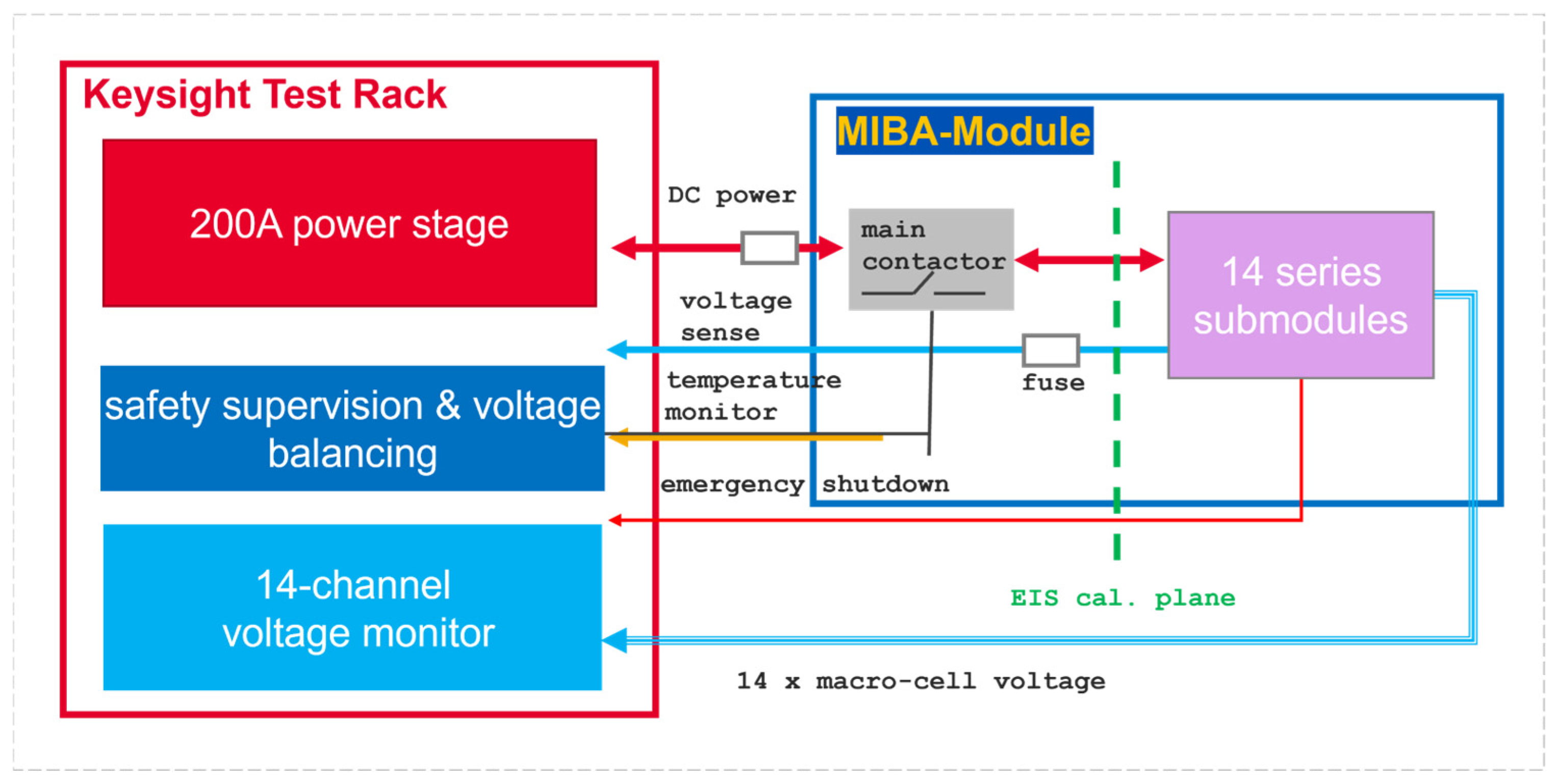
Figure 1 shows the battery measurement setup and test-system architecture for battery modules. The battery test hardware comprises a three-phase powered battery tester (Keysight SL1001A, Keysight Technologies, Santa Rosa, CA, USA) with voltage and current ratings of up to 100 V and 200 A, respectively. To connect the battery to the tester, a four-wire Kelvin connection with force and sense connections is used. The force wires are robust cables with a cross-sectional area of 100 mm2 to minimize Joule heat (I2R) losses. A safety supervision system is used to monitor individual cell voltages, current levels, and cell temperatures. In the event of any abnormal readings, the safety supervision system initiates a test shutdown, promptly disconnecting the battery via a high-power switch with an 80 kA rated service current. Communication to the battery submodule interface board is established through a 16-channel analog data acquisition interface. For single battery cell measurements, a cell tester (Keysight SL1007A, Keysight Technologies, Santa Rosa, CA, USA) was used, with a high sampling rate of 12.5 kHz. The tester is configured to handle voltages up to 6 V and currents up to ±25 A with high precision, providing a voltage resolution of 0.5 mV and a current measurement accuracy of ±0.05%.
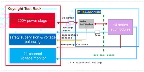
Figure 1.
Battery module test architecture and hardware setup. Conceptual overview of the test architecture with module test hardware and software systems, connected to the battery module (MIBA, 14S32P Bad Leonfelden). The test system comprises a three-phase powered tester and a multichannel analog data acquisition interface to monitor the individual submodule voltages. Arrow colors indicate signal types: red arrows denote bi-directional power flow, blue arrows show voltage sensing and monitoring connections, and yellow arrows represent temperature and safety signal paths.
2.2. Impedance Spectroscopy Calibration
In galvanostatic mode EIS, an alternating current (AC) sine wave signal is applied to the battery module and the system response is recorded, including the voltage drop v(t) across the module terminals and the current i(t) passing through it. Both signals are digitized simultaneously by a two-channel analog-to-digital converter at a sample rate of 1/Ts (Ts being the sample interval), ensuring that each sine wave is sampled at least 10 times, and the sine wave period is an integer multiple of Ts. To ensure the quality of the EIS data, at least one full sine wave is acquired per frequency, along with a predefined minimum time limit of 1 s. For example, in the case of the lowest frequency point at 50 mHz, only one full wave is recorded requiring 20 s. In the case of higher frequencies such as 10 Hz, it requires 0.1 s for one full wave period, thus 10 periods are recorded until the minimum time limit of 1 s is reached. Consequently, the number of sine wave periods captured varies with the frequency. A constant sampling rate is ensured resulting in a consistent energy per frequency and uniform energy distribution. The digitized signals, i(k) and v(k), undergo smoothing via a rectangular window of length N, which is selected such that the resulting signals include a specific number of full sinusoidal periods. This technique effectively avoids spectral leakage and ensures consistent measurements. Subsequently, the windowed signals are transformed into the frequency domain using a discrete Fourier transform. The resulting complex signals, i(ω) and v(ω), are used to compute the complex raw impedance, Z(ω)raw = v(ω)/i(ω). Figure 2 shows the impedance calibration process and the comparison of the calibrated EIS to the uncalibrated raw data. The measurement error model for EIS (Figure 2a) includes two components that contribute to the systematic error of the measured impedance (Zmd), a series impedance (Zser) and a complex gain (k) [10]. Therefore, two calibration measurements are necessary to obtain the complex gain factor k and the offset Zser, and to solve the calibration equation system. The first measurement is conducted with a short standard, while the second measurement is conducted with a shunt standard that has a known resistance value of 100 mΩ. The true impedance of the battery (Ztr) is then determined by Ztr = (Zmd − Zser)/k. A detailed description of the impedance calibration method is published in [10]. Figure 2b shows a Nyquist plot comparing the raw EIS data (blue) and the corrected data (red) across a frequency range of 50 mHz to 1 kHz, at 60% SoC and 23 °C. For the calibration, the sense voltage cables from the battery module are connected to a breakout box equipped with built-in calibration features. After the calibration, the force wires are reconnected to the battery module, while the sense wires are linked directly to the module via a switch in the calibration box. Thereby, the wires and fixtures are geometrically well positioned with a minimum of wire movements, resulting in a well-defined calibration plane, which is determined by the short-sense wires linking the sense box to the battery module.
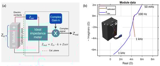
Figure 2.
Electrochemical Impedance Spectroscopy (EIS) calibration and data correction. (a) Schematic representation of the error model for the battery module test system, including an ideal impedance meter with a series error impedance Zser and a gain error coefficient k. (b) Raw (blue) and calibrated (red) EIS data are compared in a Nyquist plot ranging from 50 mHz to 1 kHz. The inset shows the 3.7 kWh battery module measured under ambient room temperature conditions and 60% SoC.
2.3. Time-Domain Pulse Analysis
A pulse current waveform pattern was applied to the battery module comprising a sequence of charge and discharge pulses of 10 A with pulse widths ranging from 20 to 80 s, followed by a recovery period of 260 s. The voltage response of the overall 14S32P battery module and its 14 submodules was recorded and analyzed by using a bilinear transformation applied to the response voltage vectors v(t) [27,28]. The approach involves three main steps. First, find a discrete solution for an RC filter. Thereby, measured current and voltage data are used to derive a discrete solution for the RC filter. The resulting coefficients are compared against a second-order transfer function. This step utilizes the Z-transform to achieve a linear mapping from the continuous Laplace domain to the discrete domain. Second, relaxation time constants are extracted from the pulse test data using the time-domain DRT. Third, the time-domain results are converted to the frequency domain for direct comparison with EIS data. In more detail, the three steps are as follows:
- Discrete solution of an RC filter
The time-continuous filter prototype with one parallel RC element in the Laplace domain is given as,
where H(s) is the transfer function in the continuous frequency domain, V(s) and I(s) are the voltage and current variables in the frequency domain, and s is the Laplace complex variable. Following reference [29], a prewarping scale in combination with a bilinear transformation is applied, resulting in
where ω0 is the desired cutoff frequency for the discrete filter in rads−1, Ts is the sampling time in seconds, and z is the Z-transform complex variable. Choosing a normalized cutoff frequency of u0 = 1 rads−1 and multiplying the numerator and denominator by z−1, s is written as follows:
Defining C1 as C1 = 1/tan (ω0 Ts/2), and substituting back into Equation (3), the RC filter response is formulated as
In the Z-domain, the input current and output voltage vectors of a filter can be represented by a second-order rational transfer function in the form,
Rearranging Equation (5) and comparing nominator and denominator coefficients with the coefficients in Equation (4), the filter coefficients a and b are identified as
For normalization we assume a(1) = 1. The time-domain discrete voltage response solution for a given current input sequence is calculated by applying the digital filter optimization method referred to as the Transposed II method’ recursively, as described in reference [30].
- b.
- Calculation of the time-domain distribution of the relaxation time (DRT)
To obtain the DRT from the time-domain data, the difference between Y(ω) and the experimental data Yexp (ω) is minimized by optimization of Xk representing the relaxation time constant vector for each kth RC element:
The open circuit voltage Yocv is added to the DRT voltage response to satisfy the offset of the measured cell voltage. Converting Equation (7) into a matrix form with the discrete values of u in a vector form of k elements, we get
where Xk is a column vector of resistances (), for normalization we consider = 1.
- c.
- Converting the time-domain results to the frequency domain
Finally, the impedance spectrum is reconstructed from the DRT data:
where Z(ωn) is the impedance at frequency n, f represents the frequency vector, and τk represents the kth element of the relaxation time vector.
2.4. Battery Module, Submodule, and Cells
The battery module (MIBA 14S32P) is comprised of 14 submodules arranged in series, with each submodule housing 32 individual cells connected in parallel, leading to a 14S32P architecture. In the battery module, a voltage breakout board is connected to the individual submodules for voltage monitoring and balancing, using a maximum current of 100 mA. The individual cells are cylindrical 26,650 lithium-ion power cells, consisting of a cathode composed of iron phosphate (LiFePO4, LFP) and a standard graphite anode (LiC6). Each cell has a nominal voltage of 3.3 V and a capacity of 2.5 Ah, equivalent to 8.25 Wh per cell. Consequently, the battery module has a total capacity of 80 Ah, a voltage rating of 46.2 V, and an overall rated energy of 3.7 kWh. The battery module is designed for industrial applications where fast charging of up to 4C rates in combination with a long cycle life of 2000+ cycles is needed. All EIS and pulse measurements were conducted at a stable ambient temperature of 23 °C. The low C-rate cycling protocol and inclusion of rest periods ensured minimal self-heating of the cells, such that temperature effects were considered negligible for the scope of this study.
3. Results and Discussion
3.1. Calibrated EIS and Pulse Tests
The 3.7 kWh battery module was characterized with calibrated EIS and pulse tests, and the data were fitted with an ECM. For the EIS calibration, the measurement process can be described by integrating an ideal impedance meter with a series error impedance Zser and a gain error coefficient k. The relationship between the measured impedance Zmd and the actual impedance Ztr is governed by the complex gain factor k and the offset Zser. The calibration process to obtain the actual impedance Ztr yields a significant improvement in EIS data accuracy, particularly at higher frequencies above 100 Hz (Figure 2b). The error which is the difference between the raw and corrected impedance becomes more pronounced with increasing frequency due to the inductive coupling between the force and sense wires. For example, at 1 kHz the error rises to 87% on the real part of the impedance. After the calibration process, the battery module was charged to 100% SoC at a low current rate of 0.1C. Throughout the charging process, both module and submodule voltages were monitored, and active balancing procedures were implemented to maintain voltages below a 5% deviation threshold. After reaching full charge, the module was left to rest for 24 h. Subsequently, spot measurements of EIS and pulse tests were performed at every 10% SoC step, ranging from 100% SoC to 0% SoC, using a 0.1C discharge current, followed by a 60-min rest period after each SoC step. In total, 11 EIS and pulse measurements were conducted across the SoC range (Figure 3).
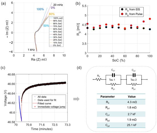
Figure 3.
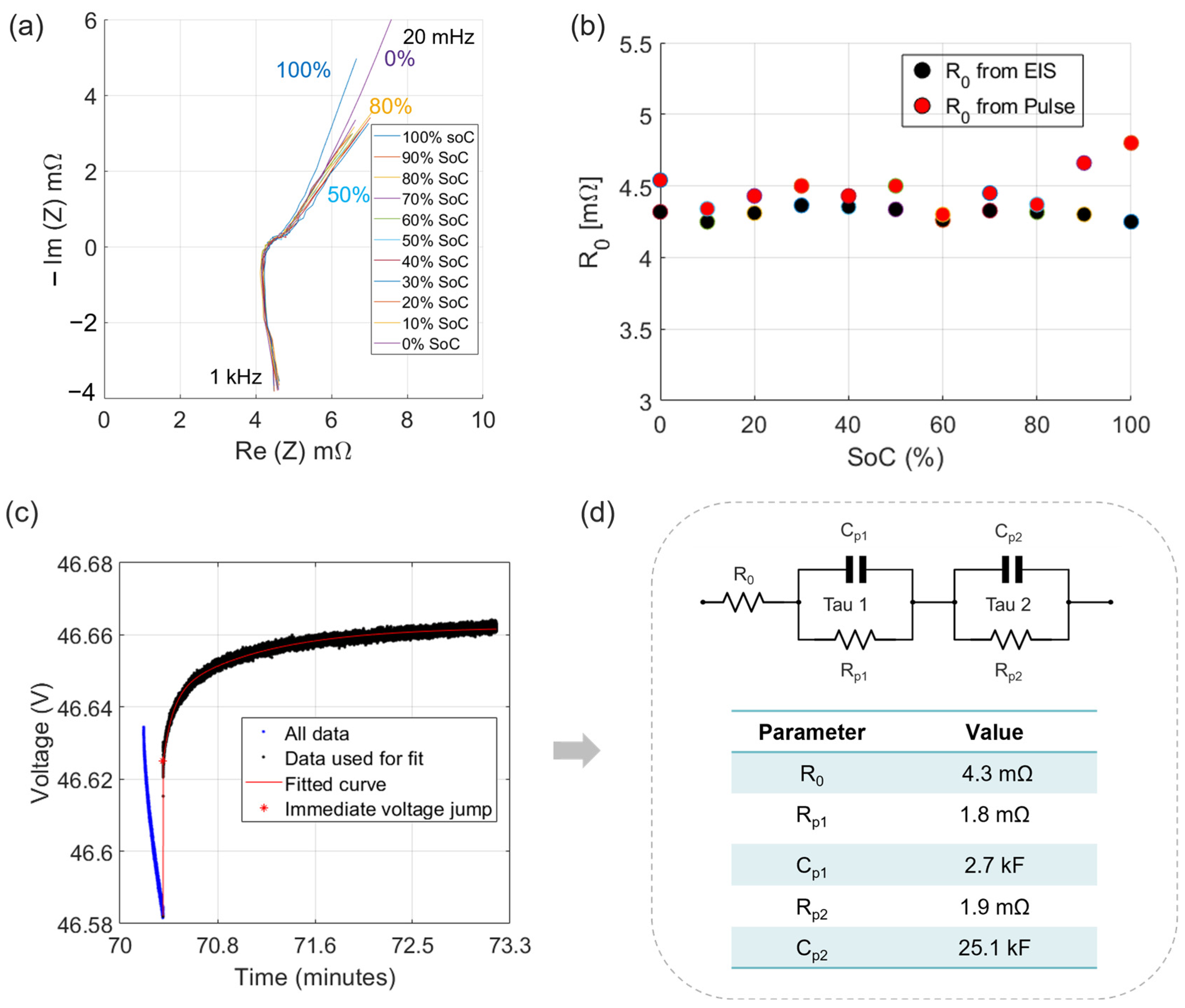
Module EIS and pulse tests, and ECM. (a) EIS spectra overlayed for various SoC levels, conducted in the discharge direction. (b) R0 determined from the EIS spectra by identifying the intersection point on the x-axis at approximately 200 Hz (black), and R0 determined from the pulse tests (red). (c) Pulse data. Voltage recovery from current pulse and model fit for the pulse at 60% SoC. (d) The ECM and the primary circuit parameters extracted from the fit.
Figure 3a shows the Nyquist plot of the EIS data collected at the module level at 11 SoC increments. Notably, the impedance spectra demonstrate minimal dependency on SoC, except at low frequencies below 1 Hz. Figure 3b shows the ohmic resistance parameter (R0) as derived from the x-axis intersection for EIS, ranging from R0 = 4.2 to 4.4 mΩ across different SoC levels. It is notable that no full ECM fitting was performed for the EIS spectra in Figure 3a, as the focus of this work is on reconstructing impedance spectra from time-domain pulse measurements. Only R0 was extracted and analyzed. Figure 3c shows the time-domain voltage response curve resulting from the 10 A discharge pulse test conducted at 60% SoC and the ECM fit applied to the time-domain pulse response data. The ECM consists of an ohmic resistance R0 and two RC circuits which are used to model the slow and the fast time constants of the voltage response curve, respectively (Figure 3d). From the voltage response curve, the immediate voltage jump was used to determine R0, while the exponential voltage rise determines the two-time constants τ1 and τ2. The ohmic resistance values R0 obtained from the pulse test at various SoC levels range from R0 = 4.3 to 4.8 mΩ, which are very close to R0 obtained from EIS (Figure 3b). While a good match is observed for R0 values, a slight deviation is observed at high SoC arising from the higher polarization of the battery, resulting in a slightly higher voltage drop during the pulse test. The fast time constant obtained from the ECM is τ1 = 4.8 s (related to charge transfer processes), and the slow time constant is τ2 = 47.6 s (related to slow diffusion processes).
3.2. Reconstruction of the Impedance Data from the Time-Domain Pulse
Figure 4 shows an overview of the approach to derive the time-domain DRT from the pulse data and reconstruct the corresponding EIS data. The DRT analysis of pulse tests involves several steps. Initially, transient current pulses are applied to the battery module, resulting in dynamic voltage responses (Figure 4, upper panel). The voltage responses are recorded and processed to extract relevant time-domain information, including the ohmic resistance R0. Subsequently, the acquired data undergo linear transformations and optimization steps as discussed in Section 2.3 to determine the distribution of relaxation times, providing insights into electrochemical processes across different timescales. As a final step, curves in the style of EIS measurements are reconstructed from the DRT data and compared to EIS measurements.
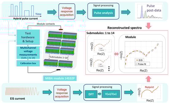
Figure 4.
Reconstruction of EIS data from time-domain pulse data. The upper panel displays the hybrid pulse current as the input waveform, along with the post-processing steps, from left to right as indicated by the arrows. The lower panel illustrates the conventional EIS method, including the signal processing to obtain the resulting Nyquist plot. The middle panels show the 14S32P module test with 14 series submodules, including the test hardware configuration, force, and sense wiring, and the EIS calibration box. The red box shows the reconstructed EIS for the entire module and for each of the 14 individual submodules.
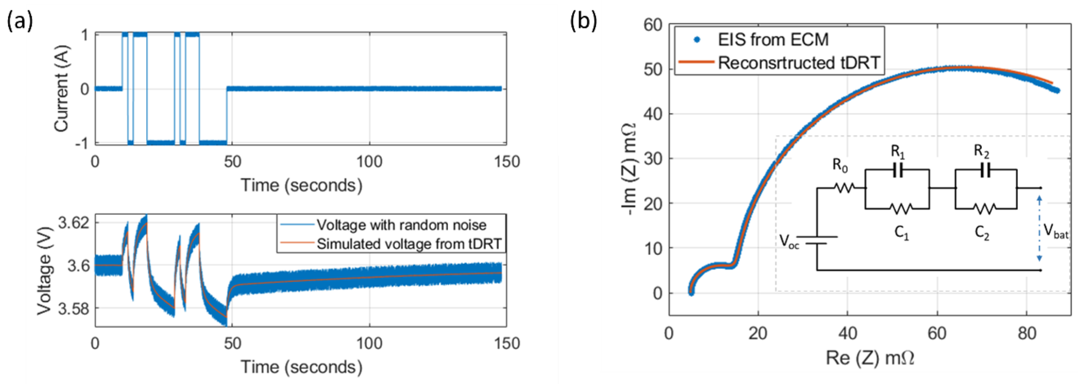
Figure 5 validates the EIS reconstruction using synthetic pulse data and simulated voltages. A time-domain pulse sequence was generated (Figure 5a) and fed into the ECM (Figure 5b, inset). The resulting voltage response was overlaid with random noise to simulate real-world conditions (Figure 5a). The DRT was calculated, and time-domain results were transformed to the frequency domain to reconstruct the EIS curves (Figure 5b). A good overlap is obtained between the EIS curves derived from the ECM and the reconstructed impedance from DRT, with a root-mean-square error below 0.15 mΩ. While the time-domain DRT method is applicable to a wide range of pulse sequences, the effectiveness of the reconstruction depends on the design of the current profile, including the use of appropriately spaced pulse widths, amplitudes, and rest periods to capture the relevant dynamic processes within the battery.
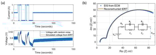
Figure 5.
Simulation results from the time-domain pulses and EIS reconstruction. (a) Current profile with hybrid pulse pattern (upper part) and simulated voltage with random noise (blue) and voltage generated from the DRT (lower part, red). (b) Nyquist plot with simulated EIS data (blue) and the ECM model used for simulation (inset); reconstructed impedance spectrum from the DRT (red).
Figure 6 presents the pulse data analysis, and the reconstructed EIS derived from the DRT analysis of a single battery cell. The measurements were conducted using a cell tester with a high sampling rate of 12.5 kHz. A peak current of 100 mA was applied during the pulse test (Figure 6a), and a total of 100 s of data were recorded for the reconstruction process. The corresponding voltage response of the cell is shown in Figure 6a, lower panel. The DRT data were computed and transformed into the frequency domain to reconstruct the EIS curves (Figure 6b). A good alignment of the reconstructed EIS curve is obtained with the experimentally measured EIS over a frequency range of 10 mHz to 1 kHz.
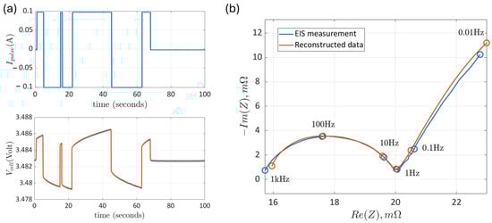
Figure 6.
Pulse data and reconstructed EIS curves from the DRT spectrum of a single battery cell using a cell tester with a high scan rate. (a) Pulse test current (upper, blue) and voltage response of the cell (lower, red). (b) Comparison of reconstructed EIS from the DRT analysis with measured EIS over a frequency range of 10 mHz to 1 kHz.
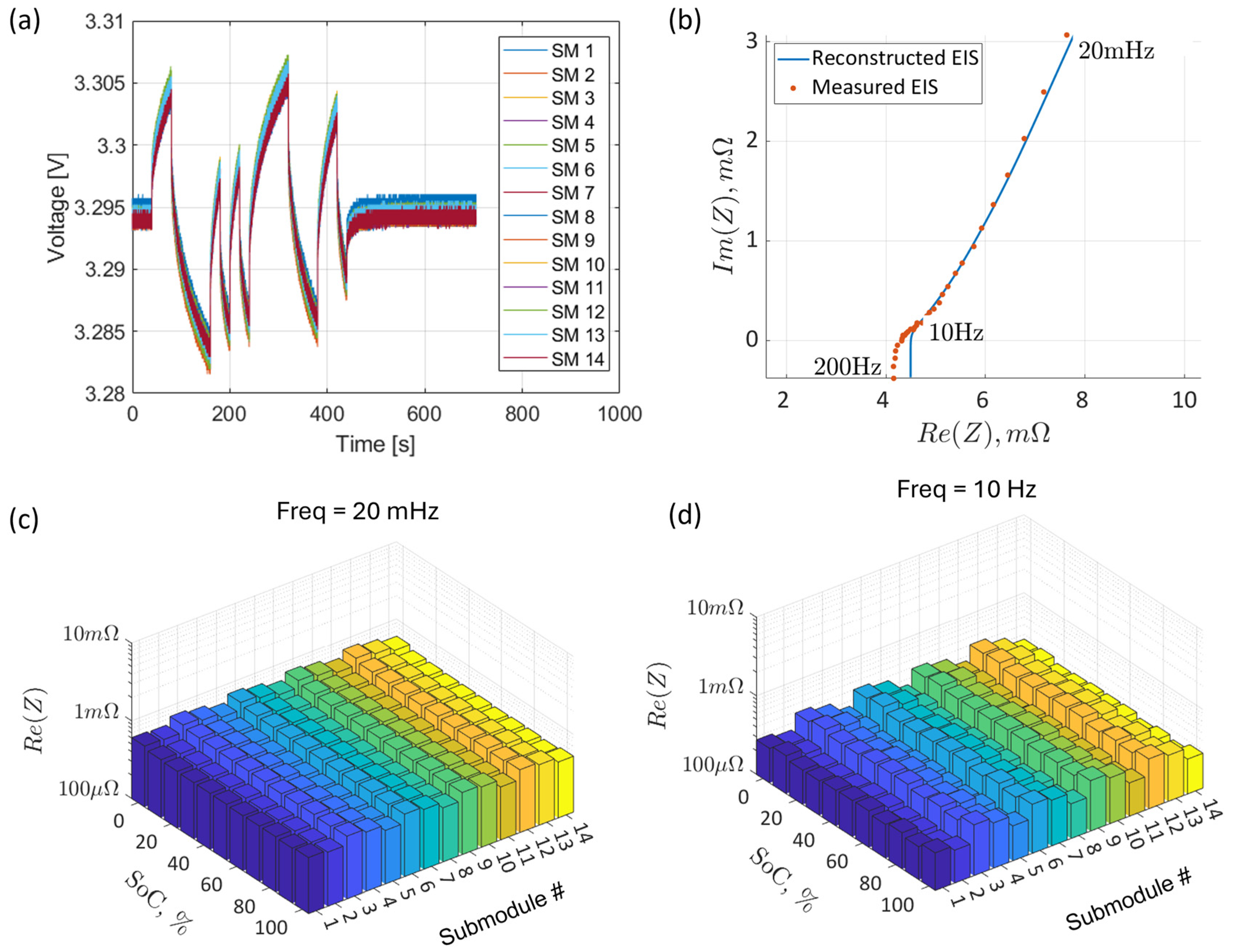
Figure 7 shows the pulse data analysis and reconstructed EIS from DRT data of the full battery module consisting of 14 battery submodules. A pulse current pattern was applied to the battery module, including 10A charge and discharge pulses with pulse widths ranging from 20 to 80 s, followed by a recovery period of 260 s. The voltage responses of the overall 14S32P battery module and its 14 submodules were recorded, with an average value of 46.14 V ± 70 mV (Figure 7a). The relaxation time-domain data were calculated and transformed to the frequency domain for reconstructing EIS curves (Figure 7b). The comparison with the measured EIS of the full module was conducted from 20 mHz to 200 Hz. While a close overlap was observed from the low to medium frequency range, some deviations emerged at high frequencies above 10 Hz. This is primarily attributed to the limited sampling rate of the measured voltage and current data, which limits the resolution of the high-frequency components. The EIS test lasted ~30 min, while the pulse test including the recovery periods required ~10 min. In Figure 7c, a 3D plot of the reconstructed impedance data is shown for the 14 submodules with respect to the SoC, at 20 mHz (left) and 10 Hz (right). In contrast to existing methods of DRT analysis [30], the method presented here uses measured current data instead of mathematical descriptions of current patterns. This enhances robustness against data anomalies such as system noise or spikes while providing greater versatility in handling various excitation current patterns. In addition, while standard DRT analysis uses a regularization technique for accurate interpretation, the presented approach does not require regularization as the DRT component is only an intermediate result towards the final complex impedance data.
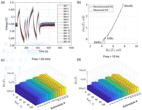
Figure 7.
Pulse data and reconstructed EIS curves from the DRT spectrum of the battery modules. (a) Voltage response for submodules 1 to 14, at 100% SoC. Several voltage traces visually overlap due to similar response characteristics, causing some individual colors to be indistinguishable in the plot (b) Comparison of reconstructed EIS from DRT analysis with measured EIS, with a 600 nH inductance added mathematically for alignment at 200 Hz, solely for comparison purposes. (c) Real part of the reconstructed EIS for the 14 submodules at different SoC, at 20 mHz (d) Real part of the reconstructed EIS for the 14 submodules at different SoC, at 10 Hz. Each submodule is indicated by one color.
4. Conclusions
We present an efficient method for reconstructing module EIS curves from time-domain pulses using an advanced time-domain DRT method. The method was demonstrated through a simulation experiment, as well as on a single battery cell with a capacity of 12 Wh, and on a battery module with a capacity of 3.7 kWh. Dynamic voltage responses were measured from the 14 submodules of a 14S32P module, and the ohmic resistance (R0) was determined from both the time-domain and frequency EIS spectra. Pulse tests were combined with DRT to reconstruct EIS curves of the 3.7 kWh 14S32P module across different SoCs. The reconstructed EIS curves closely match the calibrated EIS experiments, with a root-mean-square error below 0.15 mΩ (<0.25%). This method achieves a 67% reduction in measurement time compared to classical EIS methods, with pulse tests requiring only 10 min, compared to 30 min for EIS measurements in the frequency range of 50 mHz to 100 Hz. The time savings were achieved through the dynamic adjustment of the measurement sampling frequency in the time-domain approach, eliminating the need for a full sine wave per frequency point, as required in EIS. The proposed DRT method also enhances robustness by directly utilizing measured current data, rather than relying on numerically simulated current pattern descriptions typically used in traditional DRT methods. Moreover, the advanced DRT analysis improves the spectral resolution of time-domain data by deconvoluting overlapping signals into distinct relaxation time distributions. This separation provides a more comprehensive characterization of electrochemical processes that might otherwise remain indistinguishable.
Author Contributions
M.K.: Conceptualization, methodology, investigations, data analysis, data curation. M.M.: data analysis, discussion, writing—review, and editing. H.P.: resources (Battery module operation), discussion, review, and editing. F.K.: resources, supervision, conceptualization, writing of the original draft, discussion, funding acquisition. N.A.-Z.R.-S.: investigations, data curation, discussion, visualization, writing original draft preparation, review, and editing. All authors have read and agreed to the published version of the manuscript.
Funding
This work was partially funded by the project BatteryLife (project no. Wi-2022-603642) an FTI Initiative Kreislaufwirtschaft from the Upper-Austrian Government; and by the European Union Horizon project DigiCell under Grant Agreement no. 101135486.
Data Availability Statement
The original contributions presented in the study are included in the article; further inquiries can be directed to the corresponding authors.
Acknowledgments
The authors would like to thank Robert Mülleder for his work in bringing the battery modules into operation.
Conflicts of Interest
Author Hartmut Popp was employed by Miba Battery Systems GmbH, and authors Manuel Kasper, Manuel Moertelmaier, Ferry Kienberger, and Nawfal Al-Zubaidi R-Smith were employed by Keysight Laboratories, Keysight Technologies GmbH. All authors declare that the research was conducted in the absence of any commercial or financial relationships that could be construed as a potential conflict of interest.
References
- Liu, J.; Yadav, S.; Salman, M.; Chavan, S.; Kim, S.C. Review of thermal coupled battery models and parameter identification for lithium-ion battery heat generation in EV battery thermal management system. Int. J. Heat Mass Transf. 2024, 218, 124748. [Google Scholar] [CrossRef]
- Tashakor, N.; Naseri, F.; Fang, J.; Zadeh, A.H.; Goetz, S. Module Voltage and Resistance Estimation of Battery-Integrated Cascaded Converters Through Output Sensors Only for EV Applications. IEEE Trans. Transp. Electrif. 2024, 10, 7984–7995. [Google Scholar] [CrossRef]
- Dixon, J.; Bell, K. Electric vehicles: Battery capacity, charger power, access to charging and the impacts on distribution networks. eTransportation 2020, 4, 100059. [Google Scholar] [CrossRef]
- McGovern, M.E.; Bruder, D.D.; Huemiller, E.D.; Rinker, T.J.; Bracey, J.T.; Sekol, R.C.; Abell, J.A. A review of research needs in nondestructive evaluation for quality verification in electric vehicle lithium-ion battery cell manufacturing. J. Power Sources 2023, 561, 232742. [Google Scholar] [CrossRef]
- Galeotti, M.; Cinà, L.; Giammanco, C.; Cordiner, S.; Di Carlo, A. Performance analysis and SOH (state of health) evaluation of lithium polymer batteries through electrochemical impedance spectroscopy. Energy 2015, 89, 678–686. [Google Scholar] [CrossRef]
- R-Smith, N.A.-Z.; Leitner, M.; Alic, I.; Toth, D.; Kasper, M.; Romio, M.; Surace, Y.; Jahn, M.; Kienberger, F.; Ebner, A.; et al. Assessment of lithium ion battery ageing by combined impedance spectroscopy, functional microscopy and finite element modelling. J. Power Sources 2021, 512, 230459. [Google Scholar] [CrossRef]
- Xiong, R.; Pan, Y.; Shen, W.; Li, H.; Sun, F. Lithium-ion battery aging mechanisms and diagnosis method for automotive applications: Recent advances and perspectives. Renew. Sustain. Energy Rev. 2020, 131, 110048. [Google Scholar] [CrossRef]
- Gao, Y.; Jiang, J.; Zhang, C.; Zhang, W.; Ma, Z.; Jiang, Y. Lithium-ion battery aging mechanisms and life model under different charging stresses. J. Power Sources 2017, 356, 103–114. [Google Scholar] [CrossRef]
- Liu, Y.; Wang, L.; Li, D.; Wang, K. State-of-health estimation of lithium-ion batteries based on electrochemical impedance spectroscopy: A review. Prot. Control. Mod. Power Syst. 2023, 8, 1–17. [Google Scholar] [CrossRef]
- Kasper, M.; Leike, A.; Thielmann, J.; Winkler, C.; R-Smith, N.A.-Z.; Kienberger, F. Electrochemical impedance spectroscopy error analysis and round robin on dummy cells and lithium-ion-batteries. J. Power Sources 2022, 536, 231407. [Google Scholar] [CrossRef]
- Böttiger, M.; Paulitschke, M.; Bocklisch, T. Systematic experimental pulse test investigation for parameter identification of an equivalent based lithium-ion battery model. Energy Procedia 2017, 135, 337–346. [Google Scholar] [CrossRef]
- Białoń, T.; Niestrój, R.; Skarka, W.; Korski, W. HPPC Test Methodology Using LFP Battery Cell Identification Tests as an Example. Energies 2023, 16, 6239. [Google Scholar] [CrossRef]
- Wang, Y.; Kim, S.-Y.; Chen, Y.; Zhang, H.; Park, S.-J. An SMPS-Based Lithium-Ion Battery Test System for Internal Resistance Measurement. IEEE Trans. Transp. Electrif. 2023, 9, 934–944. [Google Scholar] [CrossRef]
- Zhang, M.; Liu, Y.; Li, D.; Cui, X.; Wang, L.; Li, L.; Wang, K. Electrochemical Impedance Spectroscopy: A New Chapter in the Fast and Accurate Estimation of the State of Health for Lithium-Ion Batteries. Energies 2023, 16, 1599. [Google Scholar] [CrossRef]
- Iurilli, P.; Brivio, C.; Wood, V. On the use of electrochemical impedance spectroscopy to characterize and model the aging phenomena of lithiumion batteries: A critical review. J. Power Sources 2021, 505, 229860. [Google Scholar] [CrossRef]
- Chan, H.S.; Dickinson, E.J.; Heins, T.P.; Park, J.; Gaberšček, M.; Lee, Y.Y.; Heinrich, M.; Ruiz, V.; Napolitano, E.; Kauranen, P.; et al. Comparison of methodologies to estimate state-of-health of commercial Li-ion cells from electrochemical frequency response data. J. Power Sources 2022, 542, 231814. [Google Scholar] [CrossRef]
- Kalogiannis, T.; Hosen, S.; Sokkeh, M.A.; Goutam, S.; Jaguemont, J.; Jin, L.; Qiao, G.; Berecibar, M.; Van Mierlo, J. Comparative Study on Parameter Identification Methods for Dual-Polarization Lithium-Ion Equivalent Circuit Model. Energies 2019, 12, 4031. [Google Scholar] [CrossRef]
- Moradpour, A.; Kasper, M.; Hoffmann, J.; Kienberger, F. Measurement Uncertainty in Battery Electrochemical Impedance Spectroscopy. IEEE Trans. Instrum. Meas. 2022, 71, 1006209. [Google Scholar] [CrossRef]
- Meddings, N.; Heinrich, M.; Overney, F.; Lee, J.-S.; Ruiz, V.; Napolitano, E.; Seitz, S.; Hinds, G.; Raccichini, R.; Gaberšček, M.; et al. Application of electrochemical impedance spectroscopy to commercial Li-ion cells: A review. J. Power Sources 2020, 480, 228742. [Google Scholar] [CrossRef]
- Moradpour, A.; Kasper, M.; Kienberger, F. Quantitative Cell Classification Based on Calibrated Impedance Spectroscopy and Metrological Uncertainty. Batter. Supercaps 2023, 6, e202200524. [Google Scholar] [CrossRef]
- Huang, X.; Li, Y.; Acharya, A.B.; Sui, X.; Meng, J.; Teodorescu, R.; Stroe, D.-I. A Review of Pulsed Current Technique for Lithium-ion Batteries. Energies 2020, 13, 2458. [Google Scholar] [CrossRef]
- Barai, A.; Uddin, K.; Widanage, W.D.; McGordon, A.; Jennings, P. A study of the influence of measurement timescale on internal resistance characterisation methodologies for lithium-ion cells. Sci. Rep. 2018, 8, 21. [Google Scholar] [CrossRef] [PubMed]
- Zhang, Q.; Wang, D.; Schaltz, E.; Stroe, D.-I.; Gismero, A.; Yang, B. Degradation mechanism analysis and State-of-Health estimation for lithium-ion batteries based on distribution of relaxation times. J. Energy Storage 2022, 55, 105386. [Google Scholar] [CrossRef]
- Goldammer, E.; Kowal, J. Determination of the Distribution of Relaxation Times by Means of Pulse Evaluation for Offline and Online Diagnosis of Lithium-Ion Batteries. Batteries 2021, 7, 36. [Google Scholar] [CrossRef]
- Plank, C.; Rüther, T.; Jahn, L.; Schamel, M.; Schmidt, J.P.; Ciucci, F.; Danzer, M.A. A review on the distribution of relaxation times analysis: A powerful tool for process identification of electrochemical systems. J. Power Sources 2024, 594, 233845. [Google Scholar] [CrossRef]
- Wang, J.; Huang, Q.-A.; Li, W.; Wang, J.; Bai, Y.; Zhao, Y.; Li, X.; Zhang, J. Insight into the origin of pseudo peaks decoded by the distribution of relaxation times/ differential capacity method for electrochemical impedance spectroscopy. J. Electroanal. Chem. 2022, 910, 116176. [Google Scholar] [CrossRef]
- Oppenheim, A.V.; Schafer, R.W.; Buck, J.R. Discrete-Time Signal Processing, 2nd ed.; Prentice-Hall Signal Processing Series; Prentice Hall: Upper Saddle River, NJ, USA, 1999. [Google Scholar]
- Tan, L.; Jiang, J. Chapter 6—Digital Signal Processing Systems, Basic Filtering Types, and Digital Filter Realizations. In Digital Signal Processing, 2nd ed.; Tan, L., Jiang, J., Eds.; Academic Press: Boston, MA, USA, 2013; pp. 161–215. [Google Scholar] [CrossRef]
- Parks, T.W.; Burrus, C.S. Digital Filter Design; Wiley: New York, NY, USA, 1987. [Google Scholar]
- Schmidt, J.P.; Ivers-Tiffée, E. Pulse-fitting—A novel method for the evaluation of pulse measurements, demonstrated for the low frequency behavior of lithium-ion cells. J. Power Sources 2016, 315, 316–323. [Google Scholar] [CrossRef]


Disclaimer/Publisher’s Note: The statements, opinions and data contained in all publications are solely those of the individual author(s) and contributor(s) and not of MDPI and/or the editor(s). MDPI and/or the editor(s) disclaim responsibility for any injury to people or property resulting from any ideas, methods, instructions or products referred to in the content. |
© 2025 by the authors. Licensee MDPI, Basel, Switzerland. This article is an open access article distributed under the terms and conditions of the Creative Commons Attribution (CC BY) license (https://creativecommons.org/licenses/by/4.0/).