AI-Based Prediction of Numerical Earthquakes Using (Pseudo) Acoustic Emission

Abstract

The Discrete Element Method is widely used in applied mechanics, particularly in situations where material continuity breaks down (fracturing, crushing, friction, granular flow) and classical rheological models fail (phase transition between solid and granular). In this study, the Discrete Element Method was employed to simulate stick–slip cycles, i.e., numerical earthquakes. At 2000 selected, regularly spaced time checkpoints, parameters describing the average state of all particles forming the numerical fault were recorded. These parameters were related to the average velocity of the particles and were treated as the numerical equivalent of (pseudo) Acoustic Emission. The collected datasets were used to train the Random Forest and Deep Learning models that successfully predicted the time to failure. SHapley Additive exPlanations (SHAP) was used to quantify the contribution of individual physical parameters of the particles to the prediction results. The main novelty of this study was the prediction of time to failure for entire event sequences. Using only instantaneous particle velocity statistics and without using information about the history of previous events, coefficients of determination in the range R² = 0.81–0.96 were obtained.

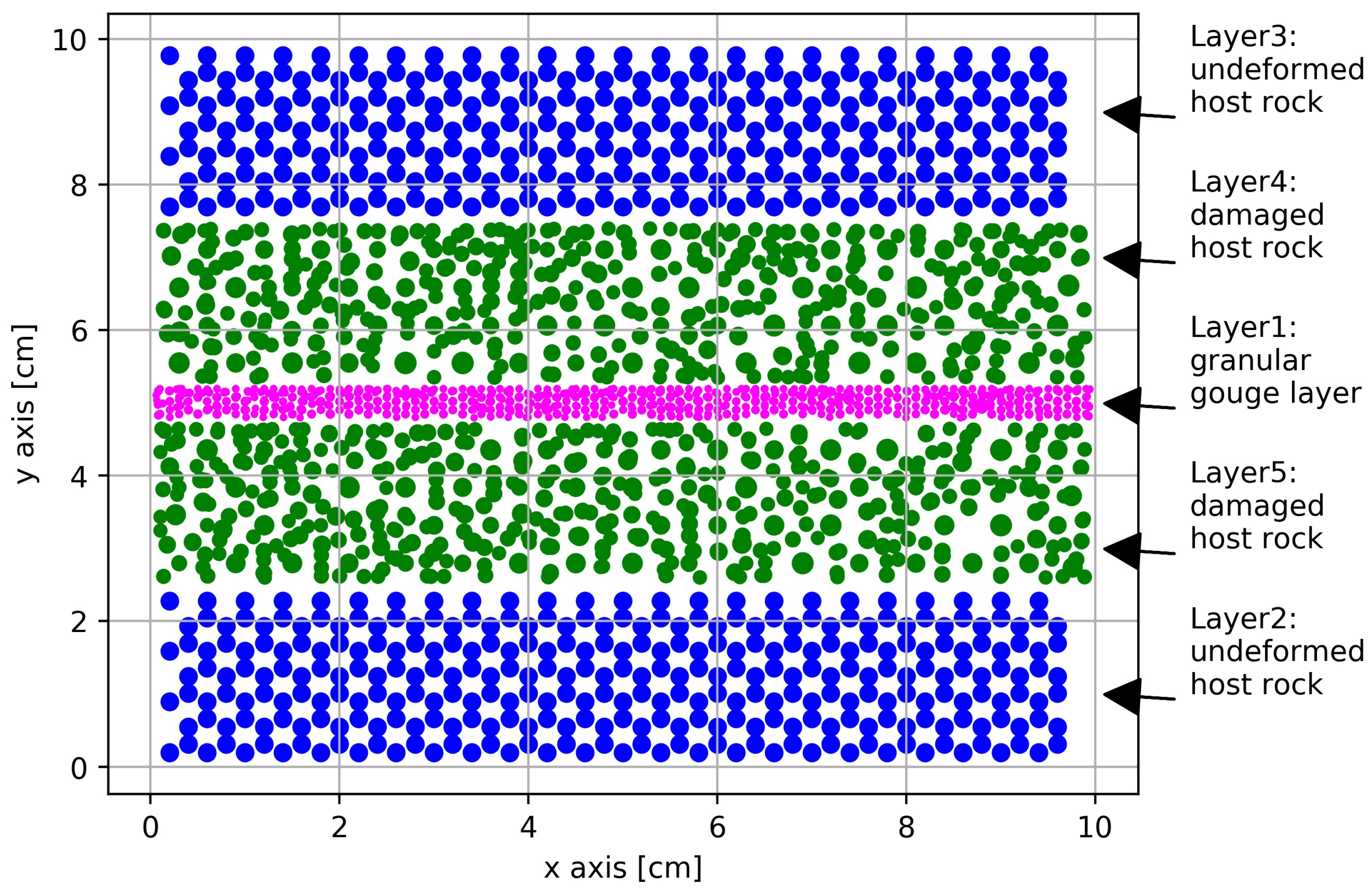
1. Introduction

Earthquakes are extremely complex geophysical phenomena. Despite decades of research, the processes governing earthquake initiation remain only partially understood. To date, no universal principle has been developed that would allow reliable prediction of the time and magnitude of future seismic events [1]. Short-term deterministic earthquake prediction is currently considered impossible. The general pattern of earthquake occurrence can, however, be described by stick–slip cycles [2]: periods of stress accumulation (stick) are followed by abrupt stress release (slip), reflecting the fundamental dynamics of seismic events.

Among the methods aimed at advancing the understanding of seismic phenomena, acoustic emission (AE) plays a particularly important role. AE can provide insight into processes occurring within fault zones. However, the relationship between acoustic energy and failure in the fault zone remains insufficiently understood. AE arises from material deformation and microcracking, releasing energy that propagates through the material as elastic waves. Owing to its versatility and non-destructive nature, AE is widely used for continuous real-time monitoring of fracture processes.

A major difficulty in earthquake physics research is the lack of sufficient direct observational data, since access to fault zones is limited. Laboratory experiments and numerical simulations can partially address this issue. In modeling failure processes, the Discrete Element Method (DEM) is particularly useful, as it enables tracking the motion of individual particles, interparticle forces, and process dynamics [3]. The DEM is particularly well suited for simulating stick–slip phenomena and so-called numerical earthquakes, as it represents granular media as inherently discontinuous systems in which deformation, stress accumulation, and abrupt stress release arise directly from local grain-scale interactions. In contrast to continuum-based approaches, where frictional instability is imposed through assumed constitutive laws, DEM allows stick–slip cyclicity, event irregularity, and the statistical character of slip events to emerge naturally from contact dynamics, force-chain reorganization, and local kinematic fluctuations. However, numerical simulations, especially those based on DEM, generate extensive datasets. Machine learning algorithms can effectively analyze such data, identifying hidden linear and nonlinear relationships, and opening new perspectives for earthquake research.

In several recent years, some studies have explored laboratory and numerical investigations of earthquakes, often combining acoustic emission analysis with machine learning techniques. A pioneering study by [4] demonstrated, using laboratory earthquake models, that supervised machine-learning algorithms trained on acoustic signals from stick–slip cycles can accurately predict the timing of subsequent slips. It was confirmed [5] that acoustic emission enables the prediction of both the timing and magnitude of laboratory earthquakes. Supervised learning methods have also contributed to the development of next-generation high-quality earthquake catalogs [6,7]. The Discrete Element Method was employed to predict macroscopic friction based on signals from individual particles [8]. In [9], it was shown that laboratory stick–slip shear experiments replicate the dynamics of natural earthquakes. When sufficient fault dynamics data are available, LightGBM, together with the SHAP value approach, was capable of accurately predicting the friction state of laboratory faults and the most critical input features for laboratory earthquake prediction [10]. Machine learning was also used [11] to show that statistical features of plate motion signals contain information about the slip duration and friction drop of laboratory earthquakes. The Isolation Forest algorithm from unsupervised machine learning was able to detect anomalies [12] in the numerical DEM model of stick–slip cycles. A DEM model was proposed [13] that takes into account an irregular, random pattern of stress increase and decrease in such a system to predict subsequent stick–slip events. In [14], an advanced machine learning was applied to meter-scale laboratory data and demonstrated that a trained model, using a network representation of the event catalog, can accurately predict the time to failure of mainshocks, from tens of seconds to milliseconds before occurrence.

This work is a continuation and complement to the work mentioned above. Here, a DEM model was presented that reproduces stick–slip cycles, hereinafter referred to as numerical earthquakes. Prior studies have demonstrated that machine learning can predict the time to failure of laboratory stick–slip events using features extracted from acoustic or active seismic signals recorded at the boundary. Complementary numerical work has shown that statistical features of particle-velocity signals in simulated sheared granular faults contain information about the global frictional state and intermittent stick–slip dynamics. Building on these directions, the present study focuses on a controlled DEM stick–slip system and links instantaneous, state-based descriptors derived from particle kinematics directly to the time-to-failure target. Based on continuous (pseudo) Acoustic Emission monitoring, machine learning models—Random Forest and Deep Learning—were trained. The main goal was to predict the time to failure between successive numerical earthquakes.

The applied numerical approach has inherent limitations arising both from the nature of the discrete element method and from the simplifying assumptions adopted in the model. It is emphasized that the primary reference of this study is not natural earthquakes, but laboratory stick–slip experiments, often referred to as laboratory earthquakes. The model represents a highly idealized granular system and neglects several processes that are essential at geological scales, including elastic wave propagation, material heterogeneity, thermal effects, pore-fluid interactions, and complex fault geometry. The temporal and spatial scales of the simulations are orders of magnitude smaller than those associated with natural seismicity, which precludes any direct transfer of the obtained results to real tectonic faults. In this context, the proposed methodology is not intended for direct analysis or forecasting of natural earthquakes. Its applicability is restricted to the investigation of frictional instability mechanisms and the testing of predictive methodologies under controlled conditions corresponding to laboratory and numerical earthquake models. In this study, laboratory stick–slip systems constitute the primary point of reference, while natural seismic phenomena provide a broader physical context and motivation rather than a direct target of analysis.

2. Materials and Methods

2.1. Discrete Element Method

A fault model capable of reproducing stick–slip cycles was developed. Its construction employed the DEM introduced by [3]. DEM is a particle-based numerical approach used to simulate brittle and granular materials, in which the material is represented as an assembly of interacting discrete elements. The method enables analysis of the translation and rotation of each particle at every time step, where translational motion is governed by Newton’s equations of motion, integrated using a conventional molecular dynamics scheme. The number of particles depends on the model geometry and the packing algorithm, in which larger particles are placed first, and smaller ones subsequently fill the remaining voids. DEM models allow investigation of processes inaccessible to laboratory observation, providing detailed information on each particle throughout the simulation.

The general workflow of a DEM simulation involves preparing the model geometry, followed by execution of the program’s main computational loop. At each iteration, particle contacts are detected, interparticle forces and resulting displacements are computed, and the geometry is updated. This cycle repeats until the simulation is completed. At every time step, Newton’s second law is applied to all discrete elements to compute position and velocity changes induced by acting forces. Numerical stability is satisfied by the Courant time-step criterion [15,16], to have particle displacements sufficiently small. DEM was computationally demanding, and modeling complex phenomena requires simplifications to achieve reasonable computation times [17].

One of the most widely used DEM implementations is the open-source software ESyS-Particle-3.0-alpha [18,19,20,21], employed in this study. Its main advantages include a parallel computing engine based on the Message Passing Interface (MPI) and a broad range of implemented particle interaction types.

2.2. Numerical Model of a Fault

The proposed model measured 10 cm × 10 cm × 1 cm and consisted of 2465 particles subjected to frictional interactions (Figure 1). Periodic boundary conditions were applied along the x-axis. The model was divided into horizontal layers with different properties, schematically representing the real fault structure [22]. The uppermost and lowermost layers represented undeformed host rock and consisted of particles with a radius of 0.2 cm. Two intermediate layers, representing damaged host rock, contained particles with radii from 0.1 to 0.3 cm. At the model center, a granular layer composed of particles with radii between 0.05 and 0.1 cm was introduced. Other researchers have employed DEM or FDEM fault models of comparable size [8,22,23].

The model was bounded at the top and bottom by rigid walls. A compressive force was applied along the y-axis, and a shear force acted along the x-axis. The simulation consisted of 200,000 time steps. The following unit system was adopted: length unit l = 1 cm, force unit F = 1 mN, and time unit t = 0.01 s. From these base units, derived quantities were defined: velocity v = l/t = 100 cm/s and mass m = 0.01 g.

Mature faults typically contain a granular layer formed by frictional wear and rock fragmentation. This layer significantly affects fault dynamics, stress distribution, and energy release processes [22,24,25]. Therefore, its presence was incorporated into the model.

Due to the high computational cost, the developed model is a simplified representation of a natural fault. Previous studies have shown that stick–slip phenomena in both experimental and numerical models follow the Gutenberg–Richter law and exhibit comparable b-values [24,26]. Furthermore, refs. [27,28] demonstrated that earthquakes exhibit fractal characteristics, meaning that processes occurring at millimeter and centimeter scales are similar to those at meter and kilometer scales [29]. This justifies the use of small-scale laboratory and numerical models in earthquake research.

In fault zones, the grain-size distribution typically follows a power-law relationship, with a small number of large particles and a large number of smaller ones [30]. The presented DEM model exhibits a grain-size distribution within its internal layers comparable to that observed in natural fault zones (Figure 2).

2.3. Machine Learning

Supervised Machine Learning and Deep Learning are widely applied to regression tasks. Classical supervised machine learning algorithms are effective for small- to medium-sized structured datasets, offering low computational cost. In contrast, DL models perform better on large, complex datasets, and their interpretability is more challenging. In the present study, the performance of both approaches was tested in a regression problem.

Supervised machine learning algorithm Random Forest (RF) was validated in similar studies [8,13,14]. RF consists of an ensemble of independent decision trees whose combined output forms the final prediction, applicable to both regression and classification tasks. By aggregating multiple trees, RF mitigates bias and overfitting typical of individual models. As an ensemble learning method, RF employs bootstrap aggregating (bagging), where multiple bootstrap samples are drawn with replacement from the original dataset. Each tree is trained independently. The final prediction is obtained by averaging individual tree outputs (for regression) or majority voting (for classification). Feature randomness further enhances model robustness. Effective RF performance requires tree independence, sufficient data diversity, and balanced tree depth. The algorithm tolerates randomly distributed noise but is sensitive to systematic errors. Although computationally slower and less interpretable than a single decision tree, RF substantially reduces overfitting, producing lower variance and prediction error. In this study, a Random Forest Regressor was implemented, and it constructed 500 regression trees using bagging with random feature selection at each split (max_features = “auto”), a fixed random seed (random_state = 42) for reproducibility, and parallel training (n_jobs = −1) to utilize all CPU cores.

A Deep Learning (DL) model was implemented using the Keras Sequential API [31,32,33], which represents a strictly feed-forward architecture where layers are stacked linearly, and data flow proceeds from the first layer to the last without branching or skip connections. Sequential models are particularly suitable for tabular regression tasks in which fully connected (dense) layers are sufficient to model nonlinear interactions between variables. The network consisted of two hidden layers with 64 neurons each, using the ReLU activation function to introduce nonlinearity and mitigate vanishing gradient effects. The output layer contained a single linear neuron to match the continuous nature of the regression target. Optimization was performed using the Adam algorithm with default hyperparameters, minimizing the mean squared error (MSE) loss. The network was trained for 120 epochs with a batch size of 32, using a 20% validation split. All input features were standardized via normalization (StandardScaler), ensuring stable gradient propagation and improving convergence.

2.4. Model Training, Testing, and SHAP-Based Evaluation

Some algorithms are sensitive to differences in feature magnitude and therefore require preprocessing through normalization or standardization, like DL. In contrast, tree-based models such as RF are inherently scale-invariant, eliminating the need for feature scaling. The dataset was divided into a training dataset (80%) and a testing dataset (20%); the model was trained on the training dataset to learn data relationships and evaluated on the testing dataset to assess predictive performance. To further minimize the risk of underfitting or overfitting, K-Fold Cross-Validation was applied, in which the dataset is partitioned into K folds (5-Fold in this case). Each fold serves once as a validation set, while the remaining folds are used for training. Model performance in the regression task was assessed using three standard metrics: the Coefficient of Determination (R²), Mean Absolute Error (MAE), and Mean Squared Error (MSE).

The influence of input features on the target variable was analyzed using SHapley Additive exPlanations (SHAP), a unified framework for model interpretability based on Shapley values from cooperative game theory [34]. SHAP quantifies the contribution of each feature to a model’s prediction, providing consistent additive explanations at both the local (individual prediction) and global (overall feature importance) levels. For tree-based models such as Random Forests, the TreeSHAP implementation enables fast and exact computation of Shapley values, making SHAP an effective method for interpreting complex ensemble models.

3. Results

3.1. Detailed Simulation Settings

Four experiments were carried out: Experiment 1 (E1), Experiment 2 (E2), Experiment 3 (E3), and Experiment 4 (E4). The same DEM model described above was employed in each case. A Normal Confining Force (NFC) of 0.4 mN was applied, and the Shearing Velocity (SV) was set to 2 cm/s. The thickness of the granular layer was 0.5 cm. 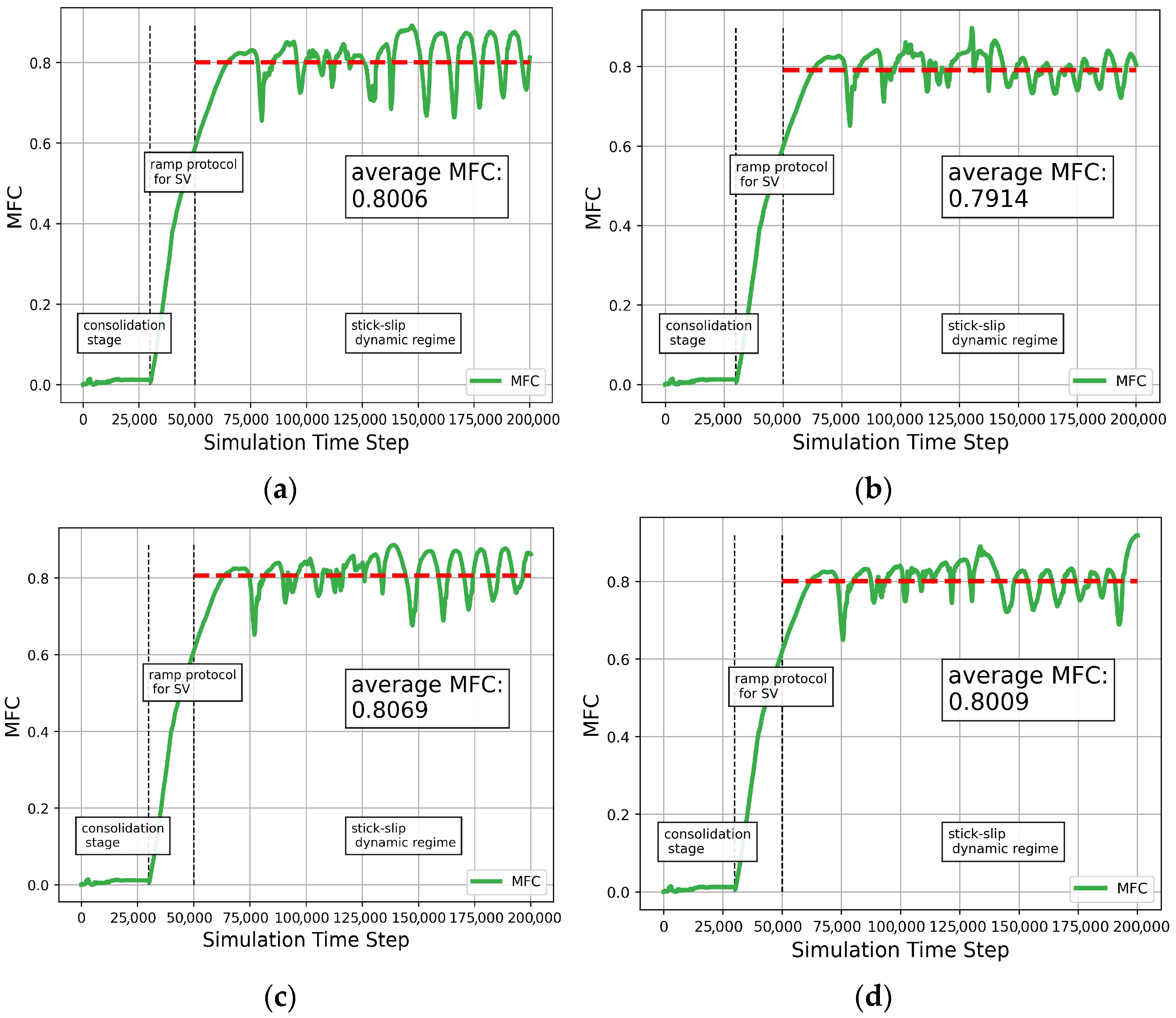Each experiment used a different particle density: E1—2.6 g/cm³ (2600 kg/m³), E2—2.7 g/cm³ (2700 kg/m³), E3—2.8 g/cm³ (2800 kg/m³), and E4—2.9 g/cm³ (2900 kg/m³). These densities are comparable to those of typical crustal rocks. In each simulation, the Macroscopic Friction Coefficient (MFC) was measured. The dimensionless MFC was defined as the ratio of the shear force [mN] to the normal force [mN] at each simulation time step. The final, average MFC value (aMFC) was obtained as the mean of all MFC values recorded after the consolidation phase (Figure 3). Although density does not directly affect the friction coefficient, it may exert an indirect influence through its impact on mechanical properties. By varying the density values across the four experiments, distinct MFC curve patterns were obtained during the simulations (Figure 3). Data collected during each simulation was used for training and testing machine learning algorithms. Each simulation comprised 200,000 time steps. The time step values were as follows: E1 − t1 = 0.0000213 s; E2 − t2 = 0.0000217 s; E3 − t3 = 0.0000221 s; and E4 − t4 = 0.0000225 s. The total simulated durations were E1—4.26 s; E2—4.34 s; E3—4.42 s; and E4—4.50 s.

3.2. MFC Curves During Stick–Slip Cycles

During the simulation (Figure 3), both the NFC and the SV were initially set to zero. The NFC increased linearly from 0 to the target value of 0.4 N over the time-step interval 0–5000, representing the consolidation period. Thereafter, NFC remained constant until the end of the simulation. The SV increased from 0 to 2 cm/s between time steps 30,000 and 40,000, following the so-called ramp protocol, and then remained constant for the remainder of the simulation. The MFC was computed at each time step. For each simulation, aMFC was calculated only after the consolidation period and ramp protocol, that is, for the time-step interval 50,000–200,000, referred to as the Simulation Interval (SI). The following aMFC values were obtained (Figure 3): E1—aMFC = 0.8006; E2—aMFC = 0.7914; E3—aMFC = 0.8069; and E4—aMFC = 0.8009.

The data used for training and testing the machine learning algorithms were collected over the same time-step interval SI. The objective of applying machine learning algorithms was to predict the Time to Failure (TtF). The TtF was determined based on the first derivative of MFC within SI. Increases in MFC values were interpreted as the stick phase, whereas decreases corresponded to the slip phase. The TtF was defined as the time between consecutive sign changes in the first derivative from negative to positive—that is, the moment when MFC stopped decreasing and began to increase. This transition corresponds to the end of a slip phase and the start of a stick phase. Each interval between two successive changes in the derivative’s sign from negative to positive was treated as an individual numerical earthquake event. The duration of the slip phase was assumed to be relatively short compared to the stick phase; therefore, the TtF was measured from the beginning of the stick phase to the end of the subsequent slip phase.

3.3. (Pseudo) Acoustic Emission

As shown in Figure 3, the stick–slip cycles in each experiment exhibited irregular and unique characteristics. The aim was to predict the TtF not based on the history of previous cycles, but through continuous monitoring of the state of particles forming the numerical fault. During the simulation, four parameters were recorded at each time step (

Table 1. Features used for Time to Failure predictions.

Feature1	Feature2
vx_m	vy_m
mean of the X component	mean of the Y component
of the particles’ velocity	of the particles’ velocity
Feature3	Feature4
vx_s	vy_s
standard deviation	standard deviation
of the X component of the particles’ velocity	of the Y component of the particles’ velocity

): the mean X component of particle velocity (vx_m), the mean Y component of particle velocity (vy_m), the standard deviation of the X component (vx_std), and the standard deviation of the Y component (vy_std).

Because local variations may not be reflected in mean values, the standard deviation was also included. These parameters were treated as (pseudo) Acoustic Emission (PAE). It was demonstrated [25] that in DEM simulations of stick–slip cycles, PAE can be effectively derived from quantities related to particle velocity.

3.4. Kinetic Energy Changes

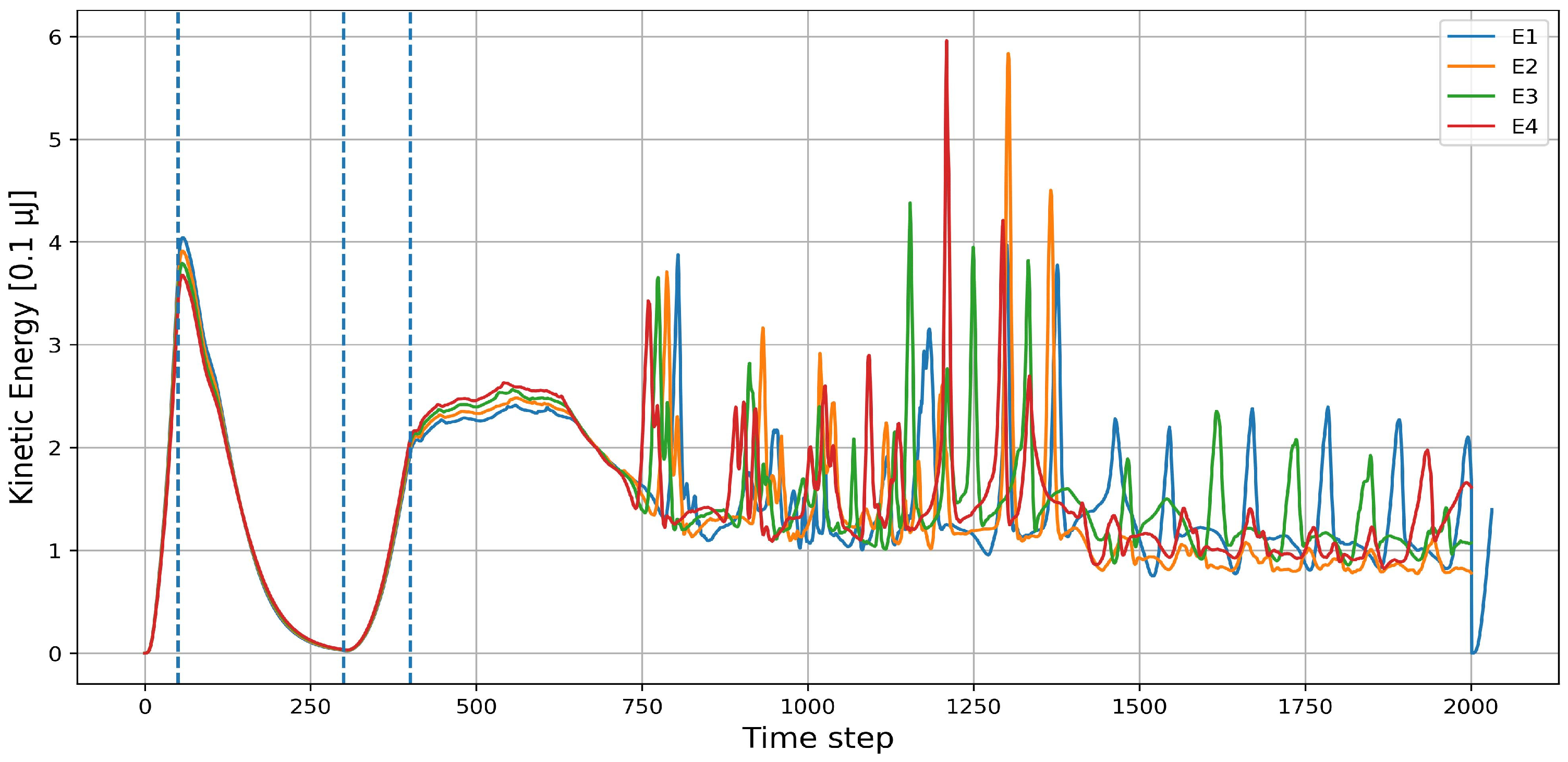
The kinetic energy plot (Figure 4) from the four DEM simulations exhibits a characteristic, irregular sequence of peaks with varying amplitudes, typical of stick–slip cycles. The periods of NCF activation, corresponding to time steps 0–5000, are marked with vertical dashed lines. The linear increase in the applied NCF value was accompanied by a proportional rise in kinetic energy. Between time steps 5000 and 30,000, the kinetic energy decreased nearly to zero, as the NCF no longer induced particle motion. In the interval between time steps 30,000 and 40,000, the SV was initiated and increased linearly. After time step 40,000, the main simulation phase commenced. When the system entered stick–slip mode, alternating phases were observed: periods of stopped motion, corresponding to stress accumulation during the stick–slip phase, and sharp, sudden peaks of kinetic energy, corresponding to slip events.

The distribution of peak amplitudes qualitatively resembles the Gutenberg–Richter law, in which small events occur much more frequently than large ones, while occasional extreme values correspond to major events. Overall, the results indicate that the presented numerical model reproduces, in an approximate manner, the key statistical and dynamic characteristics observed in laboratory-scale earthquakes.

3.5. TtF Prediction Methodology

During the simulation, so-called checkpoints were established within the SI at every hundredth time step. This approach, known as the moving time window technique, was used to record PAE at each checkpoint. Data were not collected at every time step in order to avoid excessive data accumulation. In each of the experiments E1–E4, approximately 1 GB of data was collected in total. For comparison, collecting data at every second time step would have resulted in approximately 150 GB per simulation. The collected data were used to train a supervised machine learning algorithm RF and a DL neural network. The parameters (features) associated with PAE were treated as dependent variables, while the TtF was defined as the independent variable. Predictions were made solely based on continuous monitoring of PAE from individual time windows, so the models generated forecasts without utilizing the history of previous events.

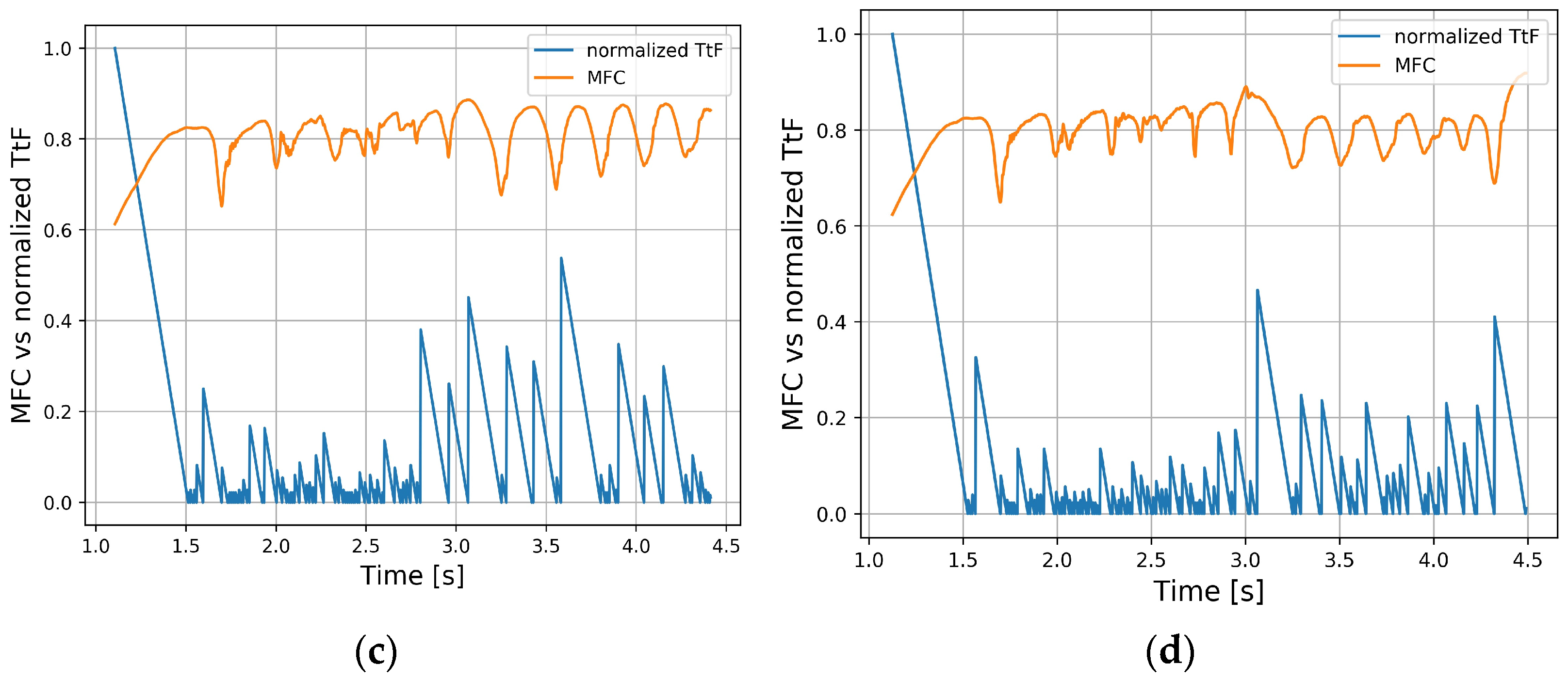
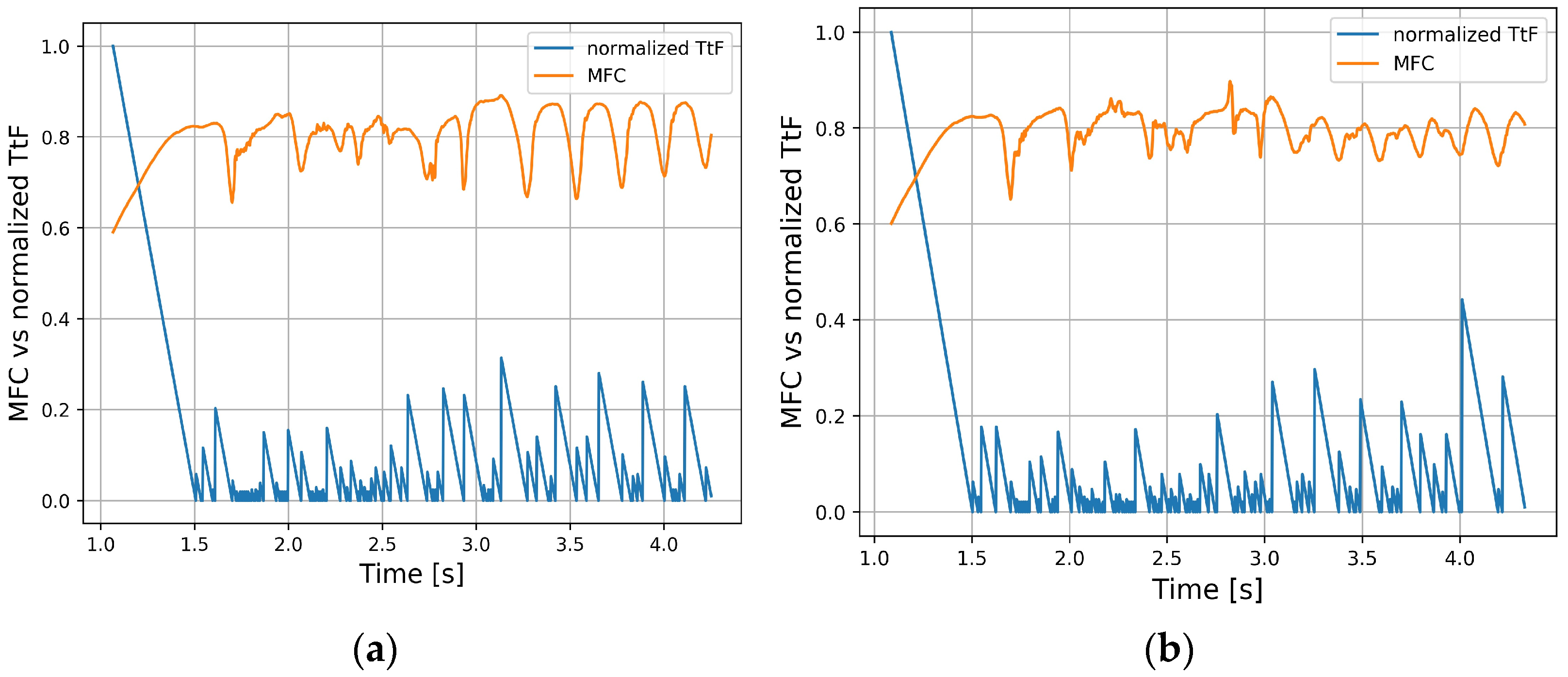
Figure 5 compares the MFC within the SI for each experiment with the TtF. The TtF values were normalized with respect to their maximum value to enable direct comparison with the MFC curves.

As shown in Figure 5, after the completion of each numerical earthquake, the TtF curve rises sharply to its maximum value and then gradually decreases as the end of the numerical event approaches.

3.6. Achievements of Machine Learning Algorithms

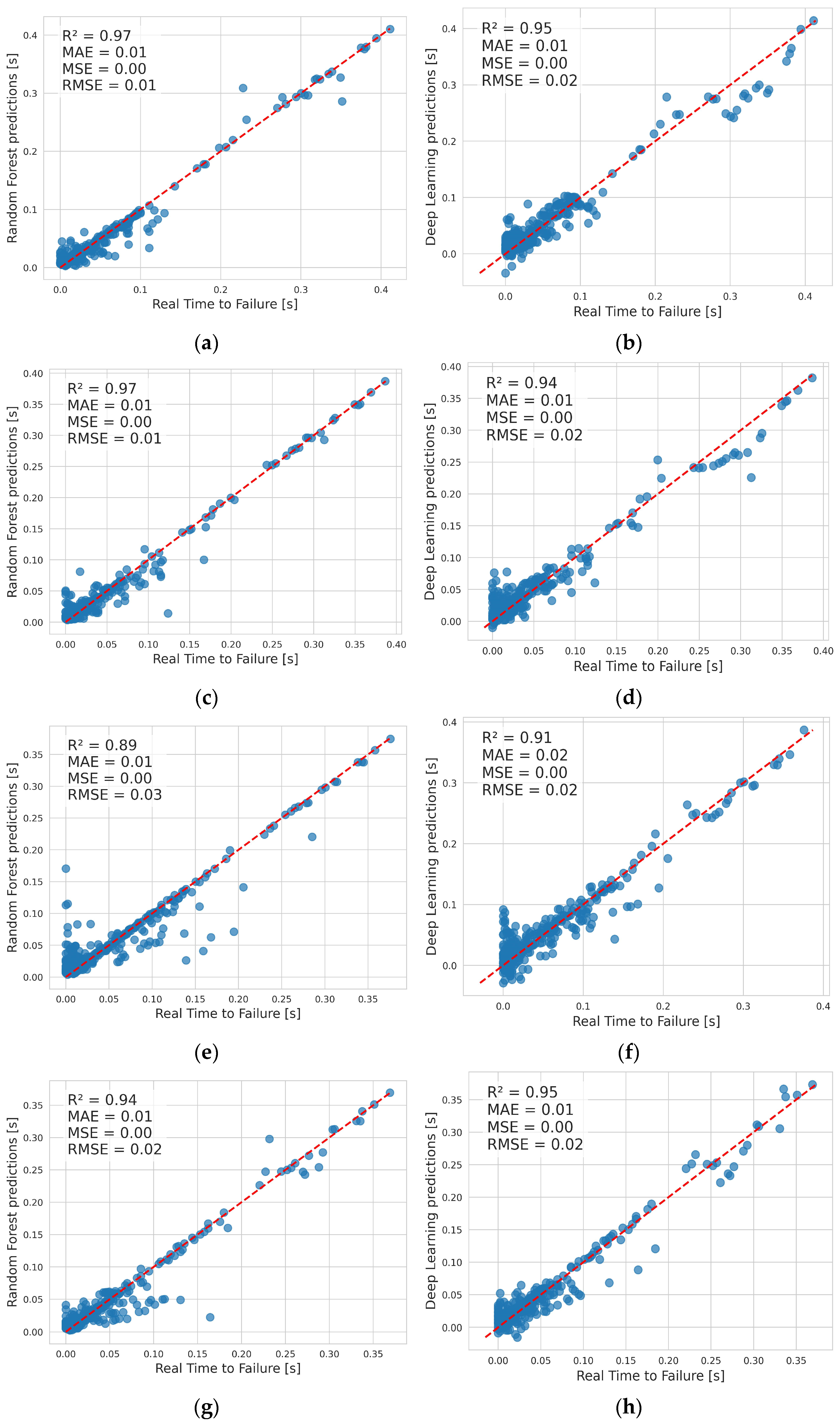
RF and DL performed very well with the predictions, as shown in

Table 2. Features used for Time to Failure prediction.

Experiment		Evaluation Metrics
		R2		MAE		MSE
		RF	DL	RF	DL	RF	DL
Training dataset	E1	0.9486 ± 0.0080	0.9238 ± 0.0143	0.0109 ± 0.0007	0.0174 ± 0.0022	0.0004 ± 0.0001	0.0006 ± 0.0001
	E2	0.9580 ± 0.0163	0.9333 ± 0.0082	0.0093 ± 0.00093	0.0159 ± 0.0025	0.0003 ± 0.0001	0.0005 ± 0.0001
	E3	0.8906 ± 0.0242	0.8608 ± 0.0203	0.0137 ± 0.0014	0.0204 ± 0.0009	0.0007 ± 0.0002	0.0009 ± 0.0001
	E4	0.9424 ± 0.0177	0.9359 ± 0.0105	0.0099 ± 0.0009	0.0143 ± 0.0013	0.0003 ± 0.0001	0.0004 ± 0.0001
Testing dataset	E1	0.9719	0.9434	0.0081	0.0137	0.0002	0.0004
	E2	0.9665	0.9572	0.008	0.0108	0.0002	0.0003
	E3	0.8858	0.8866	0.0132	0.0196	0.0007	0.0007
	E4	0.9432	0.9306	0.0094	0.0147	0.0003	0.0004

. Results are presented for the training and testing datasets for experiments E1–E4 for the R², MAE, and MSE metrics. Metrics on the training dataset are given as means with standard deviation, as they were the result of 5-Fold Cross Validation. Very good R² metrics above 90% were obtained. Experiment E3 was an exception, with a result below 90%. The MAE and MSE metrics had small values, indicating accurate predictions. Overall, RF performed slightly better than DL.

Figure 6 visually presents the predictions of the RF and DL algorithms on the test set. Ideally, all points would fall on the dashed straight line, indicating 100% prediction accuracy. It can be seen that the predictions are clustered close to the ideal prediction line, confirming the very good results of the metrics in Table 2.

The obtained results indicate that both machine learning algorithms, RF and DL, performed very well in predicting outcomes using only features derived from PAE. In most cases, the coefficient of determination (R²) exceeded 90% for both algorithms, on both the training and test datasets. However, in dynamical systems with strong temporal autocorrelation, such as numerical stick–slip cycles, random splitting leads to interpolation rather than true temporal prediction. In this case, neighboring time steps represent nearly identical physical states, which results in inflated performance metrics due to information leakage between the datasets. Therefore, the coefficients of determination reported in Table 2 should be treated as an upper estimate of model performance within a closed numerical system. The physical relevance of the method was evaluated using sequence-preserving predictions of complete data series, as presented in Section 3.9.

The DL model used in this study was a simple feed-forward Multi-Layer Perceptron operating on instantaneous tabular features describing the system state. The purpose of this comparison was not to evaluate DL architectures designed for time-series analysis, such as recurrent networks (LSTM, GRU) or one-dimensional convolutional networks (1D-CNN), which require access to the history of previous events. Instead, the Random Forest model was compared with a basic neural network capable of performing regression on individual data records. Therefore, the conclusion regarding the higher predictive performance and computational efficiency of the Random Forest model applies only to this comparison with a simple Multi-Layer Perceptron architecture and should not be generalized to DL methods as a class of temporal prediction models.

3.7. Computational Time—Training of RF and DL

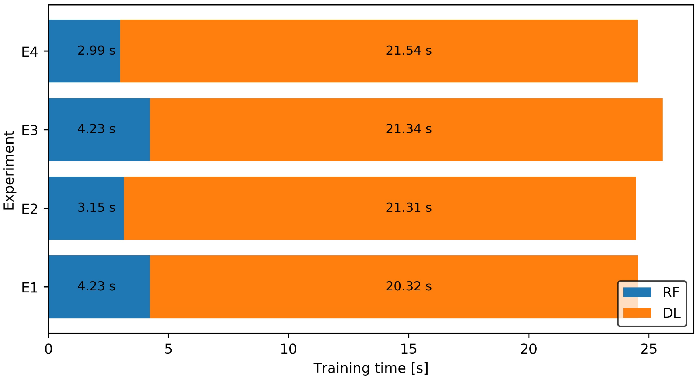
DL models are generally more expressive than classical supervised machine learning algorithms; however, they are often associated with higher computational cost. The actual training times of the RF and DL algorithms were compared (Figure 7). Training efficiency and computational time are important factors in determining which algorithm is more suitable for a given problem. For E1, the training time was 4.23 s for RF and 20.32 s for DL. For E2, the corresponding values were 3.15 s for RF and 21.31 s for DL; for E3, 4.23 s for RF and 21.34 s for DL; and for E4, 2.99 s for RF and 21.54 s for DL.

It was observed that the RF algorithm was approximately five to seven times faster than DL, and it achieved better metrics. In addition, a very simple DL architecture was used here, a more complex one would definitely be more time-consuming. This result indicated that DL was highly effective for analyzing large datasets with complex and nonlinear dependencies, but its application to other problems is computationally inefficient. In such cases, supervised machine learning algorithms are more appropriate.

3.8. In-Depth Analysis of the Impact of Features on Predictions with SHAP

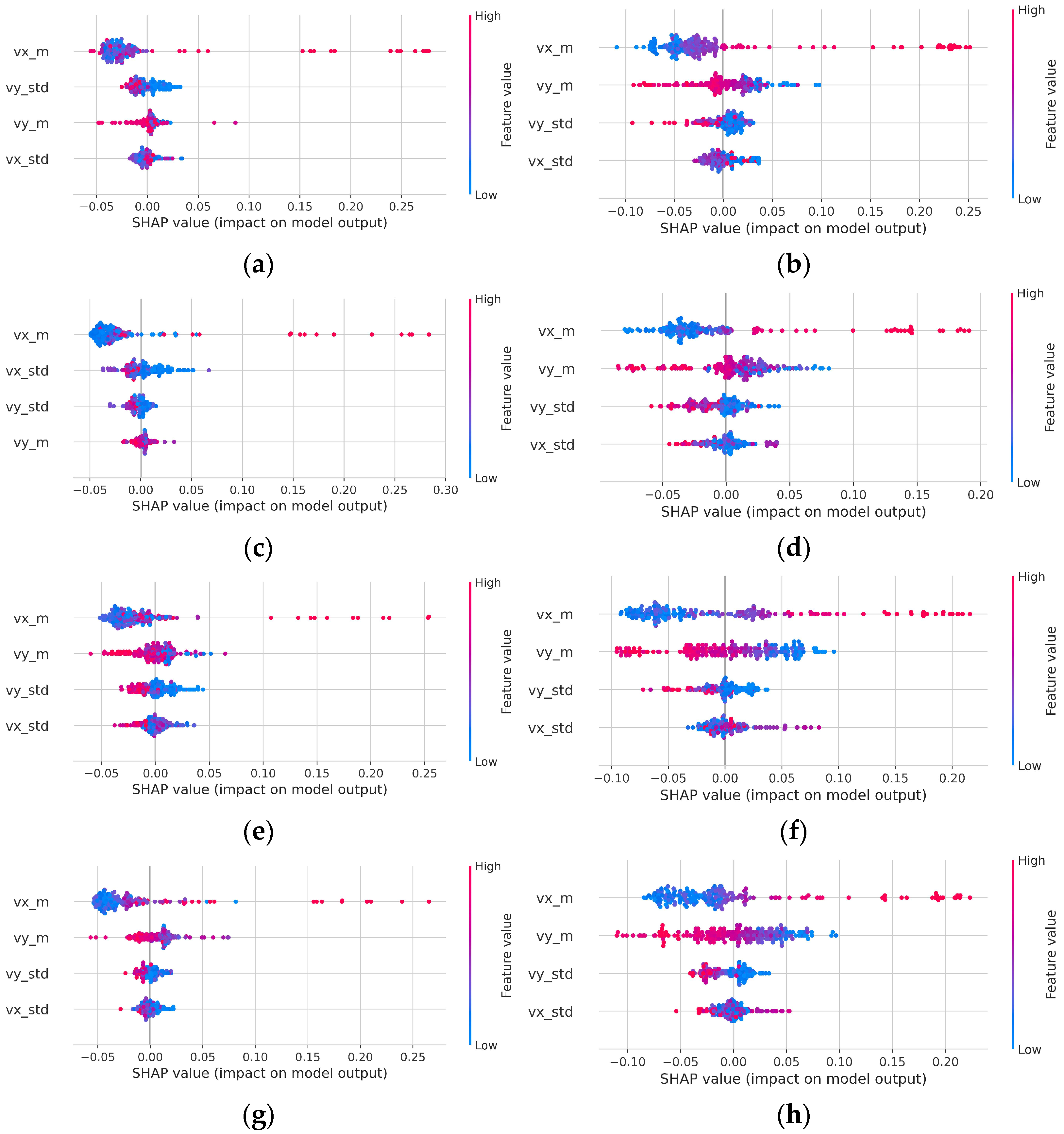
In the four configurations (E1–E4), a comparative analysis of the influence of features (independent parameters) was conducted for the RF and the DL using SHAP values (Figure 8). The order of parameters on the y-axis corresponds to their influence on the algorithm’s performance, ordered from highest to lowest. Across all experiments, the same pattern was observed—vx_m had the greatest impact on the performance of both the RF and DL models. In most cases, vx_std had the smallest impact. The second and third most influential parameters were the parameters related to velocity in the y-axis direction, i.e., vy_m and vy_std. Interestingly, this pattern was repeated for both the RF and DL models, despite the completely different characteristics of these models.

Regarding the x-axis of the SHAP plot, if the single data points had a high value (within a given feature), they were marked with a warm color. If they had a low value, then they were marked with a cool color. The position on the x-axis indicated the individual SHAP value calculated for each of the points. The results obtained in E1–E4 demonstrated high similarity, indicating that the observed dependency structure was not an artifact of a specific model architecture or data configuration. For both algorithms, low values of vx_m have a negative impact on model output, but data points are clustered close to the value 0. Conversely, high values of this feature have a high positive impact on model output, but data points are distributed irregularly along the axis. Regarding vy_m, the impact pattern is reversed compared with vx_m: high-value points have a strong negative impact, while low-value points have a strong positive impact. In the case of vx_std and vy_std, generally, small standard deviations give a low positive impact on model output, and high values of standard deviation give a low negative impact on model output.

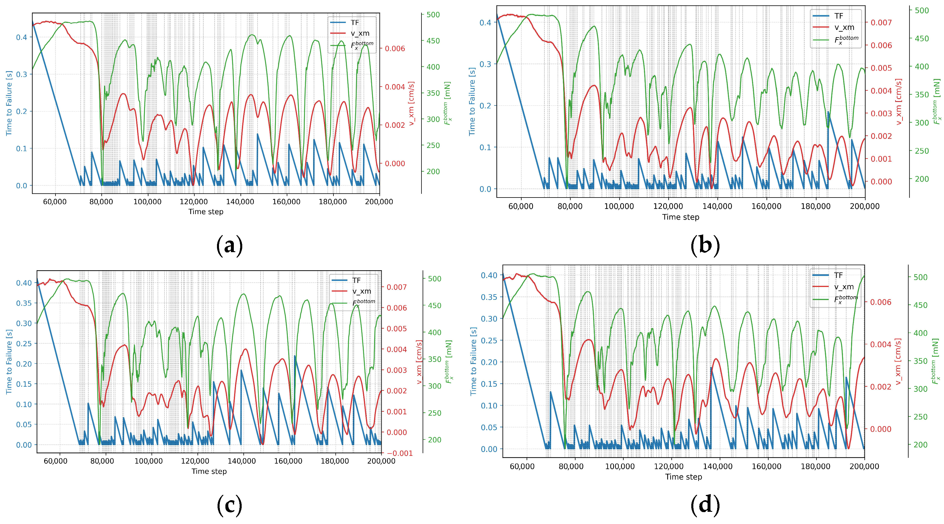
Using the most influential feature, vx_m, the precursory character of changes in vx_m relative to the TtF and the shear force acting on the bottom wall in the x-direction (Fx_bottom) was examined (Figure 9). In the applied DEM model the lower wall is driven at a constant velocity in the x-direction and is not subjected to a prescribed shear force. Consequently, the shear force acting on the bottom wall (Fx_bottom) is dynamically adjusted to maintain the imposed boundary velocity. The vx_m therefore reflects the internal dynamics of the granular medium, including local particle displacements, contact network rearrangements, and transient microslip processes, rather than the motion of the boundary.

A joint analysis of the temporal evolution of TtF, vx_m, and Fx_bottom (Figure 9) reveals no simple or monotonic relationship between these quantities. Elevated values of vx_m occur at different stages of the stick–slip cycle, both far from and close to the macroscopic stress drop, and local maxima of vx_m are not systematically synchronized with abrupt decreases in F_x_bottom or resets of TtF. Although changes in vx_m may precede the macroscopic force drop in some cases, they also frequently occur when the system remains far from global instability. Therefore, vx_m cannot be interpreted as a direct indicator of slip initiation or as a trivial detection of an ongoing event, but rather as a descriptor of the instantaneous dynamic state of the system.

Accordingly, the dominant contribution of vx_m identified by the SHAP analysis does not imply event detection, but indicates that this variable carries relevant, non-unique prognostic information that becomes meaningful only in combination with other input features. The machine learning model therefore uses vx_m as a key descriptor of the system’s progressive evolution toward a future macroscopic instability.

3.9. Predicting the Entire Numerical Earthquake

In the analyses presented above, the training of the RF and DL algorithms in experiments E1–E4 was based on a random selection of data points for the training and testing datasets. Although this is a standard procedure in machine learning, such an approach does not address whether the trained algorithm is capable of predicting an entire data sequence. In the context of numerical earthquake prediction, the primary objective is to forecast the TtF for an entire event. Therefore, a modified training approach was employed in the next stage of the study. Specifically, 90% of the initial TtF values in each experiment were used for training, while the remaining 10% of the final TtF values were reserved for testing. This approach enabled the algorithms to evaluate their predictive capability across the entire data series, effectively forecasting complete future events. 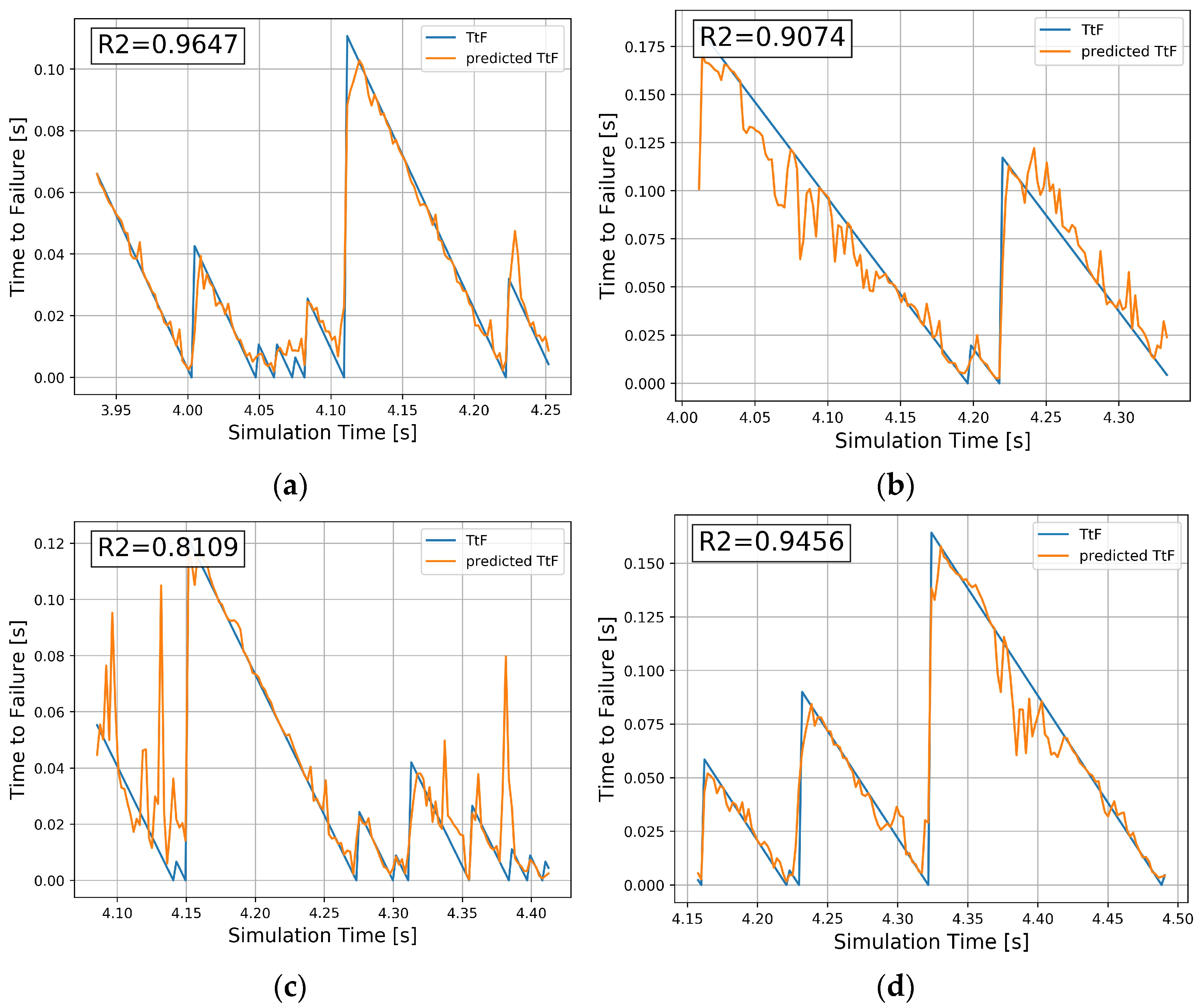Figure 10 presents a visualization of the prediction results for the last 10% of data points (testing dataset) from a representative segment of the curve. Only RF was used because it performed better for this type of problem than DL, as in Table 2.

The R² metric for each experiment was several percentage points lower than in Table 2, but overall, very satisfactory results were obtained. RF was able to predict and reproduce the TtF at every time step with satisfactory accuracy. Only in the case of E3 did intermittent predictions appear. These results demonstrated that RF was capable of predicting an entire series of events based on PAE monitoring.

4. Discussion

Scientific work is ongoing to better understand real seismic phenomena. However, at the current state of knowledge, the only earthquakes that can be predicted are those in the laboratory experiments [4,14] and those modeled numerically [8,13]. Machine learning helps in automatically finding patterns and relationships from huge datasets, especially nonlinear relationships. The methodology developed in this way can then be tested in the real world. This work is a continuation of scientific research in this area. A numerical DEM model reproducing stick–slip cycles was employed in this study. No formal modifications of the Discrete Element Method or new contact laws were introduced. The contribution instead concerned the use of DEM as an analytical framework for investigating frictional instabilities. In this approach, DEM was treated as a fully observable physical system in which the instantaneous microstate of the granular medium was related to the time remaining until the next slip event. Particle velocity statistics were interpreted as a numerical analogue of acoustic emission, accessible throughout the model volume. This allowed examination of the relationship between local contact reorganizations, kinematic fluctuations, and the progressive evolution toward instability, without reliance on the history of previous events. In this sense, the study extended the conventional application of DEM in stick–slip research.

The model used in this study was two-dimensional, representing a deliberate simplification relative to real three-dimensional granular media. The objective was not to directly simulate natural tectonic faults, but to analyze the dynamics of laboratory stick–slip friction systems, which were commonly investigated in quasi-two-dimensional experimental and numerical settings. In two-dimensional models, load transfer was restricted to a single plane, resulting in a more ordered force-chain topology and limited stress redistribution in the third dimension. As a consequence, force responses and macroscopic friction measures were more stable, allowing clearer identification of stick–slip cycles and their repeatable dynamic features. In three-dimensional or quasi-three-dimensional configurations, additional degrees of freedom permitted contact-network reorganization out of the shear plane, leading to more irregular force fluctuations and increased signal complexity at the boundaries. These differences mainly affected quantitative details and force-chain topology, whereas the fundamental dynamic mechanisms—such as stick–slip cyclicity, abrupt contact rearrangements, and the statistical character of events—remained qualitatively comparable between two- and three-dimensional systems. The main goal of this work, namely the development and testing of a time-to-failure prediction methodology based on instantaneous state descriptors, justified the use of a two-dimensional model. This approach reproduced key elements of laboratory seismic cycles while substantially reducing computational cost and data volume.

During the four numerical experiments, (pseudo) Acoustic Emission monitoring was carried out to estimate the time to subsequent numerical earthquakes. Quantities derived from mean particle velocities and their fluctuations were not interpreted as a direct equivalent of recorded acoustic emission signals, but rather as numerical descriptors of the intensity of dynamic processes acting as sources of wave emission. Under laboratory conditions, measured acoustic emission signals were further modified by wave propagation effects and boundary conditions, leading to filtering and spatial averaging of the source information. As a result, laboratory acoustic emission represented an integrated response of the medium, in which short-lived and spatially localized microslip activity resolved in the DEM model could be significantly attenuated or masked at the sensor scale. The term (pseudo) Acoustic Emission was therefore used to emphasize this distinction and to indicate that the analyzed quantities described the primary dynamic activity of the system rather than a direct measurement of acoustic waves. In future studies, this approach could be extended by incorporating virtual receivers and simplified wave propagation models, allowing a more direct comparison with laboratory acoustic emission experiments.

Two machine learning approaches—Random Forest and Deep Learning—were applied to identify relationships between the (pseudo) acoustic signal and the time to the next events. Only instantaneous values of parameters describing the system state were used as input variables, without incorporating delayed features or time-window statistics. This choice was deliberate and was based on the assumption that prediction of the time to the next event should rely on the current physical state of the system rather than on explicitly introduced historical information. This approach allowed a clear interpretation of the relationship between local grain dynamics and time to failure and enabled a distinction between state-based prediction and sequential modeling. The inclusion of delayed features or rolling statistics, which was common in classical time-series forecasting, represented a natural direction for future research but lay beyond the scope of the present work.

Main findings and conclusions of this work were as follows:

-

The present study was based on several simplifying assumptions; however, its objective was to provide a qualitative rather than a quantitative description of the investigated phenomenon.

-

High predictive performance was obtained on both the training and testing datasets using a random data split; however, this evaluation primarily reflected an interpolative setting and may have resulted in overestimated performance metrics due to temporal autocorrelation. Average coefficients of determination exceeded 0.95 on the training datasets and reached values above 0.97 on the testing datasets. Overall, the Random Forest model performed slightly better than the Deep Learning model.

-

Model training times were compared, showing that the Random Forest model required up to seven times less training time than the applied Deep Learning architecture, while achieving better evaluation metrics on both training and test datasets. This result highlighted the importance of comparing different machine learning approaches when selecting efficient predictive methods.

-

SHAP analysis of the input parameters showed that, among the four features constituting (pseudo) Acoustic Emission, the mean particle velocity in the x-direction had the strongest influence on model predictions for both Random Forest and Deep Learning.

-

As the main novelty of this study, it was demonstrated that the Random Forest algorithm was capable of predicting the time to failure for entire sequences of numerical earthquakes. Using only instantaneous particle velocity statistics and without relying on information about the history of previous events, coefficients of determination in the range R² = 0.81–0.96 were obtained.

-

The results confirmed that earthquake prediction is feasible in numerical and laboratory experiments using machine learning, where extensive information about the system state is available. In contrast, the limited availability of data in real-world seismic systems restricts the direct applicability of such approaches.

-

Scientific research under controlled conditions was therefore required to develop methodologies that could later be assessed with respect to real phenomena. For validation purposes, future studies could progressively transition from fully observable DEM models to data acquisition approaches representative of laboratory measurements. Within the same DEM framework, kinematic quantities would not be averaged over the entire system; instead, signals could be recorded by a network of virtual receivers located at the model boundaries. The resulting velocity or acceleration time series would be comparable to acoustic emission signals obtained in laboratory stick–slip experiments.