Article

Multi-Objective Optimization Based on Kriging Surrogate Model and Genetic Algorithm for Stiffened Panel Collapse Assessment

by
João Paulo Silva Lima
1,
Raí Lima Vieira
2,
Elizaldo Domingues dos Santos
2,
Luiz Alberto Oliveira Rocha
2,* and
Liércio André Isoldi
2
1
Faculty of Science and Technology, Federal University of Goias (UFG), Aparecida de Goiânia 74968-755, Brazil
2
Graduate Program in Ocean Engineering (PPGEO), School of Engineering, Federal University of Rio Grande (FURG), Rio Grande 96203-900, Brazil
*
Author to whom correspondence should be addressed.
Appl. Mech. 2025, 6(2), 34; https://doi.org/10.3390/applmech6020034
Submission received: 20 February 2025 / Revised: 15 April 2025 / Accepted: 28 April 2025 / Published: 30 April 2025

Abstract

:
A hyperparameter-optimized Kriging surrogate model was developed for the structural collapse behavior framework presented in this paper. The assessment is conducted on a stiffened panel subject to axial load and lateral pressure, typical of the deck structure of a bulk carrier ship. This behavior is characterized using nonlinear finite element analysis to determine the collapse response. The surrogate model’s hyperparameters were optimized using a Genetic Algorithm to achieve the best performance, and the trained framework can predict ultimate strength. By following this approach, the problem can be reformulated as a multi-objective optimization task. This framework involves associating the Kriging surrogate model with a multi-objective evolutionary optimization algorithm based on Genetic Algorithms to balance the trade-off between the weight and ultimate strength of the stiffened panel. The results confirm the applicability of the Kriging surrogate framework to predict the ultimate strength and assess the collapse analysis of the stiffened panels, ensuring accuracy through GA-based hyperparameter optimization.

1. Introduction

The integrity of a ship’s structure needs to be increased to ensure the safety of bulk carriers. A ship’s structure relies on stiffened panels as essential components to withstand the external longitudinal bending moments created by the buoyancy, wave forces and moments, and cargo weight distribution.
In extreme sea conditions, the most perilous scenario occurs when the wavelength matches the ship’s overall length, resulting in maximum bending moments. Bending moments can surpass the load-carrying capacity limit in such cases, leading to severe tensile and compressive loads on the deck and bottom-stiffened panels. Consequently, the local structures of the deck and bottom experience post-buckling and collapse due to their distance from the neutral axis of the cross-section [1,2]. Investigating the collapse behavior of the ship’s bottom under axial load conditions associated with lateral pressure can significantly improve ships’ economical and safe design, allowing a promising future for ship design.
Many research studies have been conducted to better understand the plastic collapse behavior and strength of structural components, particularly through developing novel methodologies for predicting their ultimate strength under various loads. Wang and Moan [3] examined collapse behaviors by analyzing the ultimate strength of stiffened panels under biaxial and lateral loading to assess the beam-column approach used in regulations for ships and offshore structures. Guedes Soares and Gordo [4] derived equations to assess the strength of plates subject to biaxial compressive loads, including the effect of initial distortions and residual stresses. Fujikubo et al. [5] proposed a formula to estimate the ultimate strength of steel stiffened panels subjected to combined transverse compression and lateral pressure, highlighting the interaction influence of adjacent plates and stiffeners. Benson et al. [6] introduced an adapted large deflection orthotropic plate methodology to analyze local and overall panel collapse modes. Li et al. [7] developed an analytical method to predict plate and stiffened panels’ buckling and collapse behavior under cyclic loading.
Undoubtedly, the Finite Element Method (FEM) has a wide application in the post-buckling behavior analyses of stiffened panels. Most numerical studies were performed on the ultimate strength of stiffened panels under axial loads and lateral pressure [1,5,8,9,10,11]. However, FE software for addressing complex nonlinear problems continues to pose challenges in the design practices of the naval industry. This is primarily because the results of FEA are susceptible to the input parameters and the solution algorithms utilized [12]. The ISSC 2022 Committee III.1 on Ultimate Strength highlights those uncertainties related to material modeling, geometric imperfections, and human factors in the analysis that can significantly impact the accuracy of FEA results [13].
Beyond that, the collapse behavior in marine structures is enhanced and understood by taking into account the investigations about slenderness [9,14,15], boundary condition [8,16], initial imperfection [4,17,18,19], openings [20,21], corrosion [22,23,24], and cracks [11,25,26]. Additionally, given the complexity of developing FE models, it is crucial to carefully select mesh sizes and boundary conditions to achieve accurate and reliable results [11]. However, a balance must be ensured between computational accuracy and cost.
On the other hand, surrogates have been widely applied in designs to replace expensive physical experiments or time-consuming simulations. To replace structural numeral simulations, they are constructed based on limited finite element calculations reducing the computational burden and providing predictions based on the fitted or interpolated mathematical relationships. Initial efforts are proposed using polynomial regression models [27,28] and are currently used in prediction problems (e.g., [29,30,31]). Other approaches adopted the Support Vector Machine (SVM) Model (e.g., [32,33]), Polynomial Chaos Expansion Models (e.g., [34,35,36]), Gaussian Processes (e.g., [37,38,39]), and Artificial Neural Networks (ANNs) (e.g., [40,41,42,43]). Instead of polynomial fits, approaches based on the Kriging surrogate model have been proposed [44,45,46,47].
The Kriging surrogate model offers several evident benefits. Notably, it can effectively capture hidden relationships in high-dimensional parameter spaces using observed data, making it particularly suitable for small datasets [48]. Additionally, the Kriging surrogate provides robust uncertainty estimations, enabling the exact inference for the observed dataset with zero variance while also predicting alongside a mean prediction amongst unknown observations [48,49,50]. In contrast, many other surrogate models, such as polynomial regression, ANN, SVM, and Radial Basis Functions (RBFs), are regression-based and can even produce accurate predictions with errors even at training points.
Given these considerations, Kriging offers strong interpretability, making it a more promising modeling and optimization design option [50]. Due to its advantages, Kriging has been successfully utilized as the surrogate model in numerous research projects in the naval industry. As a surrogate solution, instead of polynomial fits, approaches based on the Kriging surrogate model have been proposed [51,52]. In a structural collapse behavior assessment, Gaspar et al. [44] studied Kriging’s efficiency for double-hull oil tanker ship stiffened panels’ reliability analysis. In Shi et al. [53], the prediction accuracy of the Kriging model is assessed to estimate the failure probability of marine structures with its application to a stiffened panel. Lima et al. [54] assessed the reliability behavior of stiffened panels of ship hulls using a Kriging multi-fidelity surrogate, which uses the finite element analysis (FEA) to obtain the high and low-fidelity dataset.
Considering a structure’s post-buckling ultimate load capacity, it becomes possible to design more efficient structures that can reduce overall weight [55,56]. The weight of a vessel’s hull is a crucial design parameter that impacts the entire performance of a ship. It relates to functional requirements, construction costs, operational expenses, maintenance, and durability. Therefore, selecting an optimal structure is essential for achieving the best structural performance [57]. Consequently, it is essential to design the structural members optimally, using the optimal geometric dimensions for the plates and ensuring proper geometric relationships for the stiffeners applied.
Surrogate models utilize implicit knowledge within the design problem to enable rapid evolution, comprehensive approximate modeling, and optimization while minimizing the number of costly simulations required. As a result, these models enhance optimization efficiency and convergence accuracy, significantly reducing the time consumed [49].
Accordingly, the present paper aims to propose a surrogate-assisted evolutionary algorithm to solve a multi-objective optimization problem (MOP), considering the weight vs. ultimate strength of bulk carrier stiffened panels for structural post-buckling analysis. The main contribution is developing a hyperparameter-optimized Kriging surrogate model, considering the advantages of a Genetic Algorithm, focusing on prediction accuracy, stability, and computation efficiency applied in a typical marine industry issue. As a numerical framework, a stiffened panel under axial load and lateral pressure typical of the deck structure of bulk carrier model ships is adopted and described using nonlinear FEA to obtain the collapse behavior. The Kriging surrogate model is used to predict the ultimate strength, and the Non-Sorting Genetic Algorithm (NSGA-II) is used to perform multi-objective optimization.
This paper is organized as follows: Section 2 introduces the real application problem, considering a numerical example, and the FEA model for the present research. Section 3 presents the Genetic Algorithm multi-objective optimization based on the Kriging surrogate model. In Section 4, this study’s results are discussed extensively. Section 5 draws the main conclusions of the work conducted.

2. Ultimate Strength of Stiffened Panel Under Combined Loading

The stiffened panel is a fundamental structural element in shipbuilding, and extensive research has been conducted over the past few decades. These studies examine the effects of initial deflections, boundary conditions, and residual stresses on the ultimate strength (σzu) of the panel. Additionally, the applied loads can vary, ranging from axial and biaxial loading to lateral pressure. This section presents the structural model of the stiffened panels of the bulk carrier ship’s bottom under a combined loading considering axial compression associated with lateral pressure and describes the finite element model used for its reproduction and structural analysis.

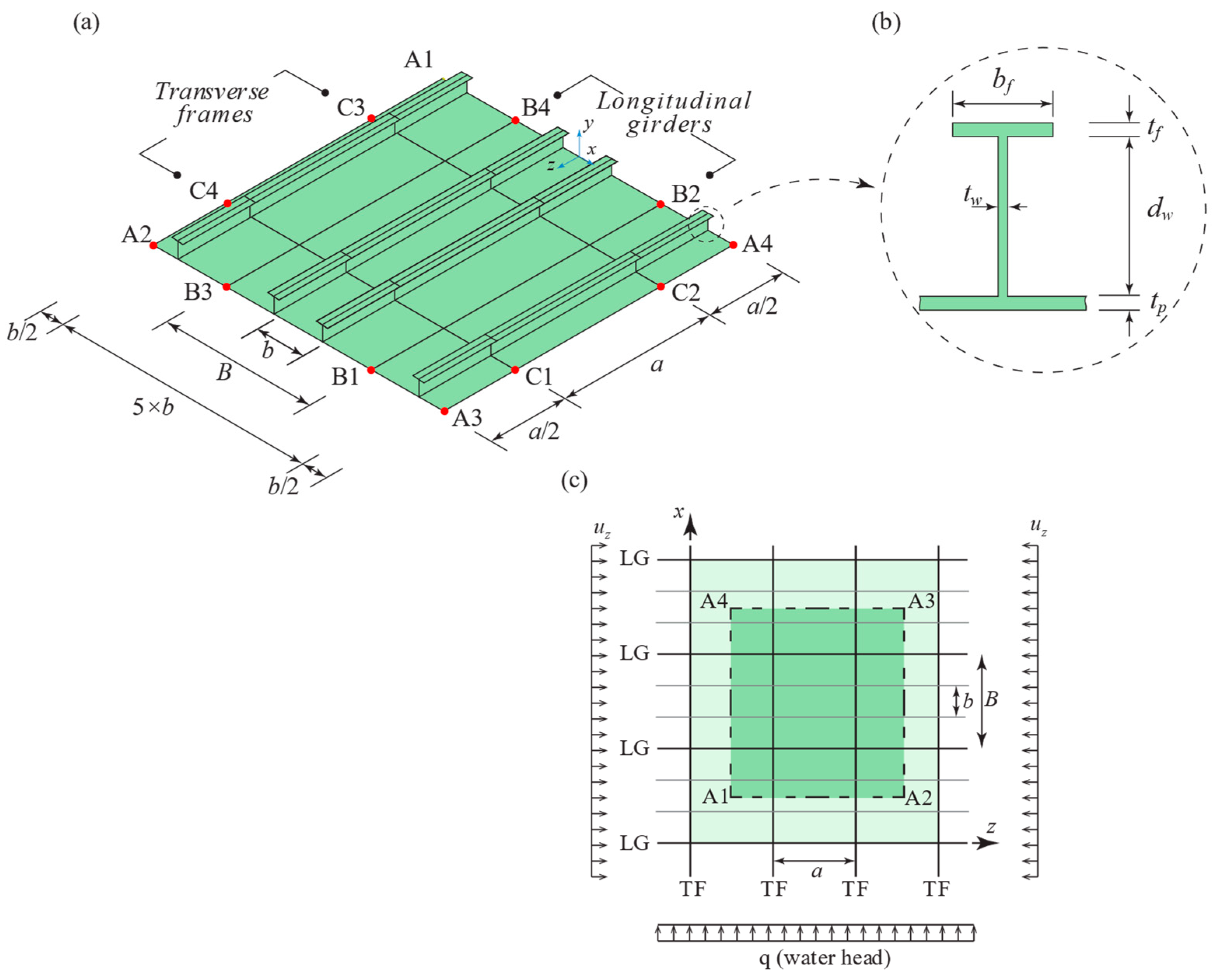
2.1. Case Study: Bulk Carrier Stiffened Panels

The dimensions of the stiffened panels are based on the benchmarks established in the ISSC 2012 Committee III.1 [58], taking into account the members of the actual ship. For the benchmark analysis, fundamental models were selected, specifically, stiffened panels from the bottom plating of a bulk carrier. These panels feature two stiffeners and are subjected simultaneously to lateral pressure and in-panel compression. This framework was previously adopted in the studies conducted by Tanaka et al. [9] and Xu et al. [8].
For this study, the local panel has an aspect ratio of a/b = 3 (a × b = 2550 × 850 mm). This panel is part of a stiffened structure, which is divided by longitudinal girders (LGs) and transverse frames (TFs), as illustrated in Figure 1a. Consequently, the chosen type of stiffener is the ‘Tee-Bar’. The referenced values in [58] are associated with Tanaka et al. [9] and Xu et al. [8] to determine the variable ranges in the present study. Figure 1b displays the geometries of the stiffeners, and Table 1 offers a detailed overview of the various stiffened plate parameters.
The material is assumed to be elastic and perfectly plastic. The steel assumed in the analyses have a Yield stress of σY = 313.6 MPa, Young’s modulus of E = 205.8 GPa, Poisson’s ratio of υ = 0.3, and strain hardening rate: H’ = 0.

2.2. Geometrical Initial Imperfections

The initial imperfections in stiffened plates arise from the unavoidable deformations that occur during the complex fabrication and welding processes of the ship’s steel structure [59,60]. The σzu behavior of a plate subjected to buckling loads varies significantly based on the shape of the initial deflection [61]. A portable 3D scanner can be used to measure initial imperfections before experiments and be adopted in analyzing the nonlinear buckling behaviors in FE simulations [19]. However, accurately modeling the realistic distributions of initial spatial deformations in stiffened panels is challenging due to their complexity, making them difficult to replicate in FE analysis [2].
The shape of welding-induced initial deflections for thin plates after support members are attached by welding in real ship hull analysis is quite complex. However, the actual level of model initial imperfections can be simplified by a method of analysis that assumes the same shape as the Fourier components [5]. In the present study, the following three types of deflections are assumed to be the initial imperfections of the stiffened panel [2,8,9,14,62]:
  • Initial deflection of local plate panel (Figure 2a):
    w 0 p = A 0 sin m π z a sin π x b + B 0 sin π z a sin π x B
  • Column-type deflection of stiffeners (Figure 2b):
    w 0 c = B 0 sin π z a sin π x B
  • Side-way deflection of stiffeners due to angular rotation around panel stiffener (Figure 2c):
w 0 s = C 0 x d w sin π z a
where a and b are the length and width of local rectangular plates, B is the width of the stiffened panels between girders, and A0 = 0.1β2tp and B0 = C0 = 0.0015a are the following design values for the amplitudes. The number of buckling half-waves in the longitudinal direction (m) is normally the integer of the ratio of the longer and shorter side of the plate m = a/b and is considered m = 6. The plate slenderness β is defined as follows:
β = b t p σ y E
The plate deflections are considered periodical in the local and overall buckling modes due to the continuous property of the intact stiffened panel [8,9,10]. Additionally, the stiffened plate is selected as a (1/2 + 1 + 1/2) span, and the (1/2 + 1 + 1/2) bay model with periodical boundary condition is adopted considering the interaction between the adjacent stiffeners and plate influence [8], as shown in Figure 2d.
To accurately evaluate σzu, the model used must sufficiently represent the surrounding structure of the given panel. In Figure 1, the notations x, y, and z refer to the transverse, lateral, and longitudinal directions, respectively. The boundary conditions are defined as follows: ux, uy, and uz represent the translational displacements in x, y, and z directions; and θx, θy, and θz indicate the rotational displacements around x, y, and z directions. The current analysis considers the following boundary conditions, where “0” signifies a constraint and “1” no constraint:
  • A1A4 border: u x = u x * ,    u y = u y * ,    u z = d z ,    θ x = θ x * ,    θ y = 0 ,    θ z = θ z * ;
  • A2A3 border: u x = u x * ,    u y = u y * ,    u z = 0 ,    θ x = θ x * ,    θ y = 0 ,    θ z = θ z * ;
  • A1A2 and A3A4 border: u x = 0 ,    u y = 1 ,    u z = 1 ,    θ x = 1 ,    θ y = 0 ,    θ z = 0 ;
  • C1C4 and C2C3 for plate nodes: u x = 1 ,    u y = 0 ,    u z = 1 ,    θ x = 1 ,    θ y = 0 ,    θ z = 0 ;
  • C1C4 and C2C3 for stiffener web: u x = 0 ,    u y = 1 ,    u z = 1 ,    θ x = 1 ,    θ y = 0 ,    θ z = 0 ;
  • B1B2 and B3B4: u x = 1 ,    u y = 0 ,    u z = 1 ,    θ x = 0 ,    θ y = 0 ,    θ z = 1 ;
where dz indicates the uniform displacement imposed at the transverse edge, and (*) signifies that the displacement components are the same at the two nodes located opposite each other at the two opposite edges. The plate’s lateral pressure q models the water pressure, and the behavior of the stiffened panel under lateral loads is assessed by varying the load q between 0 and 0.3 MPa.

2.3. The FE Description

The post-buckling behavior of the stiffened panel under uniaxial compression is obtained using the FE software ABAQUS v.14. The finite element S4R available in the ABAQUS FE code are used to obtain the nonlinear structural behavior of the stiffened plate elements under combined loading. The S4R element is a four-node general-purpose quadrilateral shell element that utilizes reduced integration and accommodates large-strain formulation in ABAQUS.
To ensure accurate and valid results, it is essential to explore and refine the mesh. However, it is also important to strike a balance between the required precision and the computational effort to optimize computing time. Based on the convergence study for an intact stiffened panel, we established that the element size of the mesh should be set at 50 mm. The initial deflections are introduced to the mesh by adjusting the coordinates of the model nodes according to Equations (1)–(3), resulting in a modified mesh.
The lateral pressure and the in-plane forces are applied in two steps. First, the pressure is applied in the lateral direction of the plate, followed by the forced displacement applied along the edge of the stiffened panel [8].

3. Genetic Algorithm Multi-Objective Optimization Using Kriging Surrogate

This section outlines the computational framework of a Multi-objective Evolutionary Algorithm (MOEA) based on a Genetic Algorithm (GA). A Kriging surrogate model assists the multi-objective optimization in predicting the ultimate strength of stiffened panels under combined loading.

3.1. Structural Collapse Assessment Using GA-MOEA Kriging Surrogate Model

The GA-MOEA Kriging framework is illustrated in the flowchart in Figure 3. In Stage 01, the Kriging surrogate model is developed and optimized for hyperparameters. In Stage 02, this surrogate model is integrated into the evolutionary multi-objective optimization process. The detailed steps of the proposed algorithm are given as follows:
Stage 01—Step 1: An initial random dataset is used to create the surrogate model. This dataset consists of n train observed data X 0 = x 1 , x 2 , , x n t r a i n T , each with corresponding responses Y 0 = y 1 , y 2 , , y n t r a i n T  that build the initial dataset input D train = X 0 , Y 0 used to estimate the Kriging hyperparameters. To evaluate the performance of the final hyperparameter-optimized surrogate model, the dataset D test = X t e s t , Y t e s t is used, considering X t e s t = x t e s t ( 1 ) , x t e s t ( 2 ) , , x t e s t n t e s t T and Y t e s t = y t e s t 1 , y t e s t 1 , , y t e s t n test T with a total of n t e s t observed data, never seen during training. The database is generated randomly by Latin Hypercube Sampling. The maximin criterion is utilized in sampling to effectively fill the design space and assess the uniformity of the sampling plan. This approach aims to maximize the minimum Euclidean distance between sample points in a Latin hypercube. For those interested in more details about generating the optimal Latin Hypercube Sampling, please refer to the study of [63].
Stage 01—Step 2: In parallel computing, the output Y ˜ = Y 0 ; Y t e s t is obtained by nonlinear FEA. In this step, a computational analysis is conducted to predict the ultimate strength of each stiffened panel in the dataset.
Stage 01—Step 3: A hyperparameter optimization based on the GA is proposed to obtain the best performance of the Kriging surrogate model. This step maximizes the likelihood of the data field, obtaining the Maximum Likelihood Estimation. After the model is built, the accuracy of the test data prediction set is calculated.
Stage 01—Step 4: Steps 2 and 3, along with the corresponding hyperparameter optimization, are repeated until the convergence criteria are met. To quantify the accuracy of the proposed Kriging surrogate model, the mean relative error (MRE), considering the sum of relative errors divided by the sample size, is given as follows:
MRE = 1 n t e s t i = 1 n t e s t y ^ t e s t ( i ) y t e s t ( i ) y t e s t ( i ) ,
where y ^ t e s t denotes the output of the Kriging surrogate prediction. It is considered MREstop = 1%.
Stage 02—Step 1: The optimal solutions of the Pareto front are obtained using the Non-Sorting Genetic Algorithm, a multi-objective evolutionary optimization method. The multi-objective problem can be formulated as the following constrained optimization problem:
minimize    F ( x ) = ( F 1 ( x ) , F 2 ( x ) ) T subject   to    q q r e f
where F(x) represents two objective functions. The first, F1(x), signifies the mass of the stiffened panel, while the second, F2(x), represents the ultimate strength of the stiffened panel. The negative sign is used to indicate a maximization of the function. Additionally, g(x) denotes an inequality constraint related to the lateral pressure (q) which is limited to a specific reference value, denoted as qref.

3.2. Kriging Surrogate Model

The Kriging model is introduced in the geostatistics by Krige in 1951 [64]. It is an interpolation-based surrogate model that approximates the input/output function f. The Kriging surrogate model is assumed in a non-parametric probabilistic model to predict response values at unknown points based on a set of sample input data X0 and the observed values Y0. According to Forrester and Sóbester [65], considering x, the design variables in a Dk dimension and the formulation of the Kriging can be presented as follows:
f ^ x = G x T η + Z x
where f ^ x is the Kriging approximation, G x T is the basis function vector, η is the unknown regression coefficients of the trend function, and Z is the stationary Gaussian process error model, which has zero uncertainty at the training points. The covariance matrix Z is modeled using the correlation matrix:
cov Z x i , Z x j = σ 2 ψ x i , x j
where σ2 is the variance, and ψ(·) are correlations between a random variable at the point to be predicted and at the sample data points:
ψ x i , x j = exp k = 1 n v θ ^ k x k i x k j p ^ k
where nv is the number of design variables and θ ^ , p ^ k are spatially related parameters. From this, an n × n correlation matrix of all the observed data is constructed:
Ψ = ψ x 1 , x 1 ψ x 1 , x n ψ x n , x 1 ψ x n , x n .
The covariance matrix based on the Kriging model is then as follows:
cov y x , y x = σ 2 Ψ
To determine the correlations used in the correlation matrices, it is necessary to estimate the hyperparameters θ ^ . According to the Maximum Likelihood Estimation (MLE) theory, an optimization in unconstrained scenario is utilized to obtain the following:
MLE = n 2 ln 2 π n 2 ln σ 2 1 2 ln det Ψ y 1 μ T Ψ 1 y 1 μ 2 σ 2
Derivate Equation (12) into μ concerning and σ2 to 0, and find MLEs of the following:
μ ^ = 1 T Ψ 1 y / 1 T Ψ 1 1 ,    and
σ ^ 2 = y 1 μ ^ T Ψ 1 y 1 μ ^ / n
Substituting Equations (13) and (14) back into ln-likelihood yields the concentrated ln-likelihood function:
MLE = n 2 ln σ ^ 2 1 2 ln det Ψ .
The hyperparameters θ ^ are obtained by maximizing Equation (15). Since the hyperparameters cannot be obtained theoretically, they can only be obtained by the numerical maximization of Equation (15). It is assumed that p ^ k = 2 rather than using an MLE. The Genetic Algorithm (GA) optimization [65] is adopted to estimate the hyperparameters and maximize the MLE.
To predict an unknown y ^ at x * should be consistent with the observed data and the correlation parameters. The new prediction is combined with the existing data, to create the vector y ˜ = y T , y ^ T . The correlation defines the relationship between the observed data and the new prediction:
ψ = ψ x 1 , x * ψ x n , x * .
The augmented covariance matrix is as follows:
Ψ ˜ = Ψ ψ ψ T 1 .
To maximize MLE y ^ x n + 1 , it is necessary to maximize:
MLE = y ˜ 1 μ T Ψ ˜ 1 y ˜ 1 μ ^ 2 σ ^ 2 ,
which may be expressed as
MLE = y 1 μ ^ y ^ μ ^ T Ψ ψ ψ T 1 1 y 1 μ ^ y ^ μ ^ 2 σ ^ 2 .
Calculating the inverse of Ψ ˜ , the maximum of the quadratic function of y ^ is obtained by differentiating with respect to y ^ and setting to zero:
1 σ ^ 2 1 ψ T Ψ 1 ψ y ^ μ ^ + ψ T Ψ 1 y 1 μ ^ σ ^ 2 1 ψ T Ψ 1 ψ = 0 .
Finally, the MLE for y ^ is as follows:
y ^ x * = μ ^ + ψ T Ψ 1 y ^ 1 μ ^ .

3.3. Genetic Algorithm Optimization

The Genetic Algorithm (GA) was selected as the optimization method for this study because of its widespread use in optimizing hyperparameters of surrogate models. The GA process consists of several key steps: initializing a population, selecting the fittest individuals, applying natural processes such as crossover and mutation, and reproducing the population. This subsection provides a brief overview of the four steps of GA, with additional details available in references [66,67].
Step 1: A random population is initialized, and each member of the current population is scored by computing its fitness value. These values are called the basic fitness scores.
Step 2: The algorithm identifies suitable members, referred to as parents, based on their fitness values. These parent individuals mate to produce a new population. The selection function, Stochastic Uniform, arranges a line where each parent corresponds to a segment of the line that is proportional to its scaled value. The algorithm then moves along this line in equal-sized steps. At each step, it selects a parent from the segment where it lands.
Step 3: Three types of children are produced for the next generation: The first type consists of individuals from the current population with better fitness values, known as elites, who are carried over to the next generation. The second type is created through crossover, where the genetic information of two randomly selected parents is combined to produce offspring. Additionally, mutated offspring are generated by making random changes to the genetic material of one parent. The mutation offspring is created using Gaussian Mutation, which involves adding a random number selected from a Gaussian distribution to each entry of the parent vector. Typically, the degree of mutation, proportional to the standard deviation of the distribution, decreases with each new generation.
Step 4: The current population is replaced with children to form the next generation. This process helps prevent the GA from converging to a local optimum solution.
Step 5: The iteration concludes when either the convergence criteria are met, or the maximum number of evaluations is exceeded. If neither condition is satisfied, Step 2 is repeated.

3.4. Multi-Objective Optimization Problem Genetic Algorithm

This study utilizes a Genetic Algorithm Approach to Surrogate-Assisted Multi-objective Evolutionary Optimization Algorithm (GA-MOEA). An efficient MOEA is essential for generating solutions that closely align with the Pareto optimal front while ensuring that their distribution is both diverse and uniform within the resulting non-dominated front, all at a minimal computational cost.
In a typical multi-objective optimization problem with the vector of design variables x in the box constraints x _ and x ¯ , the goal is to minimize a set of p objective functions f i x , (i = 1, …, p) subject to q number of constraints g j x 0 , (j = 1, …, q). The previous can be summarized as follows:
Minimize [ f 1 x , f 2 x , , f p x ] Subject to g j x 0 ( j = 1 , , q ) x _ x x ¯ where x = ( x 1 , x 2 , , x l )
The Non-Sorting Genetic Algorithm II (NSGA-II) initially proposed by Deb et al. [68] has demonstrated its effectiveness in multi-objective optimization. Most terminology associated with the NSGA-II algorithm aligns with that of the GA discussed in Section 3.3. However, this section introduces additional terms specific to NSGA-II. In this study, NSGA-II is employed to identify the Pareto optimal design, following the steps outlined in the studies of [68,69,70,71,72].
This approach iteratively searches for non-dominated solutions across different fronts. First, for each solution i in the population, the algorithm calculates two key metrics: ni, which represents the number of solutions that dominate i, and Si, which is a set of solutions that i dominates, for which ni = 0 are classified into the first front. Next, for each member j in the set Si, the nj value is decreased by one. If any nj is reduced to zero during this stage, the corresponding member j is then assigned to the second front. This process continues for each member in the second front to identify the third front, and so forth.
Furthermore, NSGA-II applies the concept of crowding distance, where the crowding-distance value (CDi) of the ith solution is calculated as follows:
C D i = p = 1 k f p i + 1 f p i 1 f p m a x f p m i n
where f p i + 1 and f p i 1 denote the pth objective function of the (i + 1)-th and (i − 1)-th individual, respectively, and f p m a x and f p m i n represent the maximum and minimum values of the pth objective function. The primary process of the NSGA-II is as follows:
Step 1: An initial population is generated. The objective functions and constraints for this population are evaluated, and these values are used to calculate scores for the individuals within the population.
Step 2: The next generation’s parents are selected using the binary tournament selection method applied to the current population.
Step 3: Children are created from the selected parents through mutation and crossover. These children’s objective function values and feasibility are then assessed to obtain their scores.
Step 4: The current population is combined with the children to form an extended population. The rank and crowding distance for all individuals in the extended population are calculated. The crowding distance is a measure of the closeness of an individual to its nearest neighbors as a sum over the dimensions of the normalized absolute distances between the individual’s sorted neighbors.
Step 5: The extended population is pruned by retaining the appropriate number of individuals from each rank.
Step 6: The iteration concludes when the convergence criteria are met or when the maximum number of evaluations is exceeded. If neither condition is satisfied, Step 2 is repeated.

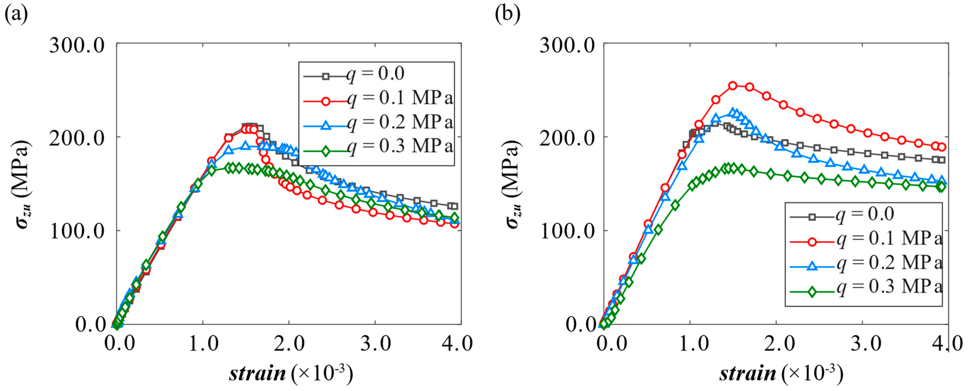
4. Analysis of Results

The databases of numerical analysis are required to derive a Kriging surrogate model for assessing the collapse behavior of stiffened panels and estimate the σzu behavior for each sample x(i). Moreover, the σzu behavior of the bottom-stiffened panel is defined by the stress–strain curves of the stiffened panels. The stress is defined as the applied force divided by the total area of the stiffener and plate.

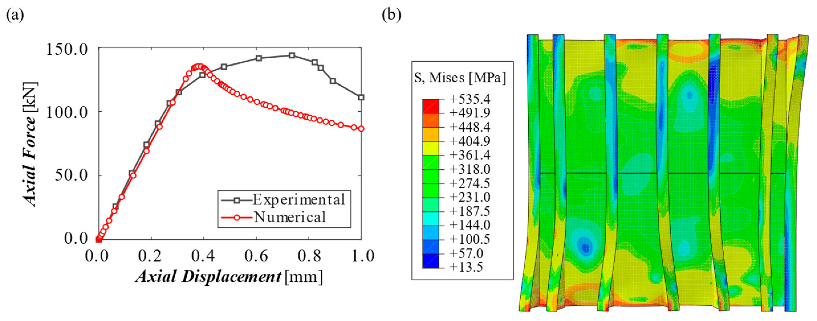
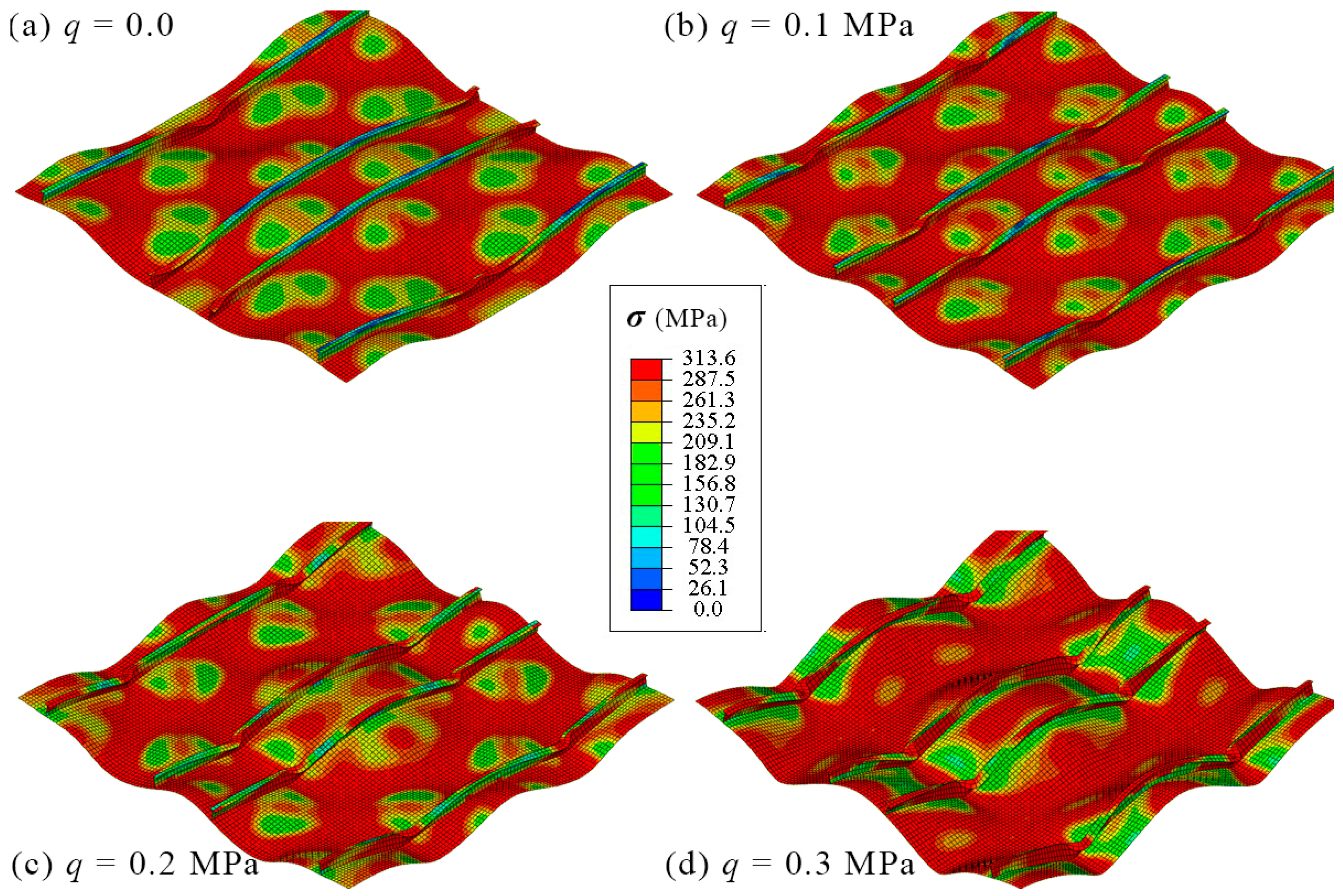
4.1. FE Model Validation

The validation case is based on an experimental study conducted by Estefen et al. [19]. In their research, the authors analyze a stiffened panel featuring seven identical longitudinal stiffeners, scaled at a ratio of 1:20, which resembles a typical panel found on a Suezmax tanker. The experimental specimen measures 200 mm in length, with its cross-section and thickness illustrated in Figure 4a. The material properties referenced from Ref. [19] consider σy = 381.4 MPa, E = 207.8 GPa, and ν = 0.3.
The original experimental study referenced in the study of [19] mapped the magnitudes and distributions of the initial geometric imperfections of the stiffened panels using portable measuring equipment. Additionally, the boundary conditions for the experimental case are represented in Figure 4b. For the FE validation, the initial deflections and their magnitudes take into account Equations (1)–(3), along with the considerations outlined in Section 2.2. Furthermore, the symmetry boundary conditions described in Figure 4c are also considered. A converged mesh with length l = 2 mm is adopted. The axial displacement and axial force distribution of the experimental, by Ref. [19], and numerical analysis conducted in this study are shown in Figure 5a. Finally, the final von Mises stress distribution of the post-collapsed stiffened panel is illustrated in Figure 5b.
The results presented in Figure 5a indicate that the stiffened panel from the experimental analysis demonstrates greater strength through deformation across a wider range compared to the numerical analysis in this study. Notably, the ultimate buckling load values are 143.77 kN for the experimental case and 135.22 kN for the numerical case, resulting in an MRE of 5.94%. These findings are consistent with the proposed objectives. Additionally, similarities in final deformation can be observed by comparing the experimental results in Ref. [19] with those shown in Figure 5b. Furthermore, Ref. [19] provides a numerical analysis that considers the mapping of initial imperfections, resulting in a ultimate buckling load of 136.08 kN, which shows an MRE of 0.63% when compared to the findings of the present study.

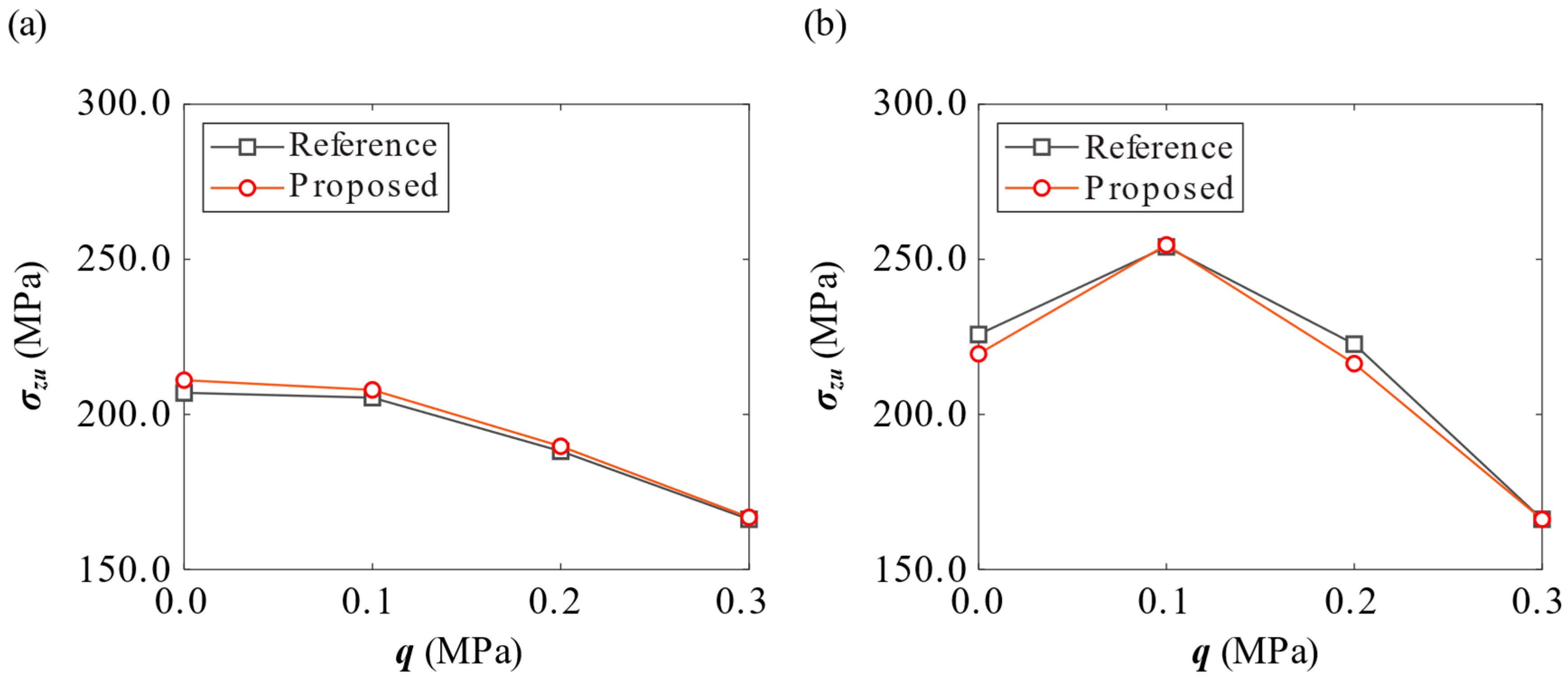
4.2. FE Model Verification

This paper aims to verify the application of the Finite Element Method (FEM) in real-world cases within the shipbuilding industry. Two stiffened panel cases, as presented by Xu et al. [10], are modeled for numerical analysis, incorporating periodic boundary conditions and mathematical initial deflections. The numerical results obtained are compared with the reference results.
The calculation specimens are denoted as P(tp)(dw × tw + bf × tf). The specimens P(9.5)(383 × 12 + 100 × 17) and P(22)(138 × 9 + 90 × 12) are adopted as a reference for FEM verification. Bulk carrier bottom-deck stiffened panels frequently experience a combination of in-plane compression and normal water pressure. To investigate the impact of lateral pressure on their strength capacity, four scenarios are analyzed. The first scenario served as a baseline with no lateral pressure (q = 0.0), while the remaining three scenarios incorporated lateral pressures of 0.1 MPa, 0.2 MPa, and 0.3 MPa.
Figure 6 compares the σzu to the q variation for the proposed verification cases. Table 2 presents the MRE obtained for each value of q. These results show similar values to those of the reference model.
Figure 7 illustrates the stress–strain curves of the stiffened panels subjected to combined loads at various water pressure levels. Figure 8 and Figure 9 depict the von Mises stress distributions as well as the deformed shapes of the two examples of stiffened panel specimens subjected to varying lateral load levels at ultimate strength.
As noted by Xu et al. [8] and Xu et al. [10], for the specimen depicted in Figure 4a, the σzu decreases as water pressure increases for the stiffened panels. However, in some cases, the σzu of the stiffened panels subjected to axial loads and q is more excellent than when pressure is not considered. In this context, Figure 8b illustrates a specimen where the σzu under pressure of q = 0.1 MPa exceeds the magnitude observed when q is not included.
The aptitude of lateral pressure to affect the σzu can vary based on several factors, including the applied load and the slenderness of the plate and the column. According to Xu et al. [10], normal pressure can have two opposing effects on the load-carrying capacity of stiffened panels subjected to combined loads. On one hand, they can increase collapse strength by enhancing buckling strength. On the other hand, they can also decrease collapse strength by diminishing yielding strength.

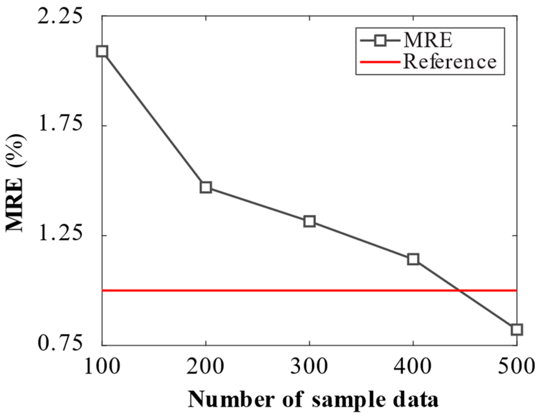
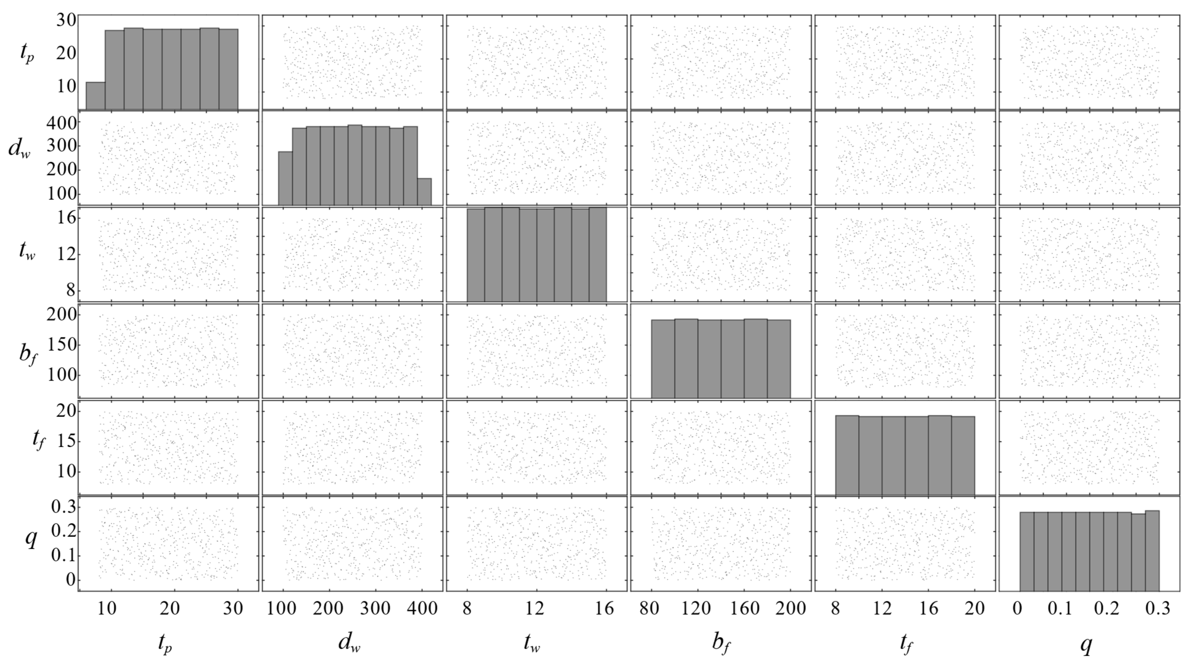
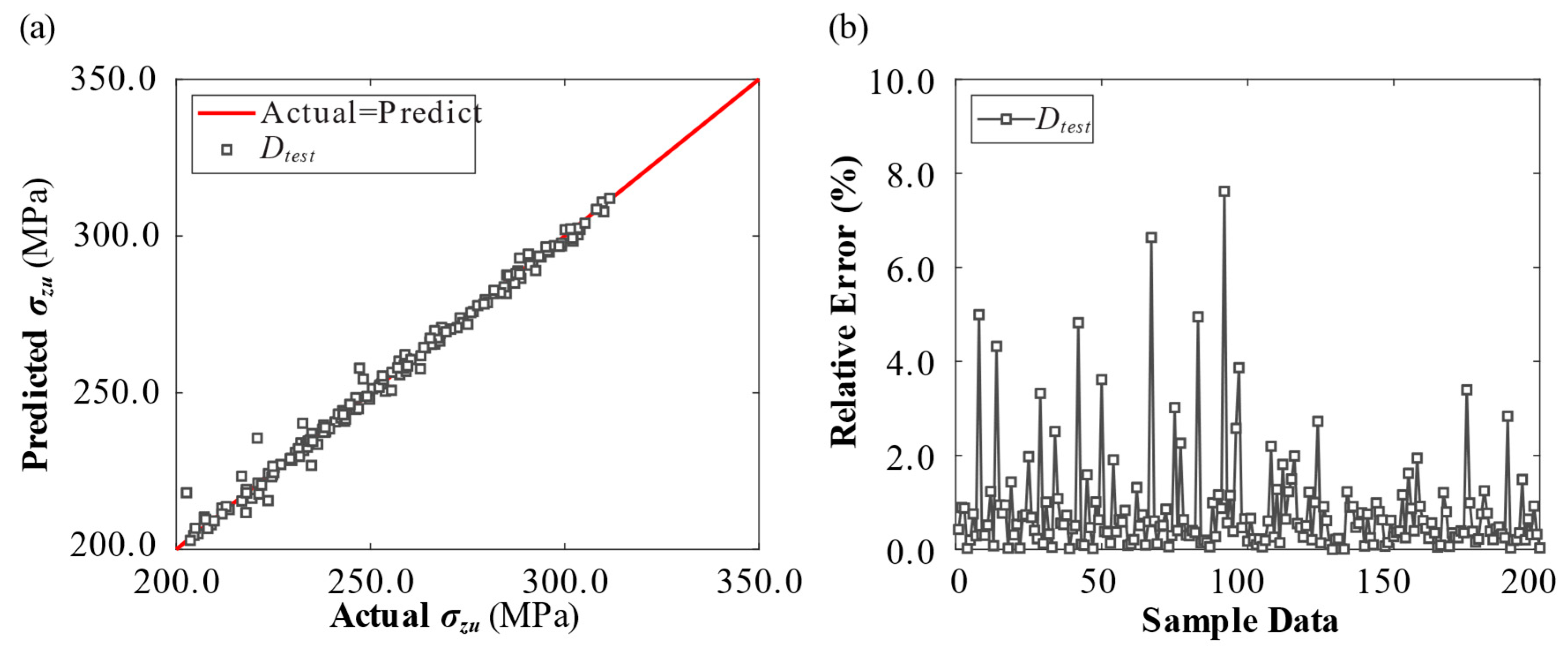
4.3. Kriging Surrogate Model for Collapse Assessment

This section examines the performance of the proposed Kriging surrogate model in predicting the σzu of stiffened panels subjected to combined loading based on finite element (FE) results. The accuracy of the σzu prediction is directly influenced by the number of support points ntrain associated with the optimized hyperparameters of the Kriging surrogate model.
Initially, the training points are set at ntrain = 100, and this value will be incrementally increased by 100 support points as needed until the stopping criterion of an MRE of 1% for the surrogate model is achieved. For each analysis, the best Kriging surrogate model is identified by applying GA to tune and optimize the hyperparameters using the training data. The lower and upper bounds for the surrogate hyperparameters, denoted as θ, are set in the interval [10−3, 103]. To evaluate the accuracy of the surrogate model, a total of test points is fixed at ntest = 200.
A sensitivity analysis is conducted to determine the GA parameters used to estimate the hyperparameters of each surrogate model. The initial population range of the stiffened panel geometry variables is defined within the lower and upper bounds outlined in Table 1. Additionally, the lateral pressure ranges from 0.0 to 0.3. The population sizes for the GA generations are evaluated at 25, 50, 100, and 200. The percentage of elite individuals who advance to the next generation is tested at 5%, 10%, 15%, and 20%. The crossover rate is set within a range of 0.5 and 1.0, varying in increments of 0.1.
The algorithm stops when any of these conditions are met: the maximum number of generations is set at 100 times the number of variables, culminating in a maximum of 600 generations, or the average relative change in the fitness function value over 30 generations falls below 1 × 10⁻⁶. Consequently, the sensitivity analysis for each Kriging surrogate model considers a total of 96 parameter combinations.
The criterion for selecting the best GA parameters is the total number of calls (Ncall) needed to meet the stopping criteria. Table 3 presents the results of the sensitivity analysis concerning the GA parameters for the different surrogate models.
The MRE and the accuracy considering Dtest on the Kriging surrogate model to predict σzu are depicted in Figure 10. The Kriging surrogate model initially did not achieve the desired precision with the specified number of support points ntrain = 100, resulting in an MRE of 2.1%. Additional support points are incrementally added to the training dataset until the model meets the stopping criterion of an MRE of 1%. It took four iterations to reach this goal, resulting in ntrain = 500 samples and an MRE of 0.82%. Figure 11 presents a scatter plot of 500 support points generated by the Latin Hypercube sampling method over the five iterations. The values of each variable appear to be uniformly distributed based on their probability distribution. Furthermore, the correlation distribution of variable values also shows a uniform pattern.
Figure 12a compares numerical σzu and σ*zu predictions made by Kriging using the Dtest dataset. The Dtest predictions align closely with the reference line, resulting in a high correlation coefficient of R2 = 0.9954. Figure 12b illustrates the relative error of σzu for each Dtest sample. As shown in Figure 12, the maximum and mean relative errors for all testing samples are 7.62% and 0.82%, respectively. Thus, the Kriging surrogate model demonstrates an adequate level of accuracy in predicting the σzu of the stiffened panels. Additionally, Figure 9b indicates that 91.5% of the Dtest samples have a relative error of less than 2%.

4.4. Kriging Hyperparameter Estimation

In the context of a high-dimensional nonlinear problem, visualizing the design landscape and understanding the effects of various variables can be quite challenging. The θ vector used in building the Kriging surrogate model does not fully capture the interactions between the variables. However, analyzing the components of θ makes it possible to identify the most significant variables and potentially eliminate less important ones from future optimization efforts. Figure 13 displays the hyperparameters θ obtained for the Kriging surrogate model.
This research investigates the sensitivity of stiffened panels by examining how variations in fundamental design parameters impact their behavior and collapse under combined loadings in various conditions. The stiffened panel model focuses explicitly on how uncertain factors—geometric irregularities and environmental loads—affect structural performance.
The variable ranking provided by the Kriging surrogate model (Figure 13) indicates that both geometric and environmental load variables significantly influence the σzu behavior of the stiffened panels. Among the factors considered, web height (dw) and plate thickness (tp) parameters (see Figure 1b) are the most critical for predicting σzu. Additionally, the lateral load (q) applied to the stiffened panel plays a substantial role in estimating σzu, particularly due to its relationship with the initial imperfections that affect the deformation of the panel’s shape. Other geometric variables, labeled bf, tw, and tf, rank lower in importance relative to the selected variables.

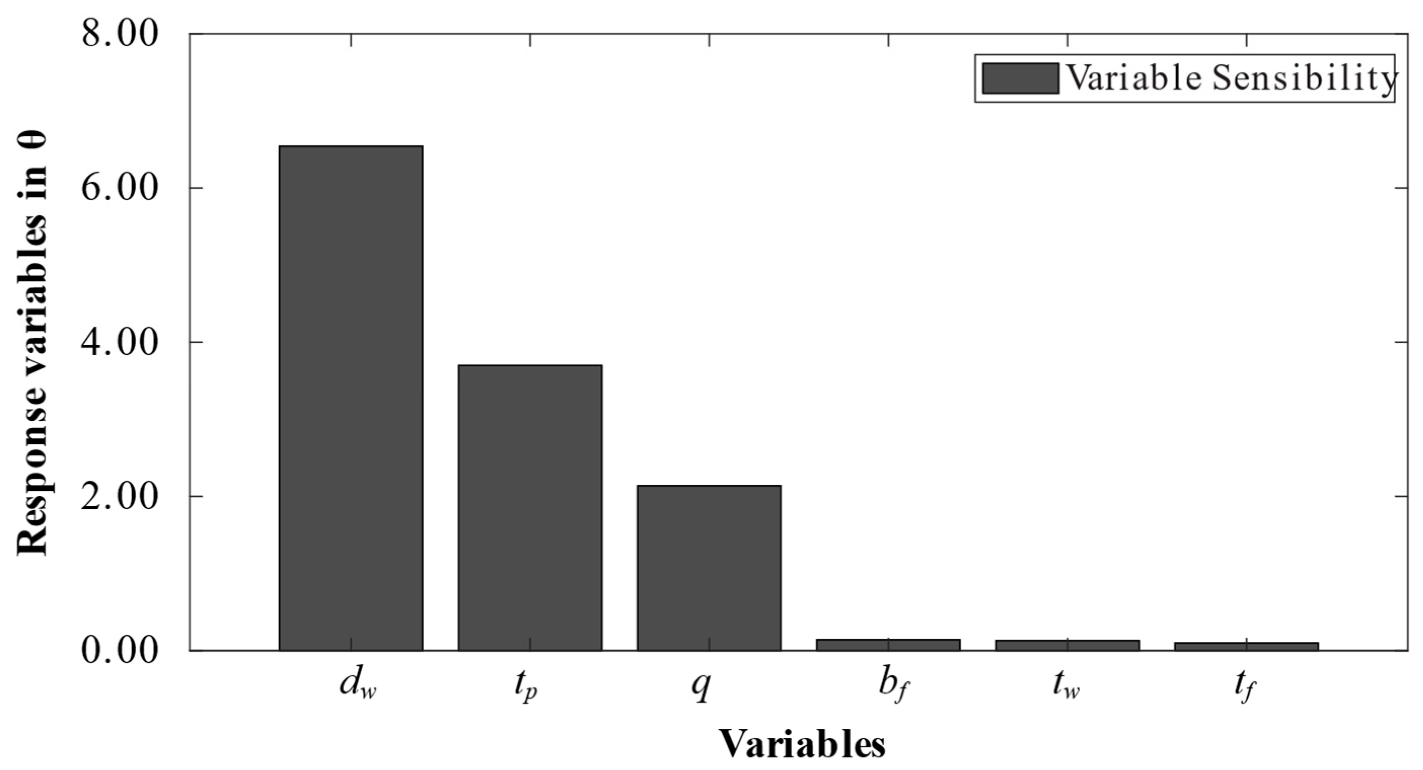
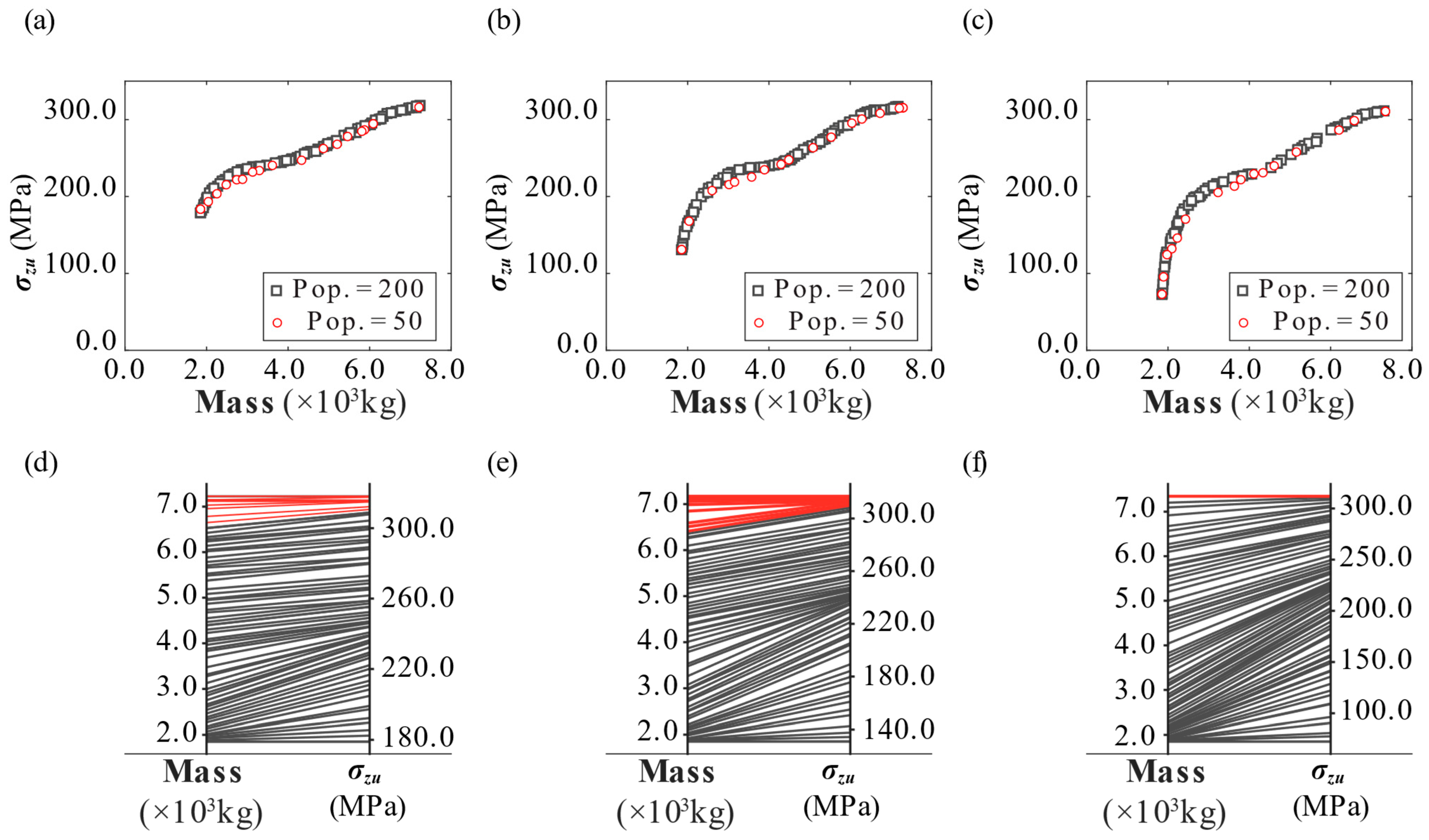
4.5. Multi-Objective Optimization in Ultimate Strength Behavior

This section illustrates the capability of the proposed Kriging surrogate model, which is based on the GA, to deliver optimized designs for σzu while considering the sensitivity of structural weight concerning mass (M). The value of M is obtained based on the volume of material used to construct the stiffened panel. Typically, a high sensitivity to design complexity will steer the optimization towards more straightforward layouts that are easier to construct. In a preliminary analysis, MOO is performed on three groups of stiffened panels, each with varying lateral pressure intervals: q ≤ 0.1 (Scenario 1); 0.1 < q ≤ 0.2 (Scenario 2), and 0.2 < q ≤ 0.3 (Scenario 3). The lateral pressure is considered a restriction of the MOO.
A sensitivity analysis is conducted to determine the NSGA-II parameters used to estimate the MOO of each lateral pressure scenario. The initial population range of the stiffened panel geometry variables is defined within the lower and upper bounds outlined in Table 1. Additionally, the lateral pressure ranges from 0.0 to 0.3. The population sizes for the NSGA generations are evaluated at 50, 100, and 200. The crossover probability is set within a range of 0.6 and 1.0, varying in increments of 0.1. The mutation probability is set within a range of 0.1 and 1.0, varying in increments of 0.1.
The algorithm stops when any of these conditions are met: the maximum number of generations is set at 100 times the number of variables, culminating in a maximum of 600 generations, or the final spread is less than the mean spread over the past 30 generations.
In all simulations of each scenario, the time required for the different parameter combinations is similar. Additionally, the Pareto curves are consistent across cases within the same scenario. Therefore, the criterion for selecting the best NSGA-II parameters is based on the total number of calls (Ncall) needed to satisfy the stopping criteria. Table 4 presents the sensitivity analysis results regarding the NSGA-II parameters for the various scenarios. A Pareto optimal solution is presented in Figure 14a–c for each scenario associated with a parallel plot in Figure 14d–f, which illustrates the trade-off between σzu and M.
Based on a sensitivity GA parameter analysis, a population of 50 individuals, associated with a Pareto fraction of 0.35, resulted in a Pareto front with individuals, making it difficult to establish the fundamental trade-off of the tension and mass relationship, in accord with Figure 14a–c. Therefore, when paired with the Pareto fraction, a population with 200 individuals is selected, as it provides better visualization of the Pareto front’s slopes without significantly increasing computation time.
The slope of the Pareto front for Scenario 1 (Figure 14a) progresses through four stages. In the first stage, σzu starts at approximately 180 MPa and increases rapidly until 225 MPa, while the structural mass begins at 1850 kg and increases at around 2500 kg. In the second stage, the slope increases gradually, reaching an M of 4300 kg when σzu is at 255 MPa. The third stage shows M values extending up to 6900 kg with σzu stabilizing around 310 MPa. Finally, in the last stage, the Pareto front stabilizes at σzu near 310 MPa, while the value of M increases to 7300 kg.
In Scenario 2 (Figure 14b) the σzu starts at approximately 130 MPa and increases rapidly to 210 MPa, while the structural mass begins at 1850 kg and increases at around 2600 kg. In the second stage, the slope increases gradually, reaching an M of 3900 kg when σzu is at 234 MPa. The third stage shows M values extending up to 6900 kg with σzu stabilizing around 310 MPa. Finally, in the last stage, the Pareto front stabilizes at σzu near 310 MPa, while the value of M increases to 7300 kg.
Scenario 3 (Figure 14c) is similar. Initially, the slope increases rapidly linearly, with the σzu ranging from 75 to 175 MPa, while M shows a modest increase, ranging from 1800 to 2100 kg. As the second slope develops, it gradually increases until M reaches 4600 kg at σzu = 250 MPa. In the subsequent stage, M values rise to a maximum of 6400 kg, with σzu remaining stable at around 310 MPa. In the final stage, the Pareto front stabilizes with σzu close to 310 MPa, but the mass parameter continues to increase, raising the value of M to 7300 kg.
Additionally, by examining the parallel graphs in Figure 14c–e, it is evident that Scenario 2 has stiffened panel geometric profiles, indicating higher load resistance capacities with strengths exceeding 310 MPa (red lines in the Figure 14d–f). This behavior is attributed to the fact that, during this stage, the lateral pressure benefits from the gain in resistance to axial compression. In contrast, Scenario 3 exhibits high lateral pressure values and has a relatively insignificant mass-resistance trade-off. Furthermore, the ultimate strength values are relatively low at less than 100 MPa during this stage.
According to the Pareto fronts depicted in Figure 14, all scenarios constrained by the q achieve high values of σzu, nearing σy = 313.6 MPa. The GA used to define the Pareto fronts in Figure 14 is also employed to select the geometry that ensures the minimum value of M while providing a maximum value of σzu ≥ 0.99σy, i.e., σzu ≥ 310 MPa.
This analysis evaluated how lateral pressure scenarios affect structural behavior while employing a GA optimization strategy. The MO problem is reformulated into a single-objective problem by incorporating the constraint that the maximum ultimate strength must be at least σzu ≥ 310 MPa.
The stiffened panel in a maximum σzu condition optimization starts with an initial population size of 1000. The selection process utilizes the roulette selection method, while the crossover operation employs a single-point crossover with a crossover probability of 0.8. To ensure the survival of high-performing individuals, the top 5% of the current population is preserved for the next generation. The algorithm stops when the weighted average change value of the fitness function falls below 1 × 10⁻⁶ or when the maximum number of generations, set at 150, is reached. Table 5 outlines the various scenarios of lateral pressure (q) along with their corresponding optimized points (x*) and the reduced mass (M) that yields the best structural performance in relation to σzu.
Table 5 demonstrates that the GA can determine the optimized value (x*) for each q scenario. In Scenario 1, the optimization process yields a stabilized estimated target σzu value obtained in the seventh GA evaluation, which results in a mass of M = 6480 kg. For Scenario 2, the sixth evaluation defines the optimization point with a mass of M = 6356 kg. For Scenario 3, the ninth evaluation establishes the optimization point with M = 6740 kg. In all three scenarios, the optimized geometry exhibits high values of tp, which is the main design variable influencing the determination of σzu. This pattern of optimized values is consistent with the results presented in Section 4.1, showing an initial gain in σzu at lower q values, followed by a decrease after a certain threshold for stiffened panels with a high value of the tp. Notably, Scenario 2 presents the highest σzu value at the lowest M value.

5. Conclusions

This study explored the potential of Kriging surrogate models for predicting the ultimate strength of stiffened panels subject to compressive uniaxial loads and lateral pressure, particularly in the context of highly nonlinear behavior. The results indicate that the Kriging surrogate framework applies to the collapse analysis of complex structures, providing an acceptable level of accuracy through optimizing hyperparameters via a GA. However, future works must realize comparative validation against alternative surrogate models to provide more substantial evidence for the model’s excellence.
The initial imperfections and geometry of the stiffened panels significantly influenced the ultimate strength of the specimens studied. Additionally, the panels exhibited varying collapse behaviors under the same geometric conditions when exposed to different external normal loads caused by water pressure. However, it is important to highlight that future efforts should focus on understanding how stiffened panels behave under biaxial loads and shear conditions, particularly regarding the predictability of the surrogate model. Additionally, research on material uncertainties should be linked to geometric variables to assess the surrogate model’s effectiveness. It is also crucial to assess the model’s universality by applying it to various types of vessels and new configurations of stiffened panels under different loading scenarios in future studies.
After the hyperparameters of the Kriging surrogate model were optimized, the model was trained on various combinations of training samples. Accuracy assessments were conducted to define the best sample configuration that yields a fitted model most representative of the collapse behavior. Furthermore, the ranking of design variables was established using the optimized Kriging surrogate model, which enabled an investigation into the significance of the selected variables in the surrogate response.
The analysis revealed that the Pareto front identified by the proposed methodology—combining the Kriging surrogate model with the NSGA-II algorithm—thoroughly examined the relationship between mass and ultimate strength. Additionally, the Genetic Algorithm optimization facilitated the formulation of a multi-objective problem that enabled the selection of an optimal geometric design to minimize the material mass while maximizing σzu, ultimately resulting in optimized mass across different lateral pressure scenarios.

Author Contributions

Conceptualization, J.P.S.L.; methodology, J.P.S.L.; software, J.P.S.L.; validation, J.P.S.L.; formal analysis, J.P.S.L.; investigation, J.P.S.L.; writing—original draft preparation, J.P.S.L.; writing—review and editing, J.P.S.L., R.L.V., E.D.d.S., L.A.O.R. and L.A.I.; visualization, J.P.S.L., R.L.V., E.D.d.S., L.A.O.R. and L.A.I.; supervision, E.D.d.S., L.A.O.R. and L.A.I. All authors have read and agreed to the published version of the manuscript.

Funding

This research was funded by the Brazilian Coordination for the Improvement of Higher Education Personnel—CAPES (finance code 001) and the Brazilian National Council for Scientific and Technological Development—CNPq (grant numbers: 308396/2021-9, 307791/2019-0, and 309648/2021-1).

Institutional Review Board Statement

Not applicable.

Informed Consent Statement

Not applicable.

Data Availability Statement

The original contributions presented in this study are included in the article. Further inquiries can be directed to the corresponding author.

Acknowledgments

The authors thank CAPES and CNPq for the financial support.

Conflicts of Interest

The authors declare no conflicts of interest.

Abbreviations

The following abbreviations are used in this manuscript:
aLength of local rectangular plates
A0Local plate initial deflection amplitude
bWidth of local rectangular plates
BWidth of the stiffened panels between girders
B0Column-type initial deflection amplitude
bfFlange breadth
C0Side-way initial deflection amplitude
CDCrowding-distance value
covCovariance
DtestObserved test dataset
DtrainObserved dataset
dwWeb height
EYoung’s modulus
f(x)Function
FEAFinite element analysis
G(x)Regression basis function
g(x)Multi-objective constraint
GAGenetic Algorithm
H’Strain hardening rate
mNumber of semi-waves in the plate
MMass
MLEMaximum Likelihood Estimation
MOEAMulti-objective Evolutionary Algorithm
MOPMulti-objective optimization problem
MREMean relative error
NSGANon-Sorting Genetic Algorithm
ntestObserved test dataset size
ntrainObserved dataset size
pKriging hyperparameter
PStiffened panel specimen
QLateral pressure
rx, ry, and rzRotational displacements around x, y, and z directions
tfFlange thickness
tpPlate thickness
twWeb thickness
ux, uy and uzTranslational displacements in x, y, and z directions
w0cColumn-type deflection of stiffeners
w0pInitial deflection of local plate panel
w0sSide-way deflection of stiffeners
X0Observed data
Y0Observed responses
Z(x)Regression Gaussian process error
βPlate slenderness
ηRegression coefficient
θKriging hyperparameter
μMean
σ2Variance
σYYield stress
σzuUltimate strength
υPoisson’s ratio
ψCorrelation
ΨCorrelation matrix

References

  1. Gaspar, B.; Naess, A.; Leira, B.J.; Soares, C.G. System Reliability Analysis of a Stiffened Panel under Combined Uniaxial Compression and Lateral Pressure Loads. Struct. Saf. 2012, 39, 30–43. [Google Scholar] [CrossRef]
  2. Song, Z.J.; Liu, Q.C.; Xu, R.J.; Yang, X.; Yue, J.X. Ultimate Strength Attenuation Behaviours of Stiffened Panels under Cyclic Extreme Loads Based on Test and Numerical Simulations. Ocean Eng. 2025, 321, 120447. [Google Scholar] [CrossRef]
  3. Wang, X.; Moan, T. Ultimate Strength Analysis of Stiffened Panels in Ships Subjected to Biaxial and Lateral Loading. Int. J. Offshore Polar Eng. 1996, 7, 22–29. [Google Scholar]
  4. Soares, C.G.; Gordo, J.M. Compressive Strength of Rectangular Plates under Biaxial Load and Lateral Pressure. Thin-Walled Struct. 1996, 24, 231–259. [Google Scholar] [CrossRef]
  5. Fujikubo, M.; Harada, M.; Yao, T.; Reza Khedmati, M.; Yanagihara, D. Estimation of Ultimate Strength of Continuous Stiffened Panel under Combined Transverse Thrust and Lateral Pressure Part 2: Continuous Stiffened Panel. Mar. Struct. 2005, 18, 411–427. [Google Scholar] [CrossRef]
  6. Benson, S.; Downes, J.; Dow, R.S. Overall Buckling of Lightweight Stiffened Panels Using an Adapted Orthotropic Plate Method. Eng. Struct. 2015, 85, 107–117. [Google Scholar] [CrossRef]
  7. Li, S.; Hu, Z.; Benson, S. An Analytical Method to Predict the Buckling and Collapse Behaviour of Plates and Stiffened Panels under Cyclic Loading. Eng. Struct. 2019, 199, 109627. [Google Scholar] [CrossRef]
  8. Xu, M.C.; Yanagihara, D.; Fujikubo, M.; Soares, C.G. Influence of Boundary Conditions on the Collapse Behaviour of Stiffened Panels under Combined Loads. Mar. Struct. 2013, 34, 205–225. [Google Scholar] [CrossRef]
  9. Tanaka, S.; Yanagihara, D.; Yasuoka, A.; Harada, M.; Okazawa, S.; Fujikubo, M.; Yao, T. Evaluation of Ultimate Strength of Stiffened Panels under Longitudinal Thrust. Mar. Struct. 2014, 36, 21–50. [Google Scholar] [CrossRef]
  10. Xu, M.C.; Song, Z.J.; Pan, J.; Soares, C.G. Ultimate Strength Assessment of Continuous Stiffened Panels under Combined Longitudinal Compressive Load and Lateral Pressure. Ocean Eng. 2017, 139, 39–53. [Google Scholar] [CrossRef]
  11. Han, P.; Ri, K.; Yun, C.; Pak, C.; Paek, S. A Study on the Residual Ultimate Strength of Continuous Stiffened Panels with a Crack under the Combined Lateral Pressure and in-Panel Compression. Ocean Eng. 2021, 234, 109265. [Google Scholar] [CrossRef]
  12. Barsotti, B.; Battini, C.; Gaiotti, M.; Rizzo, C.M.; Vergassola, G. Experimental and Numerical Assessment of Ultimate Strength of a Transversally Loaded Thin-Walled Deck Structure. Mar. Struct. 2025, 103, 103793. [Google Scholar] [CrossRef]
  13. Ringsberg, J.W.; Darie, I.; Nahshon, K.; Shilling, G.; Vaz, M.A.; Benson, S.; Brubak, L.; Feng, G.; Fujikubo, M.; Gaiotti, M.; et al. The ISSC 2022 Committee Iii.1-Ultimate Strength Benchmark Study on the Ultimate Limit State Analysis of a Stiffened Plate Structure Subjected to Uniaxial Compressive Loads. Mar. Struct. 2021, 79, 103026. [Google Scholar] [CrossRef]
  14. Kim, D.K.; Lim, H.L.; Kim, M.S.; Hwang, O.J.; Park, K.S. An Empirical Formulation for Predicting the Ultimate Strength of Stiffened Panels Subjected to Longitudinal Compression. Ocean Eng. 2017, 140, 270–280. [Google Scholar] [CrossRef]
  15. Benson, S.; Downes, J.; Dow, R.S. Ultimate Strength Characteristics of Aluminium Plates for High-Speed Vessels. Ships Offshore Struct. 2011, 6, 67–80. [Google Scholar] [CrossRef]
  16. Paik, J.K.; Kim, B.J.; Seo, J.K. Methods for Ultimate Limit State Assessment of Ships and Ship-Shaped Offshore Structures: Part Ii Stiffened Panels. Ocean Eng. 2008, 35, 271–280. [Google Scholar] [CrossRef]
  17. Khedmati, M.R.; Pedram, M.; Rigo, P. The Effects of Geometrical Imperfections on the Ultimate Strength of Aluminium Stiffened Plates Subject to Combined Uniaxial Compression and Lateral Pressure. Ships Offshore Struct. 2014, 9, 88–109. [Google Scholar] [CrossRef]
  18. Li, S.; Georgiadis, D.G.; Kim, D.K.; Samuelides, M.S. A Comparison of Geometric Imperfection Models for Collapse Analysis of Ship-Type Stiffened Plated Grillages. Eng. Struct. 2022, 250, 113480. [Google Scholar] [CrossRef]
  19. Estefen, S.F.; Chujutalli, J.H.; Soares, C.G. Influence of Geometric Imperfections on the Ultimate Strength of the Double Bottom of a Suezmax Tanker. Eng. Struct. 2016, 127, 287–303. [Google Scholar] [CrossRef]
  20. Doan, V.T.; Liu, B.; Garbatov, Y.; Wu, W.; Soares, C.G. Strength Assessment of Aluminium and Steel Stiffened Panels with Openings on Longitudinal Girders. Ocean Eng. 2020, 200, 107047. [Google Scholar] [CrossRef]
  21. Saad-Eldeen, S.; Garbatov, Y.; Soares, C.G. Experimental Failure Assessment of High Tensile Stiffened Plates with Openings. Eng. Struct. 2020, 206, 110121. [Google Scholar] [CrossRef]
  22. Kim, D.K.; Kim, S.J.; Kim, H.B.; Zhang, X.M.; Li, C.G.; Paik, J.K. Ultimate Strength Performance of Bulk Carriers with Various Corrosion Additions. Ship Offshore Struct. 2015, 10, 59–78. [Google Scholar] [CrossRef]
  23. Cui, J.; Wang, D.; Ma, N. Case Studies on the Probabilistic Characteristics of Ultimate Strength of Stiffened Panels with Uniform and Non-Uniform Localized Corrosion Subjected to Uniaxial and Biaxial Thrust. Int. J. Nav. Archit. Ocean Eng. 2019, 11, 97–118. [Google Scholar] [CrossRef]
  24. Feng, L.; Hu, L.; Chen, X.; Shi, H. A Parametric Study on Effects of Pitting Corrosion on Stiffened Panels’ Ultimate Strength. Int. J. Nav. Archit. Ocean Eng. 2020, 12, 699–710. [Google Scholar] [CrossRef]
  25. Feng, G.Q.; Garbatov, Y.; Soares, C.G. Probabilistic Model of the Growth of Correlated Cracks in a Stiffened Panel. Eng. Fract. Mech. 2012, 84, 83–95. [Google Scholar] [CrossRef]
  26. Xu, M.C.; Garbatov, Y.; Soares, C.G. Residual Ultimate Strength Assessment of Stiffened Panels with Locked Cracks. Thin-Walled Struct. 2014, 85, 398–410. [Google Scholar] [CrossRef]
  27. Bucher, C.G.; Bourgund, U. A Fast and Efficient Response Surface Approach for Structural Reliability Problems. Struct. Saf. 1990, 7, 57–66. [Google Scholar] [CrossRef]
  28. Rajashekhar, M.R.; Ellingwood, B.R. A New Look at the Response Surface Approach for Reliability Analysis. Struct. Saf. 1993, 12, 205–220. [Google Scholar] [CrossRef]
  29. Bypour, M.; Kioumarsi, M.; Yekrangnia, M. Shear Capacity Prediction of Stiffened Steel Plate Shear Walls (Sspsw) with Openings Using Response Surface Method. Eng. Struct. 2021, 226, 111340. [Google Scholar] [CrossRef]
  30. Gaspar, B.; Bucher, C.; Soares, C.G. Reliability Analysis of Plate Elements under Uniaxial Compression Using an Adaptive Response Surface Approach. Ships Offshore Struct. 2014, 10, 145–161. [Google Scholar] [CrossRef]
  31. Firtikiadis, L.; Tzotzis, A.; Kyratsis, P.; Efkolidis, N. Response Surface Methodology (Rsm)-Based Evaluation of the 3d-Printed Recycled-Petg Tensile Strength. Appl. Mech. 2024, 5, 924–937. [Google Scholar] [CrossRef]
  32. Khatibinia, M.; Jalaipour, M.; Gharehbaghi, S. Shape Optimization of U-Shaped Steel Dampers Subjected to Cyclic Loading Using an Efficient Hybrid Approach. Eng. Struct. 2019, 197, 108874. [Google Scholar] [CrossRef]
  33. Jiang, W.; Xie, Y.; Li, W.; Wu, J.; Long, G. Prediction of the Splitting Tensile Strength of the Bonding Interface by Combining the Support Vector Machine with the Particle Swarm Optimization Algorithm. Eng. Struct. 2021, 230, 111696. [Google Scholar] [CrossRef]
  34. Lim, H.; Manuel, L.; Low, Y.M.; Srinil, N. A Surrogate Model for Estimating Uncertainty in Marine Riser Fatigue Damage Resulting from Vortex-Induced Vibration. Eng. Struct. 2022, 254, 113796. [Google Scholar] [CrossRef]
  35. Hariri-Ardebili, M.A.; Sudret, B. Polynomial Chaos Expansion for Uncertainty Quantification of Dam Engineering Problems. Eng. Struct. 2020, 203, 109631. [Google Scholar] [CrossRef]
  36. Prem, M.S.; Klanner, M.; Ellermann, K. Identification of Fractional Damping Parameters in Structural Dynamics Using Polynomial Chaos Expansion. Appl. Mech. 2021, 2, 956–975. [Google Scholar] [CrossRef]
  37. Wan, H.-P.; Mao, Z.; Todd, M.D.; Ren, W.-X. Analytical Uncertainty Quantification for Modal Frequencies with Structural Parameter Uncertainty Using a Gaussian Process Metamodel. Eng. Struct. 2014, 75, 577–589. [Google Scholar] [CrossRef]
  38. Heng, J.; Zhou, Z.; Zou, Y.; Kaewunruen, S. Gpr-Assisted Evaluation of Probabilistic Fatigue Crack Growth in Rib-to-Deck Joints in Orthotropic Steel Decks Considering Mixed Failure Models. Eng. Struct. 2022, 252, 113688. [Google Scholar] [CrossRef]
  39. Yetilmezsoy, K.; Sihag, P.; Kıyan, E.; Doran, B. A Benchmark Comparison and Optimization of Gaussian Process Regression, Support Vector Machines, and M5p Tree Model in Approximation of the Lateral Confinement Coefficient for Cfrp-Wrapped Rectangular/Square Rc Columns. Eng. Struct. 2021, 246, 113106. [Google Scholar] [CrossRef]
  40. Chojaczyk, A.A.; Teixeira, A.P.; Neves, L.C.; Cardoso, J.B.; Soares, C.G. Review and Application of Artificial Neural Networks Models in Reliability Analysis of Steel Structures. Struct. Saf. 2015, 52, 78–89. [Google Scholar] [CrossRef]
  41. Lima, J.P.S.; Evangelista, F.; Soares, C.G. Hyperparameter-Optimized Multi-Fidelity Deep Neural Network Model Associated with Subset Simulation for Structural Reliability Analysis. Reliab. Eng. Syst. Saf. 2023, 239, 109492. [Google Scholar] [CrossRef]
  42. Tahir, Z.U.R.; Mandal, P.; Adil, M.T.; Naz, F. pplication of Artificial Neural Network to Predict Buckling Load of Thin Cylindrical Shells under Axial Compression. Eng. Struct. 2021, 248, 113221. [Google Scholar] [CrossRef]
  43. Yoo, K.; Bacarreza, O.; Aliabadi, M.H.F. A Novel Multi-Fidelity Modelling-Based Framework for Reliability-Based Design Optimisation of Composite Structures. Eng. Comput. 2020, 38, 595–608. [Google Scholar] [CrossRef]
  44. Gaspar, B.; Teixeira, A.P.; Soares, C.G. Assessment of the Efficiency of Kriging Surrogate Models for Structural Reliability Analysis. Probabilistic Eng. Mech. 2014, 37, 24–34. [Google Scholar] [CrossRef]
  45. Das, S.; Tesfamariam, S. Optimization of Sma Based Damped Outrigger Structure under Uncertainty. Eng. Struct. 2020, 222, 111074. [Google Scholar] [CrossRef]
  46. Lu, P.; Xu, Z.; Chen, Y.; Zhou, Y. Prediction Method of Bridge Static Load Test Results Based on Kriging Model. Eng. Struct. 2020, 214, 110641. [Google Scholar] [CrossRef]
  47. Qiu, Y.; Yu, R.; San, B.; Li, J. Aerodynamic Shape Optimization of Large-Span Coal Sheds for Wind-Induced Effect Mitigation Using Surrogate Models. Eng. Struct. 2022, 253, 113818. [Google Scholar] [CrossRef]
  48. Maitra, V.; Shi, J. Kriging Metamodel-Based Multi-Objective Optimization for Laser-Powder Bed Fusion of Ti-6al-4v Alloy. J. Manuf. Process. 2025, 137, 45–67. [Google Scholar] [CrossRef]
  49. Li, Y.; Wang, S.; Wu, Y.; Zhang, Z.; Shen, J. A Global Optimization Method Based on Fuzzy Clustering Kriging for Aerobic Wastewater Treatment. J. Environ. Manag. 2025, 380, 125163. [Google Scholar] [CrossRef]
  50. Xiao, X.; Li, Q.; Zhang, H. Efficient Kriging-Based Wall Deflection Prediction in Braced Excavation Considering Model and Measurement Errors. Eng. Appl. Artif. Intell. 2025, 149, 110506. [Google Scholar] [CrossRef]
  51. Liu, P.; Shang, D.; Liu, Q.; Yi, Z.; Wei, K. Kriging Model for Reliability Analysis of the Offshore Steel Trestle Subjected to Wave and Current Loads. J. Mar. Sci. Eng. 2022, 10, 25. [Google Scholar] [CrossRef]
  52. Ye, X.; Zheng, P.; Qiao, D.; Zhao, X.; Zhou, Y.; Wang, L. Multi-Objective Optimization Design of a Mooring System Based on the Surrogate Model. J. Mar. Sci. Eng. 2024, 12, 1853. [Google Scholar] [CrossRef]
  53. Shi, X.; Teixeira, Â.P.; Zhang, J.; Soares, C.G. Kriging Response Surface Reliability Analysis of a Ship-Stiffened Plate with Initial Imperfections. Struct. Infrastruct. Eng. 2014, 11, 1450–1465. [Google Scholar] [CrossRef]
  54. Lima, J.P.S.; Evangelista, F.; Soares, C.G. Bi-Fidelity Kriging Model for Reliability Analysis of the Ultimate Strength of Stiffened Panels. Mar. Struct. 2023, 91, 103464. [Google Scholar] [CrossRef]
  55. Wu, Q.; Hu, S.; Tang, X.; Liu, X.; Chen, Z.; Xiong, J. Compressive Buckling and Post-Buckling Behaviors of J-Type Composite Stiffened Panel before and after Impact Load. Compos. Struct. 2023, 304, 116339. [Google Scholar] [CrossRef]
  56. Lian, C.; Wang, P.; Zhang, K.; Yuan, K.; Zheng, J.; Yue, Z. Experimental and Numerical Research on the Calculation Methods for Buckling and Post-Buckling of Aircraft Tail Inclined Stiffened Panel under Compression Load. Aerosp. Sci. Technol. 2024, 146, 108930. [Google Scholar] [CrossRef]
  57. Aguiari, M.; Gaiotti, M.; Rizzo, C.M. A Design Approach to Reduce Hull Weight of Naval Ships. Ship Technol. Res. 2022, 69, 89–104. [Google Scholar] [CrossRef]
  58. ISSC. Report of Specialist Committee III.1 Ultimate Strength. In Proceedings of the 18th International Ship and Offshore Structures Congress, Rostock, Germany, 9–13 September 2012. [Google Scholar]
  59. Ueda, Y.; Yao, T. The Influence of Complex Initial Deflection Modes on the Behaviour and Ultimate Strength of Rectangular Plates in Compression. J. Constr. Steel Res. 1985, 5, 265–302. [Google Scholar] [CrossRef]
  60. Soares, C.G. Design Equation for the Compressive Strength of Unstiffened Plate Elements with Initial Imperfections. J. Constr. Steel Res. 1988, 9, 287–310. [Google Scholar] [CrossRef]
  61. Kmiecik, M.; Jastrzebski, T.; Kuzniar, J. Statistics of Ship Plating Distortions. Mar. Struct. 1995, 8, 119–132. [Google Scholar] [CrossRef]
  62. Yuan, T.; Yang, Y.; Kong, X.; Wu, W. Similarity Criteria for the Buckling Process of Stiffened Plates Subjected to Compressive Load. Thin-Walled Struct. 2021, 158, 107183. [Google Scholar] [CrossRef]
  63. Garud, S.S.; Karimi, I.A.; Kraft, M. Design of Computer Experiments: A Review. Comput. Chem. Eng. 2017, 106, 71–95. [Google Scholar] [CrossRef]
  64. Krige, D.G. A Statistical Approaches to Some Basic Mine Valuation Problems on the Witwatersrand. J. Chem. Metall. Min. Soc. S. Afr. 1951, 52, 119–139. [Google Scholar]
  65. Forrester, A.I.; Sóbester, A.; Keane, A.J. Multi-Fidelity Optimization Via Surrogate Modelling. Proc. R. Soc. Lond. A Math. Phys. Eng. Sci. 2007, 463, 3251–3269. [Google Scholar] [CrossRef]
  66. Goldberg, D.E. Genetic Algorithms in Search, Optimization & Machine Learning; Addison-Wesley: Boston, MA, USA, 1989. [Google Scholar]
  67. Eiben, A.E.; Smith, J.E. Introduction to Evolutionary Computing, 2nd ed.; Springer: Berlin/Heidelberg, Germany, 2015. [Google Scholar]
  68. Deb, K.; Agrawal, S.; Pratap, A.; Meyarivan, T. A Fast Elitist Non-dominated Sorting Genetic Algorithm for Multi-objective Optimization: Nsga-Ii. In Parallel Problem Solving from Nature PPSN VI; Springer: Berlin/Heidelberg, Germany, 2000. [Google Scholar]
  69. Deb, K. Multi-Objective Optimization Using Evolutionary Algorithms; Wiley: Chichester, UK, 2001; p. 536. [Google Scholar]
  70. Kumar, H.; Yadav, S.P. Hybrid Nsga-Ii Based Decision-Making in Fuzzy Multi-Objective Reliability Optimization Problem. SN Appl. Sci. 2019, 1, 1496. [Google Scholar] [CrossRef]
  71. Guo, Y.; Wang, Y.; Cao, Y.; Long, Z. A New Optimization Design Method of Multi-Objective Indoor Air Supply Using the Kriging Model and NSGA-II. Appl. Sci. 2023, 13, 10465. [Google Scholar] [CrossRef]
  72. Duran-Castillo, A.; Jauregui-Correa, J.C.; Benítez-Rangel, J.P.; Dominguez-Gonzalez, A.; De Santiago, O.C. Multi-Objective Optimization Design of Porous Gas Journal Bearing Considering the Fluid–Structure Interaction Effect. Appl. Mech. 2024, 5, 600–618. [Google Scholar] [CrossRef]
Figure 1. Stiffened panels: (a) Schematic view of a stiffened panel. (b) Stiffener section view. (c) Typical stiffened panel in ship structure and its modeling extent.
Applmech 06 00034 g001
Figure 2. Initial deflection shapes of (a) local plate panel imperfection; (b) column-type imperfection; (c) side-way stiffener imperfection; and (d) association of the initial deflection shapes with mean amplitude scale factor 50×.
Applmech 06 00034 g002
Figure 3. Overall GA-MOEA optimization using Kriging surrogate methodology flowchart.
Applmech 06 00034 g003
Figure 4. Experimental stiffened panel specimen: (a) Cross-section and dimensions in mm. (b) Boundary conditions. (c) Numerical boundary conditions.
Applmech 06 00034 g004
Figure 5. Buckling behavior: (a) Buckling force versus axial displacement curves and (b) post-collapse mode for numerical model.
Applmech 06 00034 g005
Figure 6. The ultimate strength of the reference stiffened panels with different lateral load scenarios: (a) P(9.5)(383 × 12 + 100 × 17) and (b) P(22)(138 × 9 + 90 × 12).
Applmech 06 00034 g006
Figure 7. Stress–strain curves of the stiffened panels with different water pressure levels: (a) P(9.5)(383 × 12 + 100 × 17) and (b) P(22)(138 × 9 + 90 × 12).
Applmech 06 00034 g007
Figure 8. Deformed shapes of stiffened panel P(9.5)(383 × 12 + 100 × 17) (scale factor ×20) with (a) no lateral pressure (q = 0.0); (b) q = 0.1 MPa; (c) q = 0.2 MPa; and (d) q = 0.3 MPa.
Applmech 06 00034 g008
Figure 9. Deformed shapes of stiffened panel P(22)(138 × 9 + 90 × 12) (scale factor ×20) with (a) no lateral pressure (q = 0.0); (b) q = 0.1 MPa; (c) q = 0.2 MPa; and (d) q = 0.3 MPa.
Applmech 06 00034 g009
Figure 10. The tendency of the global of the Kriging surrogate model MRE.
Applmech 06 00034 g010
Figure 11. Scatter matrix plot of the variables’ spatial distribution.
Applmech 06 00034 g011
Figure 12. Approximation of the σzu: (a) Using Kriging surrogate model. (b) Relative error in the σzu.
Applmech 06 00034 g012
Figure 13. Ranking of variable importance generated by Kriging hyperparameter optimization.
Applmech 06 00034 g013
Figure 14. Pareto front solution for the σzu vs. mass correlation in (a) Scenario 1; (b) Scenario 2; and (c) Scenario 3. Parallel coordinate plot of the approximate Pareto front on the (d) Scenario 1; (e) Scenario 2; and (f) Scenario 3 case. The red lines indicate higher load resistance capacities cases with strengths exceeding 310 MPa and the black lines indicate the other cases.
Applmech 06 00034 g014
Table 1. Description of the geometrical stiffened panel basic variables.
VariableUnitsDescriptionLower BoundUpper Bound
tpmmPlate thickness8.030.0
dwmmWeb height100.0400.0
tfmmFlange thickness8.020.0
bfmmFlange breadth80.0200.0
twmmWeb thickness8.016.0
Table 2. Relative error of each verification model specimen.
Specimenq (MPa)
0.00.10.20.3
MRE (%)
P(9.5)(383 × 12 + 100 × 17)1.961.220.830.37
P(22)(138 × 9 + 90 × 12)2.770.242.810.01
Table 3. Selected GA parameters for the different surrogate models.
ntrainPopulation SizeElite Fraction (%)Crossover FractionObjective Function (MLE)Computational Time (seg)GenerationsNcall
10010050.7282.447868275
20010050.6583.3162827895
30010050.7894.0514979320
40020050.8129569818115,600
50020050.81561.111,2719418,070
Table 4. Specifications of the NSGA-II-parameters.
ScenarioPopulation SizeCrossover FractionMutation RateGenerationsNcallTime
1200 (50)0.7 (0.8)0.3 (0.3)102 (112)20,400 (5600)30.55 (9.33)
2200 (50)0.7 (0.9)0.3 (0.4)102 (106)20,400 (5300)30.85 (9.84)
3200 (50)0.9 (0.8)0.4 (0.2)102 (102)20,400 (5100)30.65 (8.55)
Table 5. Optimized point in each lateral pressure range.
Scenario (MPa)x*
tp (mm)dw (mm)tf (mm)bf (mm)tw (mm)q (MPa)M (kg)
0.0 ≤ q1 ≤ 0.128.83222.4812.74138.838.000.096480.0
0.1 < q2 ≤ 0.228.68183.4613.24117.848.000.136356.0
0.2 < q3 ≤ 0.330.00184.0013.38144.4011.410.206740.0
Disclaimer/Publisher’s Note: The statements, opinions and data contained in all publications are solely those of the individual author(s) and contributor(s) and not of MDPI and/or the editor(s). MDPI and/or the editor(s) disclaim responsibility for any injury to people or property resulting from any ideas, methods, instructions or products referred to in the content.

