An Analytical Solution for Natural Frequencies of Elastically Supported Stepped Beams with Rigid Segments

Abstract
1. Introduction
2. Materials and Methods
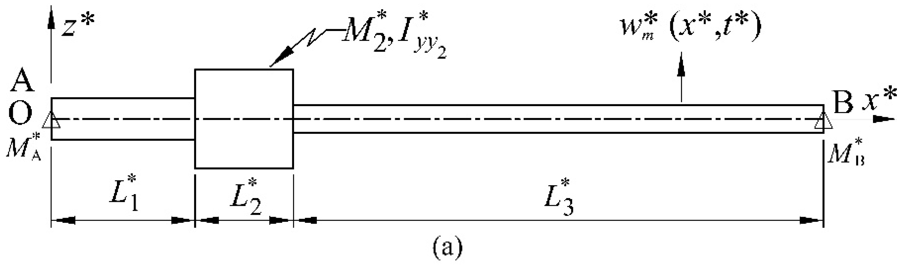
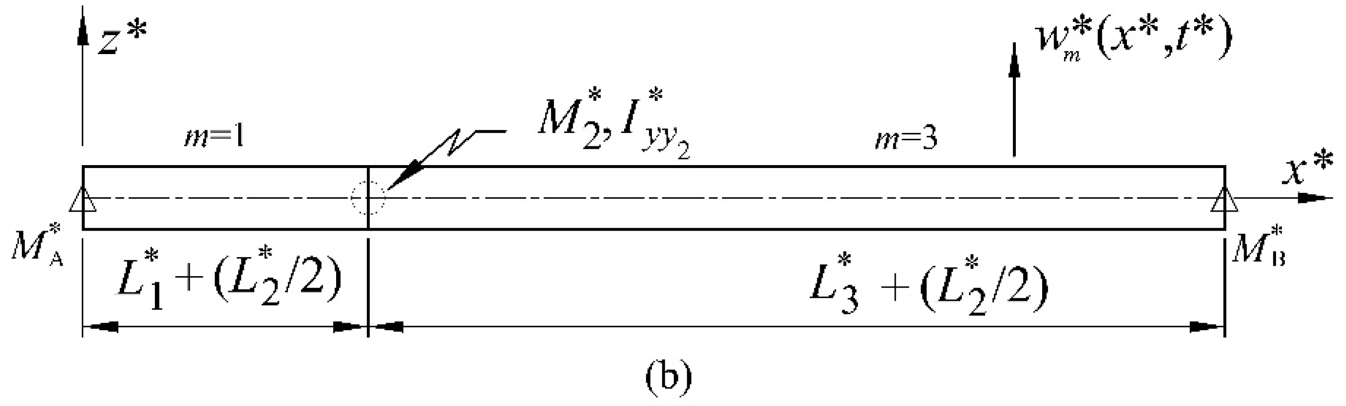
2.1. Formulation of the Problem
2.1.1. Dimensionless Equations of Motion
2.1.2. Separation of Variables and Resulting Equations
2.2. Solution Method for Eigenvalues
2.3. Verifications
2.3.1. Verification 1
2.3.2. Verification 2
2.3.3. Verification 3
3. Results
3.1. Numerical Applications
3.1.1. Case 1
3.1.2. Case 2
3.1.3. Case 3
3.2. Graphical Presentations and Discussions
3.2.1. Presentation 1
3.2.2. Presentation 2
3.2.3. Presentation 3
3.2.4. Presentation 4
3.2.5. Presentation 5
3.2.6. Presentation 6
4. Discussion
Funding
Institutional Review Board Statement
Informed Consent Statement
Data Availability Statement
Acknowledgments
Conflicts of Interest
Appendix A
References
- Kopmaz, O.; Telli, S. On the Eigenfrequencies of a Two-Part Beam–Mass System. J. Sound Vib. 2002, 252, 370–384. [Google Scholar] [CrossRef]
- Taleb, N.J.; Suppiger, E.W. Vibration of Stepped Beams. J. Aerosp. Eng. 1961, 28, 295–298. [Google Scholar] [CrossRef]
- Balasubramanian, T.S.; Subramanian, G. On the performance of a four-degree-of-freedom per node element for stepped beam analysis and higher frequency estimation. J. Sound Vib. 1985, 99, 563–567. [Google Scholar] [CrossRef]
- Subramanian, G.; Balasubramanian, T.S. Beneficial effects of steps on the free vibration characteristics of beams. J. Sound Vib. 1987, 118, 555–560. [Google Scholar] [CrossRef]
- Sarıgül, A.S.; Aksu, G. A finite difference method for the free vibration analysis of stepped Timoshenko beams and shafts. Mech. Mach. Theory 1986, 21, 1–12. [Google Scholar] [CrossRef]
- Jang, S.K.; Bert, C.W. Free Vibration of Stepped Beams: Exact and Numerical Solutions. J. Sound Vib. 1989, 130, 342–346. [Google Scholar] [CrossRef]
- Özkaya, E.; Pakdemirli, M.; Öz, H.R. Non-Liner Vibrations of a Beam–Mass System Under Different Boundary Conditions. J. Sound Vib. 1997, 199, 679–696. [Google Scholar] [CrossRef]
- Magrab, E.B. Vibrations of Elastic Systems with Applications to MEMS and NEMS; Springer: Dordrecht/Heidelberg, Germany, 2012. [Google Scholar]
- Kopmaz, O.; Telli, S. Authors’ reply. J. Sound Vib. 2003, 265, 911–916. [Google Scholar] [CrossRef]
- Naguleswaran, S. Vibration of an Euler–Bernoulli stepped beam carrying a non-symmetrical rigid body at the step. J. Sound Vib. 2004, 271, 1121–1132. [Google Scholar] [CrossRef]
- Ilanko, S. Transcendental Dynamic Stability Functions for Beams Carrying Rigid Bodies. J. Sound Vib. 2005, 279, 1195–1202. [Google Scholar] [CrossRef]
- Lin, H.-Y.; Wang, C.-Y. Free Vibration Analysis of a Hybrid Beam Composed of Multiple Elastic Beam Segments and Elastic-Supported Rigid Bodies. J. Mar. Sci. Technol. 2012, 20, 525–533. [Google Scholar] [CrossRef]
- Obradovic, A.; Salinic, S.; Trifkovic, D.R.; Zoric, N.; Stokic, Z. Free vibration of structures composed of rigid bodies and elastic beam segments. J. Sound Vib. 2015, 347, 126–138. [Google Scholar] [CrossRef]
- Farghaly, S.H.; El-Sayed, T.A. Exact free vibration analysis for mechanical system composed of Timoshenko beams with intermediate eccentric rigid body on elastic supports: An experimental and analytical investigation. Mech. Syst. Signal Process. 2017, 82, 376–393. [Google Scholar] [CrossRef]
- El-Sayed, T.A.; Farghaly, S.H. Frequency Equation Using New Set of Fundamental Solutions with Application on the Free Vibration of Timoshenko Beams with Intermediate Rigid or Elastic Span. J. Vib. Control 2017, 24, 4764–4780. [Google Scholar] [CrossRef]
- Lee, J.W. Free Vibration Analysis of Elastically Restrained Tapered Beams with Concentrated Mass and Axial Force. Appl. Sci. 2023, 13, 10742. [Google Scholar] [CrossRef]
- Chen, D.; Gu, C.; Li, M.; Sun, B.; Li, X. Natural Vibration Characteristics Determination of Elastic Beam with Attachments Based on a Transfer Matrix Method. J. Vib. Control 2021, 28, 637–651. [Google Scholar] [CrossRef]
- Liu, X.; Sun, C.; Banerjee, J.R.; Dan, H.-C.; Chang, L. An exact dynamic stiffness method for multibody systems consisting of beams and rigid-bodies. Mech. Syst. Signal Process. 2021, 150, 107264. [Google Scholar] [CrossRef]
- Luo, J.; Zhu, S.; Zhai, W. Exact Closed-Form Solution for Free Vibration of Euler-Bernoulli and Timoshenko Beams with Intermediate Elastic Supports. Int. J. Mech. Sci. 2022, 213, 106842. [Google Scholar] [CrossRef]
- Flashner, H. An Approach to Modeling Vibrations of Systems Composed of Beams, Rigid Bodies, and Point Masses. J. Sound Vib. 2023, 551, 117609. [Google Scholar] [CrossRef]
- Tekin, A.; Özkaya, E. Ankastre Mesnetli Çok Kademeli Kirişlerin Serbest Titreşimleri. C.B.Ü. Fen Bilim. Derg. 2007, 3, 143–152. [Google Scholar]
- Shi, W.; Li, X.-F.; Lee, K.Y. Transverse Vibration of Free–Free Beams Carrying Two Unequal End Masses. Int. J. Mech. Sci. 2015, 90, 251–257. [Google Scholar] [CrossRef]
- Bilge, H.; Morgül, Ö.K. Analytical and Experimental Investigation of the Rotary Inertia Effects of Unequal End Masses on Transverse Vibration of Beams. Appl. Sci. 2023, 13, 2518. [Google Scholar] [CrossRef]
- Goel, R.P. Free Vibrations of a Beam-Mass System with Elastically Restrained Ends. J. Sound Vib. 1976, 47, 9–14. [Google Scholar] [CrossRef]
- Lau, J.H. Fundamental Frequency of a Constrained Beam. J. Sound Vib. 1981, 78, 154–157. [Google Scholar] [CrossRef]
- Bapat, C.N.; Bapat, C. Natural Frequencies of a Beam with Non-Classical Boundary Conditions and Concentrated Masses. J. Sound Vib. 1987, 112, 177–182. [Google Scholar] [CrossRef]
- Laura, P.A.A.; Filipich, C.P.; Cortinez, V.H. Vibrations of Beams and Plates Carrying Concentrated Masses. J. Sound Vib. 1987, 117, 459–465. [Google Scholar] [CrossRef]
- Liu, W.H.; Yeh, F.H. Free Vibration of a Restrained Non-Uniform Beam with Intermediate Masses. J. Sound Vib. 1987, 117, 555–570. [Google Scholar] [CrossRef]
- Naguleswaran, S. Transverse vibration of an Euler–Bernoulli uniform beam on up to five resilient supports including ends. J. Sound Vib. 2003, 261, 372–384. [Google Scholar] [CrossRef]
- Naguleswaran, S. Vibration of an Euler–Bernoulli beam on elastic end supports and with up to three step changes in cross-section. Int. J. Mech. Sci. 2002, 44, 2541–2555. [Google Scholar] [CrossRef]
- Jin, Y.; Lu, Y.; Yang, D.; Zhao, F.; Luo, X.; Zhang, P. An Analytical Method for Vibration Analysis of Multi-Span Timoshenko Beams under Arbitrary Boundary Conditions. Arch. Appl. Mech. 2023, 94, 529–553. [Google Scholar] [CrossRef]
- Dou, B.; Ding, H.; Mao, X.-Y.; Feng, H.-R.; Chen, L.-Q. Modeling and parametric studies of retaining clips on pipes. Mech. Syst. Signal Process. 2023, 186, 109912. [Google Scholar] [CrossRef]
- Kanwal, G.; Nawaz, R.; Ahmed, N. Analyzing the Effect of Rotary Inertia and Elastic Constraints on a Beam Supported by a Wrinkle Elastic Foundation: A Numerical Investigation. Buildings 2023, 13, 1457. [Google Scholar] [CrossRef]
- Pakdemirli, M.; Nayfeh, A.H. Nonlinear Vibrations of a Beam-Spring-Mass System. J. Vib. Acoust. 1994, 116, 433–439. [Google Scholar] [CrossRef]
- Banerjee, J.R.; Sobey, A.J. Further investigation into eigenfrequencies of a two-part beam–mass system. J. Sound Vib. 2003, 265, 899–908. [Google Scholar] [CrossRef]
- Ilanko, S. Comments On “On the Eigenfrequencies of a Two-Part Beam-Mass System”. J. Sound Vib. 2003, 265, 909–910. [Google Scholar] [CrossRef]
- Nayfeh, A.H. Introduction to Perturbation Techniques; Wiley: Hoboken, NJ, USA, 1993. [Google Scholar]
- Chen, G.; Zeng, X.; Liu, X.; Rui, X. Transfer Matrix Method for the Free and Forced Vibration Analyses of Multi-step Timoshenko Beams Coupled with Rigid Bodies on Springs. Appl. Math. Model. 2020, 87, 152–170. [Google Scholar] [CrossRef]
- Gurgoze, M. Study of Vibrations by Analytical Methods; Istanbul Technical University: Istanbul, Turkey, 1984. (In Turkish) [Google Scholar]


| Mode i | 1 | 2 | 3 | 4 | |
|---|---|---|---|---|---|
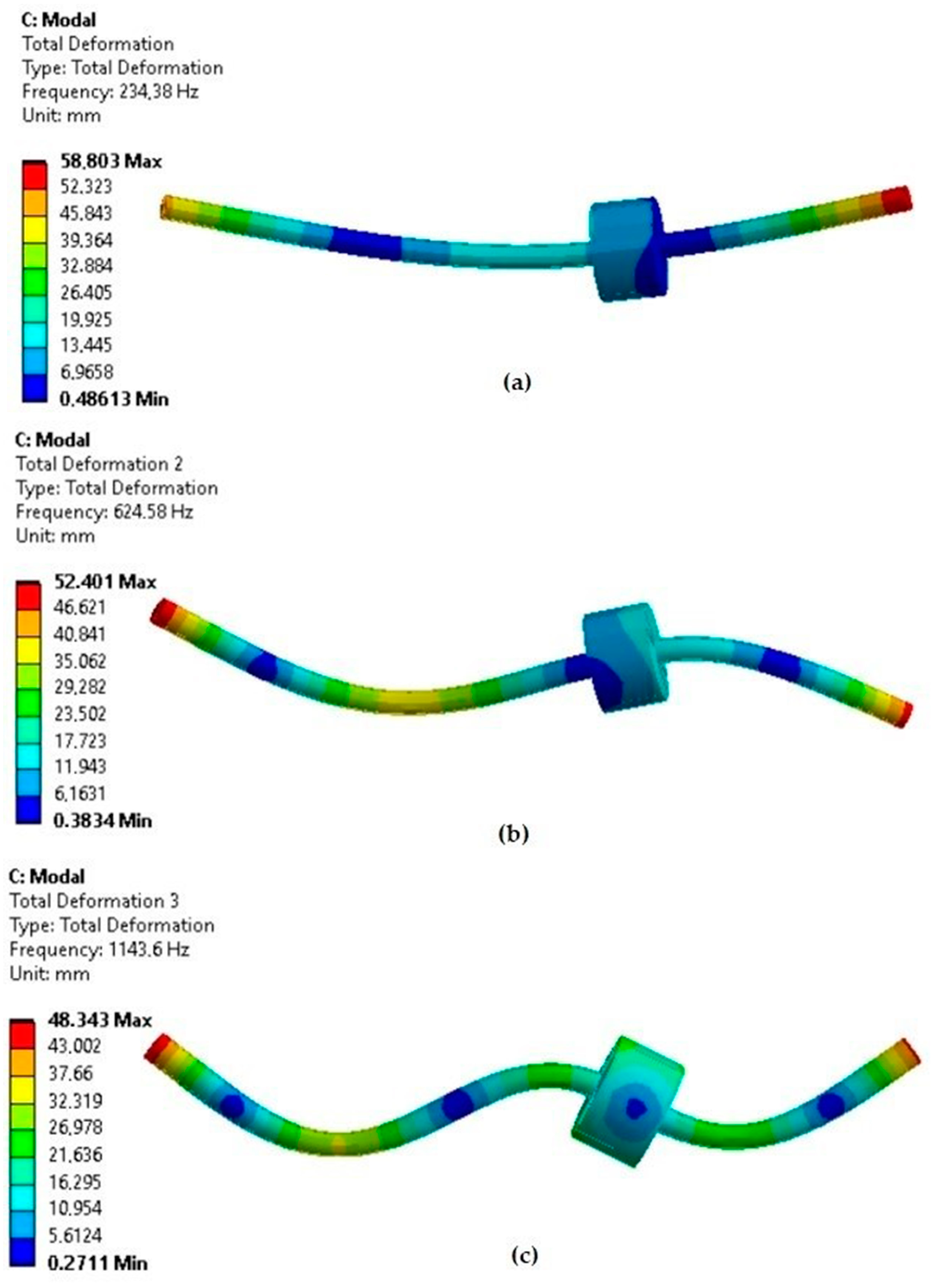
| [Hz] | Exact values in this work | 233.244 | 623.444 | 1139.727 | 2176.085 |
| FEM results in this work | 234.38 | 624.58 | 1143.6 | 2123.6 | |
| Reference [14] | 233.22 | 623.41 | 1139.76 | 2176.01 |
| 0 | 0 | This work [22] | 4.7300 | 7.8532 | 10.9956 | 14.1372 | 17.2788 |
| 4.7300 | 7.8532 | 10.9956 | 14.1372 | 17.2788 | |||
| 0 | 0.5 | This work [22] | 4.1281 | 7.1898 | 10.2985 | 13.4210 | 16.5503 |
| 4.1281 | 7.1898 | 10.2985 | 13.4210 | 16.5503 | |||
| 0 | 2 | This work [22] | 3.9887 | 7.1025 | 10.2340 | 13.3701 | 16.5083 |
| 3.9887 | 7.1025 | 10.2340 | 13.3701 | 16.5083 | |||
| 1 | 0.5 | This work [22] | 3.4887 | 6.4873 | 9.5687 | 12.6773 | 15.7981 |
| 3.4887 | 6.4873 | 9.5687 | 12.6773 | 15.7981 | |||
| 1 | 2 | This work [22] | 3.1416 | 6.2832 | 9.4748 | 12.5664 | 15.7080 |
| 3.1416 | 6.2832 | 9.4748 | 12.5664 | 15.7080 |
| 0 | This work [22] | 3.9266 | 7.0686 | 10.2102 | 13.3518 | 16.4934 | |||
| 3.9266 | 7.0686 | 10.2102 | 13.3518 | 16.4934 | |||||
| 1 | This work [22] | 3.2733 | 9.3560 | 9.4749 | 12.6045 | 15.7387 | |||
| 3.2733 | 9.3560 | 9.4749 | 12.6045 | 15.7387 | |||||
| 1 | This work [22] | 3.2733 | 9.3560 | 9.4749 | 12.6045 | 15.7387 | |||
| 3.2733 | 9.3560 | 9.4749 | 12.6045 | 15.7387 | |||||
| This work [22] | 3.3417 | 6.3932 | 9.5004 | 12.6239 | 15.7543 | ||||
| 3.3417 | 6.3932 | 9.5004 | 12.6239 | 15.7542 | |||||
| 0.0 | 9.5312 | 38.3368 | 86.9889 | 159.8826 | 254.7255 |
| 0.2 | 0.5324 | 9.5694 | 86.9938 | 159.8850 | 254.7270 |
| 0.5 | 0.8414 | 9.6265 | 38.3656 | 87.0010 | 159.8887 |
| 1.0 | 1.1888 | 9.7209 | 38.3945 | 87.0132 | 159.8948 |
| 4.0 | 2.3647 | 10.2680 | 38.5677 | 87.0861 | 159.9314 |
| 40 | 7.0436 | 15.2901 | 40.6387 | 87.9692 | 160.3740 |
| 0.000 | 23.0989 | 61.4644 | 123.1367 | 206.9218 | 316.5472 |
| 0.001 | 23.0011 | 61.2063 | 122.6352 | 206.0671 | 315.1631 |
| 0.005 | 22.6242 | 60.2273 | 120.7634 | 202.9266 | 310.1725 |
| 0.010 | 22.1823 | 59.1120 | 118.6908 | 199.5410 | 304.9545 |
| 0.100 | 17.41213 | 49.0645 | 102.7492 | 176.7382 | 274.1186 |
| 1.000 | 10.7246 | 39.8444 | 91.8901 | 164.1757 | 259.9646 |
| 2.000 | 9.7652 | 38.9051 | 90.9567 | 163.1918 | 258.9270 |
| ) | ) | |||||
|---|---|---|---|---|---|---|
| 0.0 (0.0) | 0.0 (0.0) | Exact FEM | 228.6947 | 618.1035 | 1167.0979 | 2082.1333 |
| 227.9798 | 612.7171 | 1154.6921 | 2026.2247 | |||
| 1503.892 (0.2) | 541.402 (0.2) | Exact FEM | 235.8138 | 626.0366 | 1174.5282 | 2089.5989 |
| 235.0627 | 620.5318 | 1161.9912 | 2033.4418 | |||
| 3759.73 (0.5) | 1353.505 (0.5) | Exact FEM | 245.4496 | 637.2379 | 1185.2174 | 2100.4596 |
| 244.6618 | 631.5668 | 1172.4953 | 2043.9357 | |||
| 7519.46 (1.0) | 2707.01 (1.0) | Exact FEM | 259.2636 | 654.2485 | 1201.9007 | 2117.7039 |
| 258.4149 | 648.3079 | 1188.8752 | 2060.5783 | |||
| 30,077.84 (4.0) | 10,828.04 (4.0) | Exact FEM | 309.7872 | 726.4879 | 1279.0437 | 2202.4609 |
| 308.6328 | 719.1648 | 1264.3755 | 2142.0185 | |||
| 300,778.4 (40) | 108,280.4 (40) | Exact FEM | 407.8250 | 891.7241 | 1491.0766 | 2482.5238 |
| 405.9734 | 879.8590 | 1469.8359 | 2271.3417 |
| Presentation | Figure | Plots |
|---|---|---|
| 1 | Figure 6 | |
| 2 | Figure 7 | |
| 3 | Figure 8 | |
| 4 | Figure 9 | |
| 5 | Figure 10 | |
| 6 | Figure 11 |
| diff % | diff % | diff % | ||||
|---|---|---|---|---|---|---|
| 0.01 | 0.12909 | 0.00 | 3.10968 | 0.00 | 22.15887 | 0.00 |
| 0.05 | 0.28860 | 123.57 | 3.13779 | 0.90 | 22.16333 | 0.02 |
| 0.1 | 0.40803 | 216.08 | 3.17257 | 2.02 | 22.16891 | 0.05 |
| 0.2 | 0.57674 | 346.77 | 3.24101 | 4.22 | 22.18007 | 0.10 |
| 0.5 | 0.91047 | 605.30 | 3.43805 | 10.56 | 22.21355 | 0.25 |
| 0.6 | 0.99684 | 672.21 | 3.50124 | 12.59 | 22.22472 | 0.30 |
| 0.8 | 1.14985 | 790.74 | 3.62427 | 16.55 | 22.24705 | 0.40 |
| 1 | 1.28422 | 894.83 | 3.74320 | 20.37 | 22.26938 | 0.50 |
| 2 | 1.80675 | --- | 4.28790 | --- | 22.38112 | --- |
| 4 | 2.52896 | --- | 5.20595 | --- | 22.60488 | --- |
| 10 | 3.87968 | --- | 7.27881 | --- | 23.27715 | --- |
| 20 | 5.22812 | --- | 9.75792 | --- | 24.39430 | --- |
| 40 | 6.76651 | --- | 13.27991 | --- | 26.58144 | --- |
| 0.1 | 1.14331 | 2.46153 | 19.94128 |
| 0.4 | 1.14571 | 3.26781 | 20.77100 |
| 1.0 | 1.14753 | 4.29175 | 22.17412 |
| 2.0 | 1.14894 | 5.30581 | 23.97465 |
| 10 | 1.15153 | 7.58801 | 29.83247 |
| 40 | 1.15245 | 8.57408 | 33.38169 |
| 400 | 1.15278 | 8.96146 | 34.99618 |
| 4000 | 1.15282 | 9.00333 | 35.17895 |
Disclaimer/Publisher’s Note: The statements, opinions and data contained in all publications are solely those of the individual author(s) and contributor(s) and not of MDPI and/or the editor(s). MDPI and/or the editor(s) disclaim responsibility for any injury to people or property resulting from any ideas, methods, instructions or products referred to in the content. |
© 2025 by the author. Licensee MDPI, Basel, Switzerland. This article is an open access article distributed under the terms and conditions of the Creative Commons Attribution (CC BY) license (https://creativecommons.org/licenses/by/4.0/).
Share and Cite
Kostekci, F. An Analytical Solution for Natural Frequencies of Elastically Supported Stepped Beams with Rigid Segments. Appl. Mech. 2025, 6, 12. https://doi.org/10.3390/applmech6010012
Kostekci F. An Analytical Solution for Natural Frequencies of Elastically Supported Stepped Beams with Rigid Segments. Applied Mechanics. 2025; 6(1):12. https://doi.org/10.3390/applmech6010012
Chicago/Turabian StyleKostekci, Ferid. 2025. "An Analytical Solution for Natural Frequencies of Elastically Supported Stepped Beams with Rigid Segments" Applied Mechanics 6, no. 1: 12. https://doi.org/10.3390/applmech6010012
APA StyleKostekci, F. (2025). An Analytical Solution for Natural Frequencies of Elastically Supported Stepped Beams with Rigid Segments. Applied Mechanics, 6(1), 12. https://doi.org/10.3390/applmech6010012