On Solving Nonlinear Elasticity Problems Using a Boundary-Elements-Based Solution Method

Abstract
:1. Introduction
2. Governing Equations and Solution Method
2.1. Basic Definitions and Governing Equations
2.2. Solution Method Using the LPI-BEM
- Particular Integral:
| 1/ Initialisation: material data, loading steps, etc. |
2/ Conventional BEM phase
|
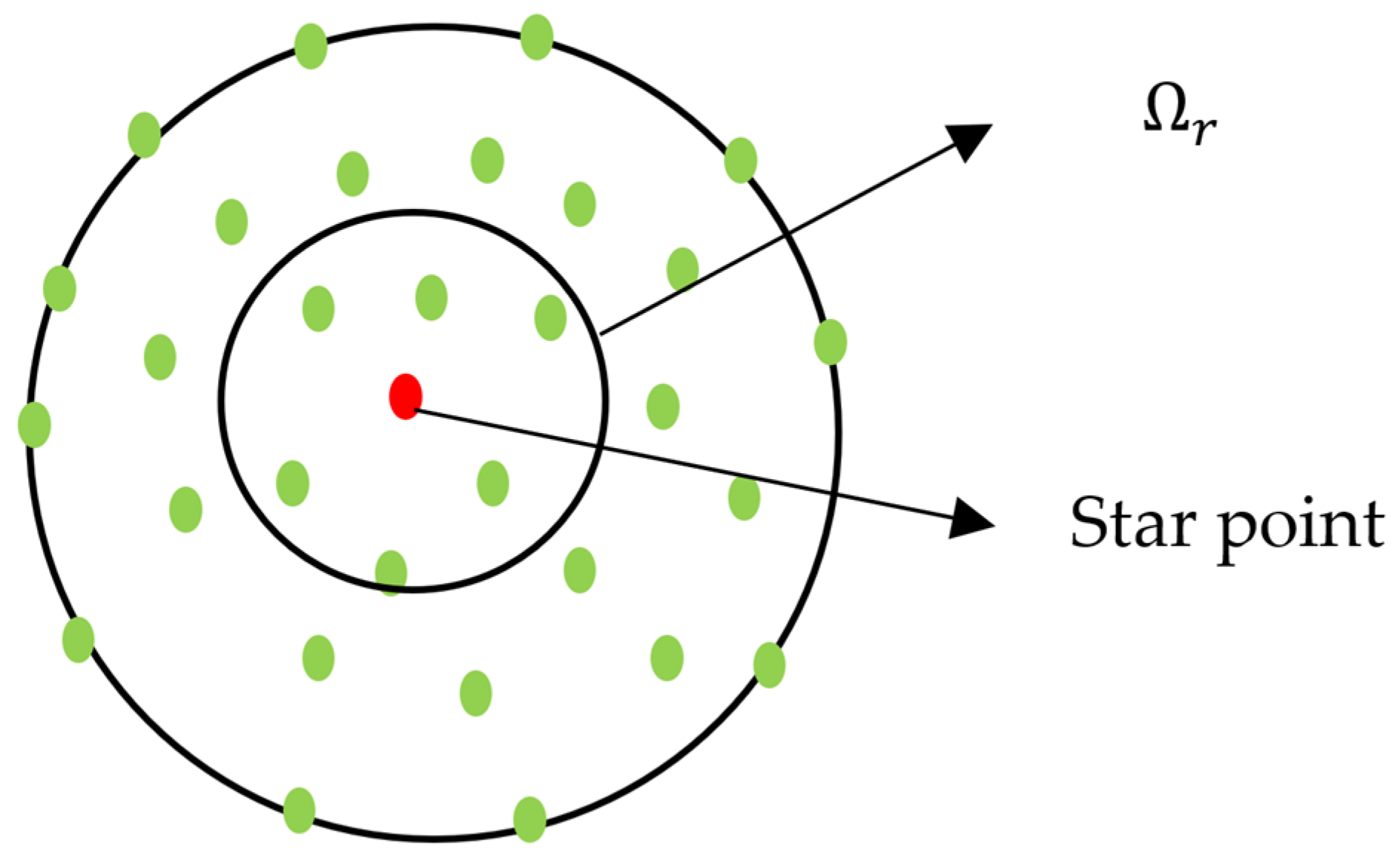
3/ Radial point interpolation phase
|
4/ Apply boundary conditions:
|
| 5/ Nonlinear solution phase Do until the final load increment
|
| 6/ End program |
3. Numerical Examples
3.1. Material Models
- Isotropic Saint Venant–Kirchhoff Model
- Isotropic Neo–Hookean Model
- Isotropic Mooney–Rivlin Model
- The Transversely Isotropic Saint Venant–Kirchhoff Model
- Neo–Hookean Transversely Isotropic Model
3.2. Case of Uni-Axial Loading
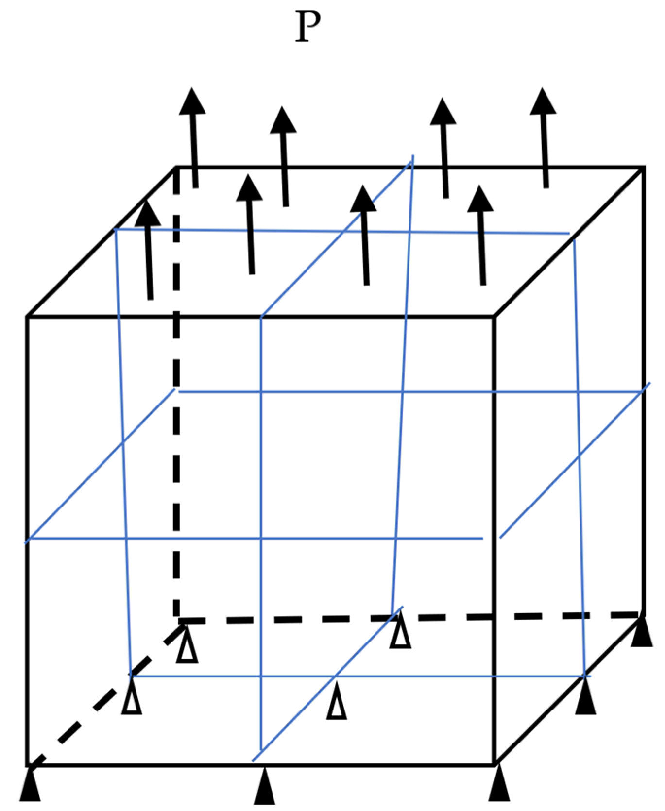
3.2.1. Unit Cube under Tension
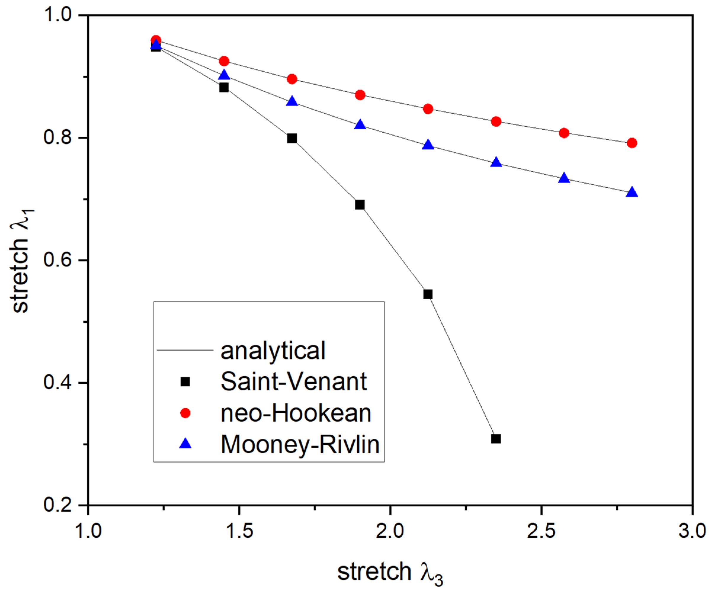
- Saint Venant–Kirchhoff Solid:
- Neo–Hookean Solid:
- Mooney–Rivlin Solid:
- Transversely Isotropic Saint Venant–Kirchhoff Solid:
- Transversely Isotropic Neo–Hookean Solid:
3.2.2. Cases of a Cylindrical Specimen under Uniaxial Loading
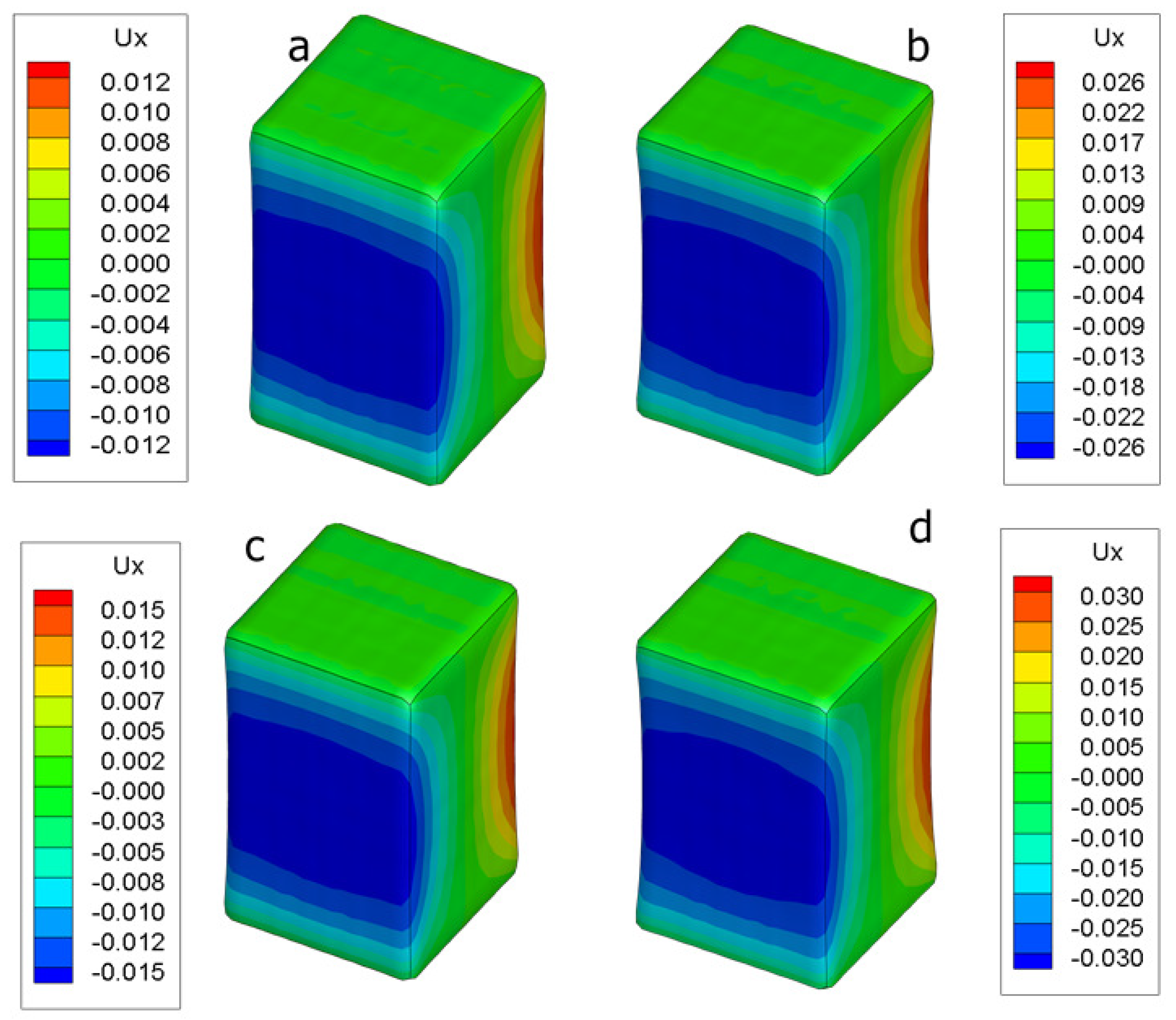
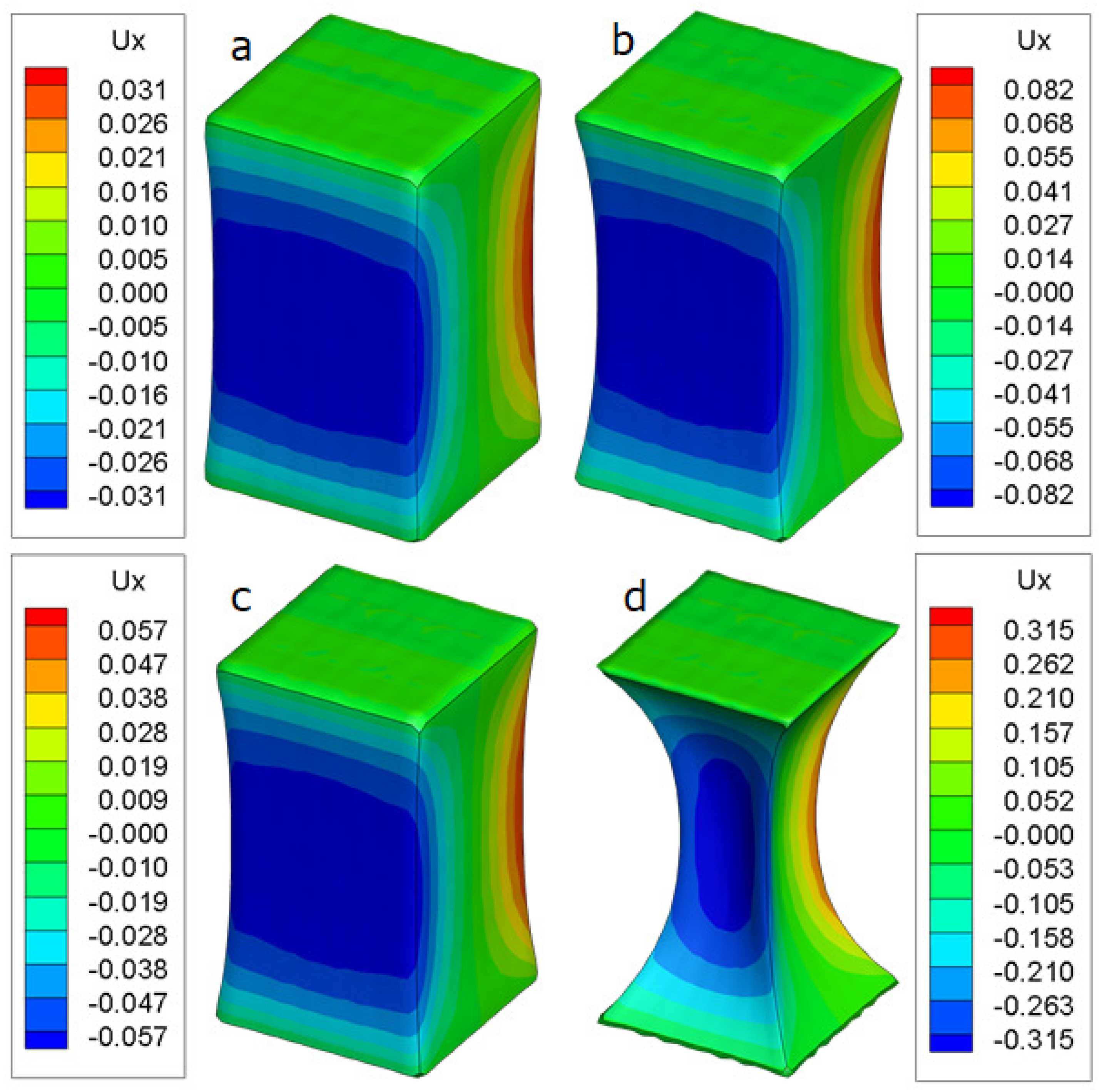
3.3. Simple Shear of a Cubic Specimen
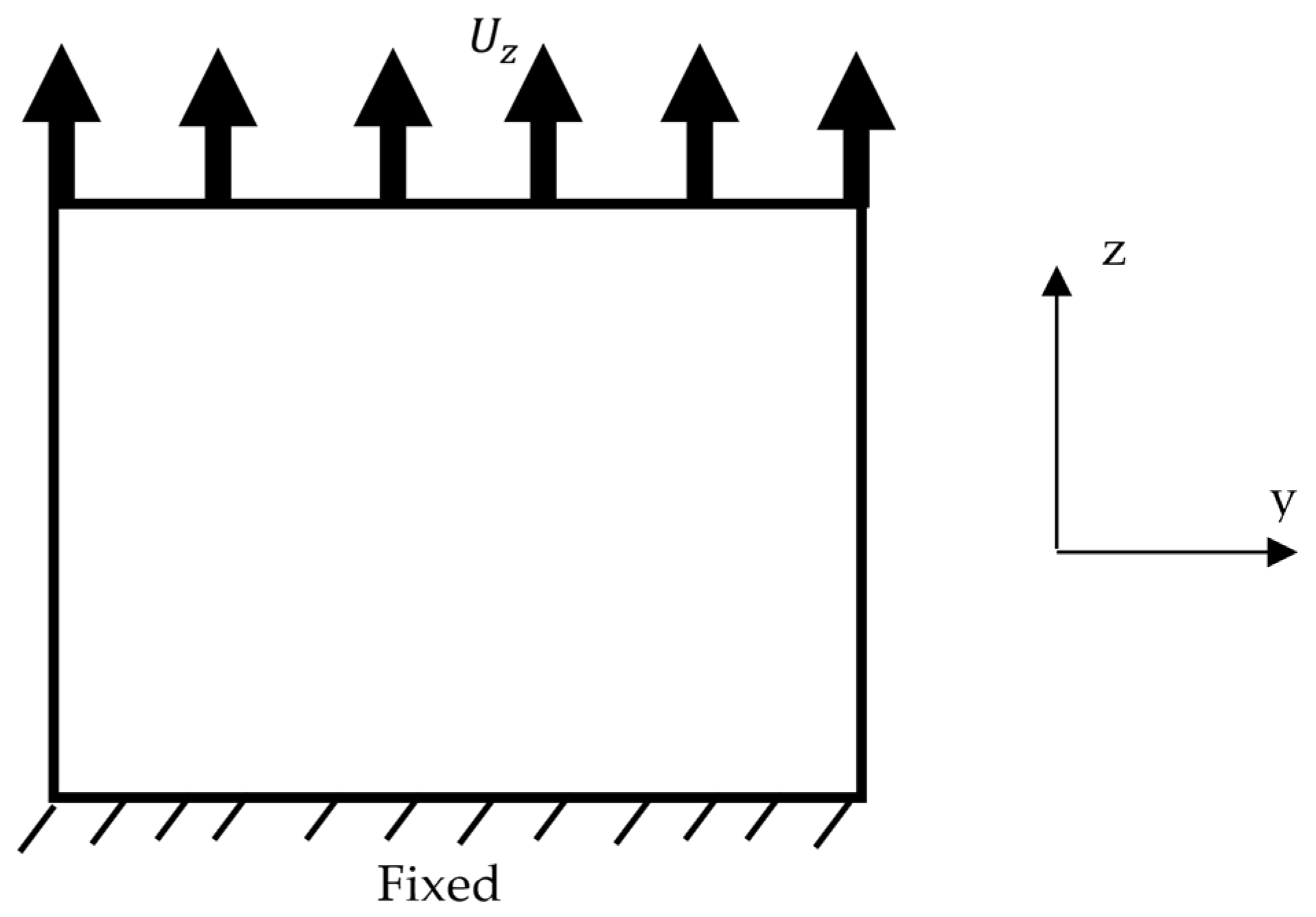
3.4. Constrained Tension of a Cubic Specimen
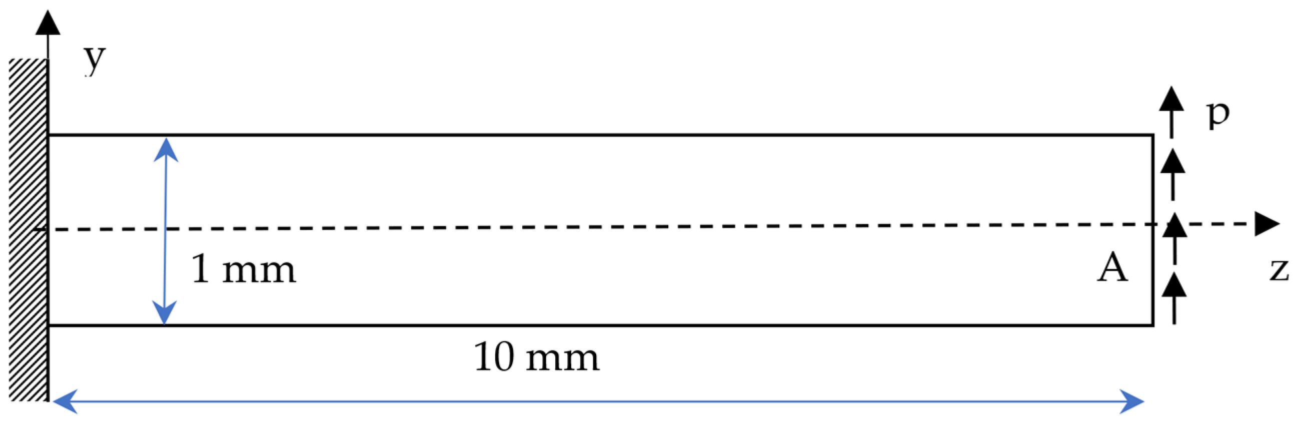
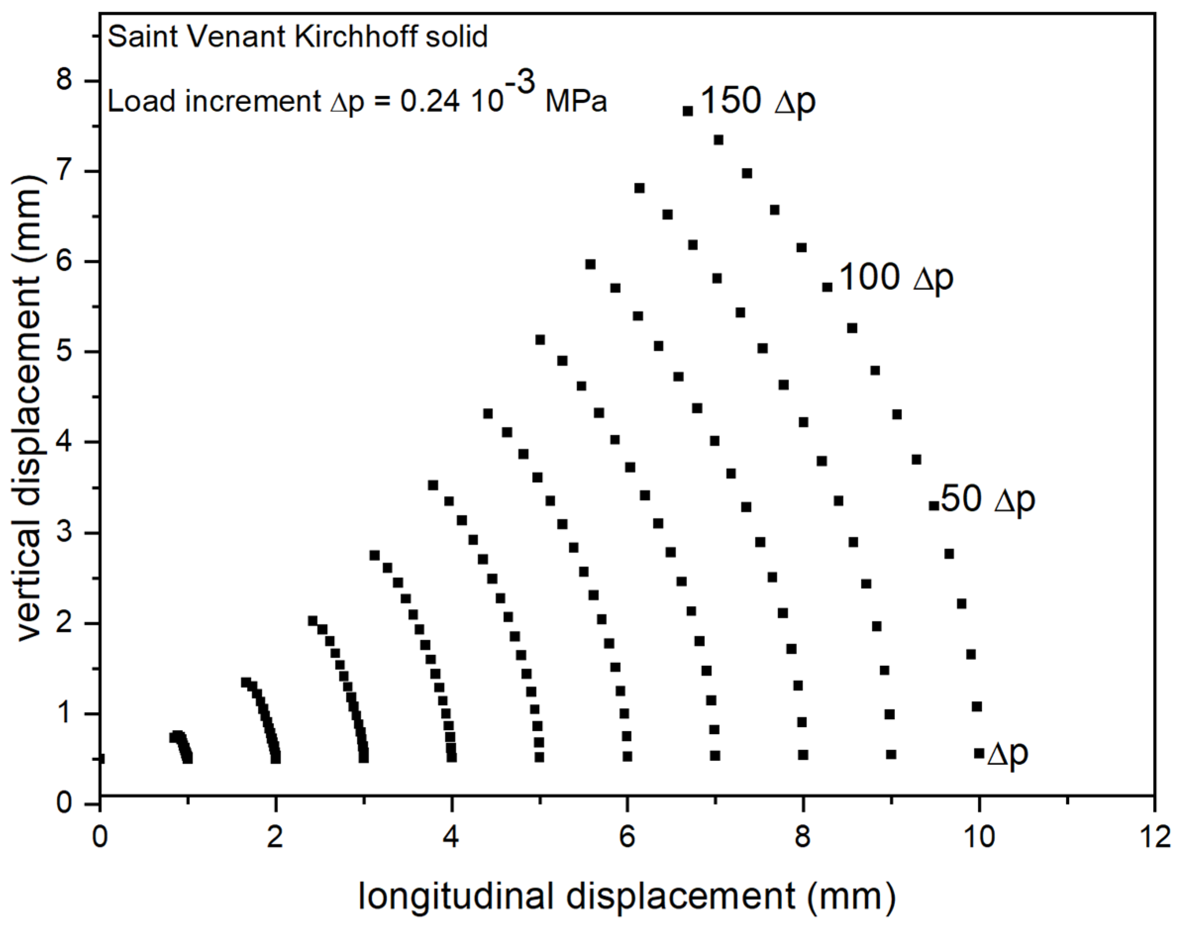
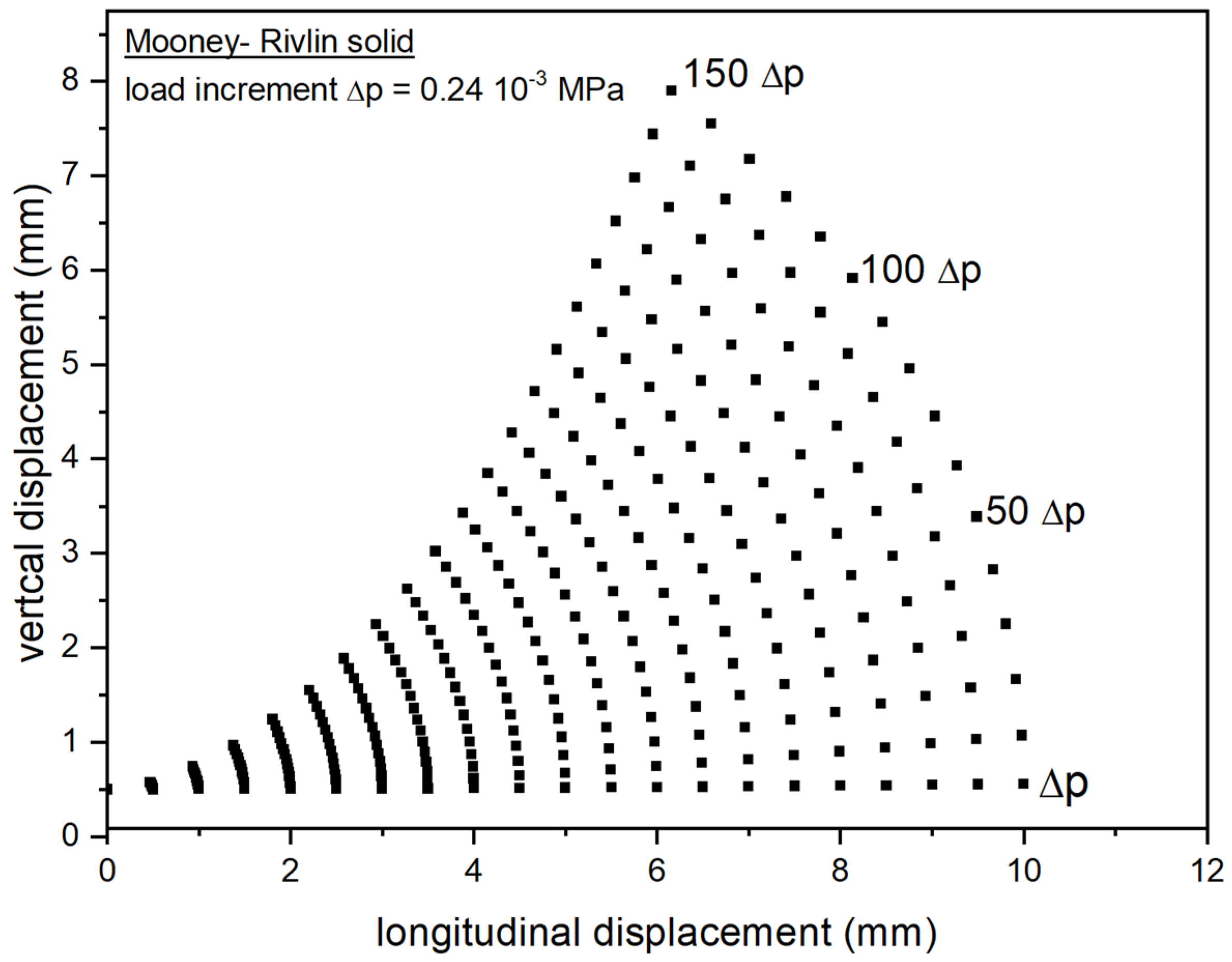
3.5. Bending of a Prismatic Bar
4. Conclusions
Author Contributions
Funding
Data Availability Statement
Acknowledgments
Conflicts of Interest
References
- Balas, J.; Sladek, J.; Sladek, V. Stress Analysis by Boundary Element Method; Elsevier: Berlin/Heilderberg, Germany, 1989. [Google Scholar]
- Bonnet, M. Boundary Integral Equation Methods for Solids and Fluids; John Wiley & Sons: New York, NY, USA, 1999; Available online: http://books.google.fr/books?id=3FBjQgAACAAJ (accessed on 20 October 2023).
- Brebbia, C.A.; Dominguez, J. Boundary Elements: An Introductory Course, Computational Mechanics Publications; WIT Press: Southampton, UK, 1992; Available online: http://books.google.fr/books?id=YBElJxdldHYC (accessed on 20 October 2023).
- Foerster, A.; Kuhn, G. A field boundary element formulation for material nonlinear problems at finite strains. Int. J. Solids Struct. 1994, 31, 1777–1792. [Google Scholar] [CrossRef]
- Al-Gahtani, H.J.; Altiero, N.J. Application of the boundary element method to rubber-like elasticity. Appl. Math. Model. 1996, 20, 654–661. [Google Scholar] [CrossRef]
- Prieto, I.; Ibán, A.L.; Garrido, J.A. 2D analysis for geometrically non-linear elastic problems using the BEM. Eng. Anal. Bound. Elem. 1999, 23, 247–256. [Google Scholar] [CrossRef]
- Nardini, D.; Brebbia, C.A. A new approach to free vibration analysis using boundary elements. Appl. Math. Model. 1983, 7, 157–162. [Google Scholar] [CrossRef]
- Gao, X.-W. The radial integration method for evaluation of domain integrals with boundary-only discretization. Eng. Anal. Bound. Elem. 2002, 26, 905–916. [Google Scholar] [CrossRef]
- Chen, L.; Kassab, A.J.; Nicholson, D.W.; Chopra, M.B. Generalized boundary element method for solids exhibiting nonhomogeneities. Eng. Anal. Bound. Elem. 2001, 25, 407–422. [Google Scholar] [CrossRef]
- Ochiai, Y. Meshless large plastic deformation analysis considering with a friction coefficient by triple-reciprocity boundary element method. Int. J. CMEM 2018, 6, 989–999. [Google Scholar] [CrossRef]
- Zhu, T.; Zhang, J.-D.; Atluri, S.N. A local boundary integral equation (LBIE) method in computational mechanics, and a meshless discretization approach. Comput. Mech. 1998, 21, 223–235. [Google Scholar] [CrossRef]
- Katsikadelis, J.T.; Nerantzaki, M.S. The boundary element method for nonlinear problems. Eng. Anal. Bound. Elem. 1999, 23, 365–373. [Google Scholar] [CrossRef]
- Brun, M.; Capuani, D.; Bigoni, D. A boundary element technique for incremental, non-linear elasticity: Part I: Formulation. Comput. Methods Appl. Mech. Eng. 2003, 192, 2461–2479. [Google Scholar] [CrossRef]
- Brun, M.; Bigoni, D.; Capuani, D. A boundary element technique for incremental, non-linear elasticity: Part II: Bifurcation and shear bands. Comput. Methods Appl. Mech. Eng. 2003, 192, 2481–2499. [Google Scholar] [CrossRef]
- Liu, G.R. Meshfree Methods: Moving Beyond the Finite Element Method, 2nd ed.; CRC Press: Boca Raton, FL, USA, 2010. [Google Scholar]
- Belytschko, T.; Lu, Y.Y.; Gu, L. Element-free Galerkin methods. Int. J. Numer. Methods Eng. 1994, 37, 2. [Google Scholar] [CrossRef]
- Chen, J.-S.; Pan, C.; Wu, C.-T.; Liu, W.K. Reproducing Kernel Particle Methods for large deformation analysis of non-linear structures. Comput. Methods Appl. Mech. Eng. 1996, 139, 195–227. [Google Scholar] [CrossRef]
- Chen, J.-S.; Pan, C.; Wu, C.-T. Large deformation analysis of rubber based on a reproducing kernel particle method. Comput. Mech. 1997, 19, 3. [Google Scholar] [CrossRef]
- Zhang, X.; Yao, Z.; Zhang, Z. Application of MLPG in Large Deformation Analysis. Acta Mech. Sin. 2006, 22, 331–340. [Google Scholar] [CrossRef]
- Liew, K.M.; Ng, T.Y.; Wu, Y.C. Meshfree method for large deformation analysis–a reproducing kernel particle approach. Eng. Struct. 2002, 24, 543–551. [Google Scholar] [CrossRef]
- Areias, P.; Fernandes, J.L.M.; Rodrigues, H.C. Galerkin-based finite strain analysis with enriched radial basis interpolation. Comput. Methods Appl. Mech. Eng. 2022, 394, 114873. [Google Scholar] [CrossRef]
- Areias, P.; Fernandes, L.; Melicio, R. Moving least-squares in finite strain analysis with tetrahedra support. Eng. Anal. Bound. Elem. 2022, 139, 1–13. [Google Scholar] [CrossRef]
- Röthlin, M.; Klippel, H.; Wegener, K. Meshless Methods for Large Deformation Elastodynamics. arXiv 2018. [Google Scholar] [CrossRef]
- Wu, C.T.; Hu, W.; Chen, J.S. A meshfree-enriched finite element method for compressible and near-incompressible elasticity. Numer. Methods Eng. 2012, 90, 882–914. [Google Scholar] [CrossRef]
- Zhou, B.; Zhang, C.; Zhao, F. A Finite Element-Meshless Hybrid Method (FEMLHM) of Elasticity Problem and Its Applications. Mech. Solids 2023, 58, 852–871. [Google Scholar] [CrossRef]
- Yu, S.Y.; Peng, M.J.; Cheng, H.; Cheng, Y.M. The improved element-free Galerkin method for three-dimensional elastoplasticity problems. Eng. Anal. Bound. Elem. 2019, 104, 215–224. [Google Scholar] [CrossRef]
- Liu, G.R.; Gu, Y.T. A local radial point interpolation method (LRPIM) for free vibration analyses of 2-D solids. J. Sound Vib. 2001, 246, 29–46. [Google Scholar] [CrossRef]
- Liu, G.R.; Gu, Y.T. A meshfree method: Meshfree weak?strong (MWS) form method, for 2-D solids. Comput. Mech. 2003, 33, 2–14. [Google Scholar] [CrossRef]
- Lee, S.-H.; Yoon, Y.-C. Meshfree point collocation method for elasticity and crack problems. Int. J. Numer. Methods Eng. 2004, 61, 22–48. [Google Scholar] [CrossRef]
- Zheng, H.; Lai, X.; Hong, A.; Wei, X. A Novel RBF Collocation Method Using Fictitious Centre Nodes for Elasticity Problems. Mathematics 2022, 10, 3711. [Google Scholar] [CrossRef]
- Njiwa, R.K. Isotropic-BEM coupled with a local point interpolation method for the solution of 3D-anisotropic elasticity problems. Eng. Anal. Bound. Elem. 2011, 35, 4. [Google Scholar] [CrossRef]
- Njiwa, R.K.; Pierson, G.; Voignier, A. Coupling BEM and the Local Point Interpolation for the Solution of Anisotropic Elastic Nonlinear, Multi-Physics and Multi-Fields Problems. Int. J. Comput. Methods 2019, 17, 1950067. [Google Scholar] [CrossRef]
- Thurieau, N.; Njiwa, R.K.; Taghite, M. A simple solution procedure to 3D-piezoelectric problems: Isotropic BEM coupled with a point collocation method. Eng. Anal. Bound. Elem. 2012, 36, 11. [Google Scholar] [CrossRef]
- Pierson, G.; Taghite, M.; Bravetti, P.; Njiwa, R.K. Spherical Indentation of a Micropolar Solid: A Numerical Investigation Using the Local Point Interpolation–Boundary Element Method. Appl. Mech. 2021, 2, 581–590. [Google Scholar] [CrossRef]
- Ciarlet, P.G. Mathematical Elasticity: Three-Dimensional Elasticity; Society for Industrial & Applied Mathematics (SIAM): Philadelphia, PA, USA, 2021. [Google Scholar] [CrossRef]
- Maugin, G.A. On canonical equations of continuum thermomechanics. Mech. Res. Commun. 2006, 33, 705–710. [Google Scholar] [CrossRef]
- Park, K.-H.; Banerjee, P.K. Two- and three-dimensional transient thermoelastic analysis by BEM via particular integrals. Int. J. Solids Struct. 2002, 39, 2871–2892. [Google Scholar] [CrossRef]
- Karami, G.; Derakhshan, D. A field boundary element for large deformation analysis of hyperelastic problems. Sci. Iran. 2001, 2, 110–122. [Google Scholar]
- Yu, Z. On the global convergence of a Levenberg-Marquardt method for constrained nonlinear equations. J. Appl. Math. Comput. 2004, 16, 183–194. [Google Scholar] [CrossRef]
- Hu, D.; Sun, Z. The Meshless Local Petrov-Galerkin Method for Large Deformation Analysis of Hyperelastic Materials. ISRN Mech. Eng. 2011, 2011, 967512. [Google Scholar] [CrossRef]
- Kompiš, V.; Toma, M.; Žmindák, M.; Handrik, M. Use of Trefftz functions in non-linear BEM/FEM. Comput. Struct. 2004, 82, 2351–2360. [Google Scholar] [CrossRef]
- Gu, Y.T.; Wang, Q.X.; Lam, K.Y. A meshless local Kriging method for large deformation analyses. Comput. Methods Appl. Mech. Eng. 2007, 196, 1673–1684. [Google Scholar] [CrossRef]
- Crisfield, M.A. Non-Linear Finite Element Analysis of Solids and Structures, 2nd ed.; John Wiley & Sons, Ltd.: Chichester, NY, USA, 1991. [Google Scholar]
- Hu, D.A.; Long, S.Y.; Han, X.; Li, G.Y. A meshless local Petrov–Galerkin method for large deformation contact analysis of elastomers. Eng. Anal. Bound. Elem. 2007, 31, 657–666. [Google Scholar] [CrossRef]
- Bonet, J.; Burton, A.J. A simple orthotropic, transversely isotropic hyperelastic constitutive equation for large strain computations. Comput. Methods Appl. Mech. Eng. 1998, 162, 151–164. [Google Scholar] [CrossRef]
- Kulkarni, M.; Carnahan, D.; Kulkarni, K.; Qian, D.; Abot, J.L. Elastic response of a carbon nanotube fiber reinforced polymeric composite: A numerical and experimental study. Compos. Part B Eng. 2010, 41, 414–421. [Google Scholar] [CrossRef]
- Destrade, M.; Murphy, J.; Saccomandi, G. Simple shear is not so simple. Int. J. Non-Linear Mech. 2012, 47, 210–214. [Google Scholar] [CrossRef]
- Mihai, L.A.; Goriely, A. Numerical simulation of shear and the Poynting effects by the finite element method: An application of the generalised empirical inequalities in non-linear elasticity. Int. J. Non-Linear Mech. 2013, 49, 1–14. [Google Scholar] [CrossRef]
- Foroutan, M.; Dalayeli, H.; Sadeghian, M. Simulation of Large Deformations of Rubbers by the RKPM Method. Int. J. Math. Comput. Phys. Electr. Comput. Eng. 2007, 1, 136–141. [Google Scholar]


| Material | |||||
|---|---|---|---|---|---|
| Set 1 | 7.22 | 23 | 0.14 | 0.08789 | 4.20 |
| Set 2 | 4.71 | 13.7 | 0.14 | 0.0997 | 1.49 |
| SVK_T1 | SVK_T2 | NH_T1 | NH_T2 | |||||
|---|---|---|---|---|---|---|---|---|
| Anal | Num | Anal | Num | Anal | Num | Anal | Num | |
| 1.225 | 0.9273 | 0.92726 | 0.92456 | 0.9242 | 0.9359 | 0.93592 | 0.93356 | 0.93356 |
| 1.45 | 0.8315 | 0.83144 | 0.82479 | 0.8226 | 0.8682 | 0.868178 | 0.8632 | 0.86324 |
| 1.675 | 0.7032 | 0.70318 | 0.6902 | 0.6884 | 0.7952 | 0.79524 | 0.7874 | 0.78746 |
| 1.9 | 0.5189 | 0.51884 | 0.4931 | 0.4894 | 0.7162 | 0.716116 | 0.7054 | 0.7054 |
| Saint Venant–Kirchhoff | Neo–Hookean | SVK_T1 | NH_T1 | |||||
|---|---|---|---|---|---|---|---|---|
| −1.8571 | −3.24745 | −3.09577 | −4.018277 | |||||
| Anal | Num | Anal | Num | Anal | Num | Anal | Num | |
| 0.775 | 0.775 | 0.775 | 0.775 | 0.775 | 0.775 | 0.775 | 0.7625 | |
| 1.03917 | 1.03918 | 1.0507 | 1.0507 | 1.054 | 1.05436 | 1.063 | 1.0543 | |
| −2.30175 | −8.612425 | −3.837 | −7.9176 | |||||
| Anal | Num | Anal | Num | Anal | Num | Anal | Num | |
| 0.55 | 0.6044 | 0.55 | 0.55 | 0.55 | 0.6044 | 0.55 | 0.5152 | |
| 1.0675 | 1.06159 | 1.1179 | 1.1179 | 1.0933 | 1.08523 | 1.1298 | 1.1238 | |
| Model | ||||||||
|---|---|---|---|---|---|---|---|---|
| Stress component | Saint–Venant | Neo–Hookean | Mooney–Rivlin | SV_T1 | SV_T2 | NH_T1 | NH_T2 | |
| 0.755 | 0.3125 | 0.1042 | 0.436 | 0.2854 | 0.1979 | 0.1291 | ||
| 0.417 | 0 | −0.208 | 0.238 | 0.1563 | 0 | 0 | ||
| 0.104 | 0 | 0.1042 | 0.078 | 0.0532 | 0.0377 | 0.0260 | ||
| 1.354 | 1.25 | 1.25 | 0.792 | 0.5164 | 0.7917 | 0.5164 | ||
Disclaimer/Publisher’s Note: The statements, opinions and data contained in all publications are solely those of the individual author(s) and contributor(s) and not of MDPI and/or the editor(s). MDPI and/or the editor(s) disclaim responsibility for any injury to people or property resulting from any ideas, methods, instructions or products referred to in the content. |
© 2023 by the authors. Licensee MDPI, Basel, Switzerland. This article is an open access article distributed under the terms and conditions of the Creative Commons Attribution (CC BY) license (https://creativecommons.org/licenses/by/4.0/).
Share and Cite
Korbeogo, A.R.; Bonzi, B.K.; Kouitat Njiwa, R. On Solving Nonlinear Elasticity Problems Using a Boundary-Elements-Based Solution Method. Appl. Mech. 2023, 4, 1240-1259. https://doi.org/10.3390/applmech4040064
Korbeogo AR, Bonzi BK, Kouitat Njiwa R. On Solving Nonlinear Elasticity Problems Using a Boundary-Elements-Based Solution Method. Applied Mechanics. 2023; 4(4):1240-1259. https://doi.org/10.3390/applmech4040064
Chicago/Turabian StyleKorbeogo, Aly Rachid, Bernard Kaka Bonzi, and Richard Kouitat Njiwa. 2023. "On Solving Nonlinear Elasticity Problems Using a Boundary-Elements-Based Solution Method" Applied Mechanics 4, no. 4: 1240-1259. https://doi.org/10.3390/applmech4040064
APA StyleKorbeogo, A. R., Bonzi, B. K., & Kouitat Njiwa, R. (2023). On Solving Nonlinear Elasticity Problems Using a Boundary-Elements-Based Solution Method. Applied Mechanics, 4(4), 1240-1259. https://doi.org/10.3390/applmech4040064