Article

An Intuitive Derivation of Beam Models of Arbitrary Order

Shinc Inc., 505 Glenlake Avenue, Toronto, ON M6P 1G9, Canada
Appl. Mech. 2023, 4(1), 109-140; https://doi.org/10.3390/applmech4010008
Submission received: 14 December 2022 / Revised: 12 January 2023 / Accepted: 23 January 2023 / Published: 28 January 2023

Abstract

:
This article presents a new beam model that employs a recursive derivation procedure that enables the user to set the order of the governing differential equations as an input parameter, without the need for ad hoc assumptions or methodologies. This article employs a novel system of kinematic variables, section constants, and section functions that facilitate the development of higher-order beam models that retain a clear philosophical link to classical beam models such as Euler–Bernoulli beam theory and Timoshenko beam theory. The present beam model is a type of equivalent single layer beam model, wherein section constants are used to model the global stiffness characteristics of the beam, and section functions are used to recover sectional fields of displacements, strains, and stresses. The present beam model is solved for several example beams, and the results are compared to the results of finite element analyses. It is shown that the present beam model can accurately predict the deformed shapes and stress fields of each of the example beams. This article also reveals an interesting peculiarity of the elastic potential energy that pertains to any unidimensional beam model that is governed by differential equations that are of finite order.

1. Introduction

While continual improvements to accessible computing power have corresponded to ongoing increases in the prevalence of the finite element method and other computational modeling techniques, the academic and industrial sectors continue to extensively utilize classical unidimensional beam models such as Euler–Bernoulli beam theory and Timoshenko beam theory [1,2].
In Euler–Bernoulli beam theory, the internal bending moments produce curvatures that are dependent upon the flexural (bending) stiffness of the beam; these curvatures are then successively integrated in order to determine the transverse deflections of the beam. Timoshenko beam theory [1,2], which is a type of first-order shear deformation theory, improves upon Euler–Bernoulli beam theory by accounting for additional transverse compliance that is caused by shear deformations. First-order shear deformation theories typically model transverse deflections as the super-position of deflections that are caused by bending and deflections that are caused by shear. Such theories are dependent upon information pertaining to the material properties of the beam, the geometric dimensions of the beam, and derived section constants that represent the mechanical characteristics of the beam.
While the finite element method and other computational structural modeling techniques offer high fidelity solutions to an extremely diverse range of structural analysis problems, such techniques can be likened to a well-instrumented experimental test: a great deal of data is provided, but the interpretation of these data is largely dependent upon the experience of the engineer. Conversely, if an engineer is able to correlate experimental observations with the predictions of a beam model that is dependent upon section constants, then the aforementioned section constants may be used for subsequent analysis efforts, as well as to achieve a more comprehensive and intuitive understanding of the mechanical behaviour of the beam. For example, the section constants that are employed by Timoshenko beam theory provide valuable insight pertaining to the relationship between the flexural stiffness and the transverse shear stiffness of a beam, and an engineer may be able to improve upon the design of such a beam by imposing design changes that are known to directly influence the value of a section constant that has been deemed sub-optimal. Therefore, simple unidimensional beam models that are based upon section constants continue to offer practical benefits that are typically absent from finite element methods and other computational structural modeling techniques.
First-order shear deformation theories are unable to account for the effects of non-uniform warping, which limits the fidelity of first-order shear deformation theories [3,4,5]. Higher-order beam models endeavor to account for non-uniform warping of beams and plates [3,6,7,8], thereby overcoming the inherent limitations of first-order shear deformation theories. A beam model that employs third-order shear deformation theory is generally regarded as a type of higher-order beam model. Unfortunately, third-order shear deformation theories give inaccurate predictions for beams that have heterogeneous compositions due to the erroneous cubic warping displacement field that is assumed by such theories; this problem is particularly pronounced in the analysis of laminated composite beams and plates [9].
In order to more accurately model the warping displacement fields of laminated composite beams and plates, numerous researchers have developed so-called “layer-wise” theories, wherein the kinematics are independently defined for each lamina within a laminate, and the layer-to-layer continuity of some physical parameters is enforced [10,11]. Unfortunately, layer-wise theories tend to be far more analytically complex and computationally expensive than classical beam models.
Some researchers have developed so-called “equivalent single layer” beam models [12], which endeavor to overcome the relatively high computational cost of layer-wise theories. A comprehensive literature review of such equivalent single layer beam models is provided in Ref. [13]. So-called “zigzag” models are a specialized type of equivalent single layer beam model, wherein the sectional warping displacement fields of laminated composite beams and plates are approximated by piecewise linear functions [10,14,15] or by piecewise polynomial functions [16].
The so-called “Carrera Unified Formulation” (CUF) [17,18,19,20,21] is a framework for the development of structural analysis and stress analysis models wherein the order of the displacement field is stipulated as a solution control parameter. With the selection of appropriate solution control parameters, CUF beam models may be configured to mimic the behaviour of Euler–Bernoulli beam theory, Timoshenko beam theory, or higher-order beam models. Practically speaking, a higher-order CUF beam model may serve as a computationally efficient alternative to a three-dimensional finite element analysis. The CUF has been used for the development of both layer-wise beam models and equivalent single layer beam models [22,23].
The present author has previously contributed to the development of another higher-order beam model [5]. In one section of Ref. [5], the authors of Ref. [5] suggest that it may be possible to extend their derivation to facilitate the development of beam models of arbitrary order; however, the present author no longer believes that the work-energy balance that is assumed in Ref. [5] would be conducive for the development of beam models of arbitrary order. Furthermore, the beam model that is presented in Ref. [5] gives some erroneous stress predictions for beams that exhibit large rates of change of sectional warping along their longitudinal axes; the present author now believes that such erroneous stress predictions are caused by the work-energy balance that is assumed in Ref. [5].
With the increasing prevalence of laminated composite materials, engineers are often faced with design problems pertaining to beams that exhibit non-trivial transverse shear compliance as well as non-trivial resistance to non-uniform warping. The mechanical response of such beams cannot be accurately predicted by first-order shear deformation theories [5]. Therefore, there continues to exist a need for higher-order unidimensional beam models that can be confidently implemented by industry engineers who are accustomed to the use of classical beam models.
Most higher-order beam models are derived and presented in a manner that has been formulated to account for a comprehensive range of mechanical phenomena. Consequently, most state-of-the-art literature on higher-order beam models employs derivations that bare little resemblance to the familiar derivations of Euler–Bernoulli beam theory and Timoshenko beam theory. While researchers who frequently review the relevant state-of-the-art literature may have little difficulty navigating any new research on a novel higher-order beam model, an engineer wishing to venture into the field of higher-order beam models for the first time would be faced with a very difficult challenge. Consequently, the use of higher-order beam models is often limited to academic researchers who focus much of their time on the development and study of such higher-order beam models.
In the present article, a new unidimensional beam model is proposed. The present beam model employs a recursive derivation procedure that enables the user to set the order of the governing differential equations as an input parameter, without the need for ad hoc assumptions or methodologies. The present article employs a novel system of kinematic variables, section constants, and section functions that facilitate the development of higher-order beam models that retain a clear philosophical link to classical beam models such as Euler–Bernoulli beam theory and Timoshenko beam theory. For example, the present beam model is predicated on the assumption that a nominal sectional plane can be fitted through the deformed shape of each section of a deformed beam; the translations and rotations of each nominal sectional plane of the beam are included among the kinematic variables of the present beam model. Therefore, the nominal sectional planes that are discussed herein can be likened to the plane sections that are assumed to exist in first-order shear deformation theories. In essence, the present beam model is a type of equivalent single layer beam model, wherein section constants are used to model the global stiffness and compliance characteristics of the beam, and section functions are used to recover sectional fields of displacements, strains, and stresses. The present beam model is well suited for analyses of laminated beams that comprise any number of laminae.
The present work does not include an exhaustive attempt to account for all of the possible loading directions, mechanical phenomena, or coupling behaviours. Instead, the present beam model has been intentionally limited to a relatively simplistic two-dimensional space; this facilitates a clear and intuitive understanding of the implications of higher-order effects, while employing a derivation that exhibits obvious philosophical similarities to classical beam theories. The present beam model is herein described in an intentionally meticulous and explicit manner in order to ensure that it can be successfully implemented by a diverse range of engineers and academic researchers, irrespective of the prior experience that these engineers and academic researchers have had with higher-order beam models.
Through the process of deriving the present beam model, this article also reveals an interesting peculiarity of the elastic potential energy that pertains to any unidimensional beam model that is governed by differential equations that are of finite order. This peculiarity is manifested as an apparent paradox that emerges during the calculation of the section constants that are employed by the present beam model.

2. Form of the Present Beam Model

2.1. General Definitions
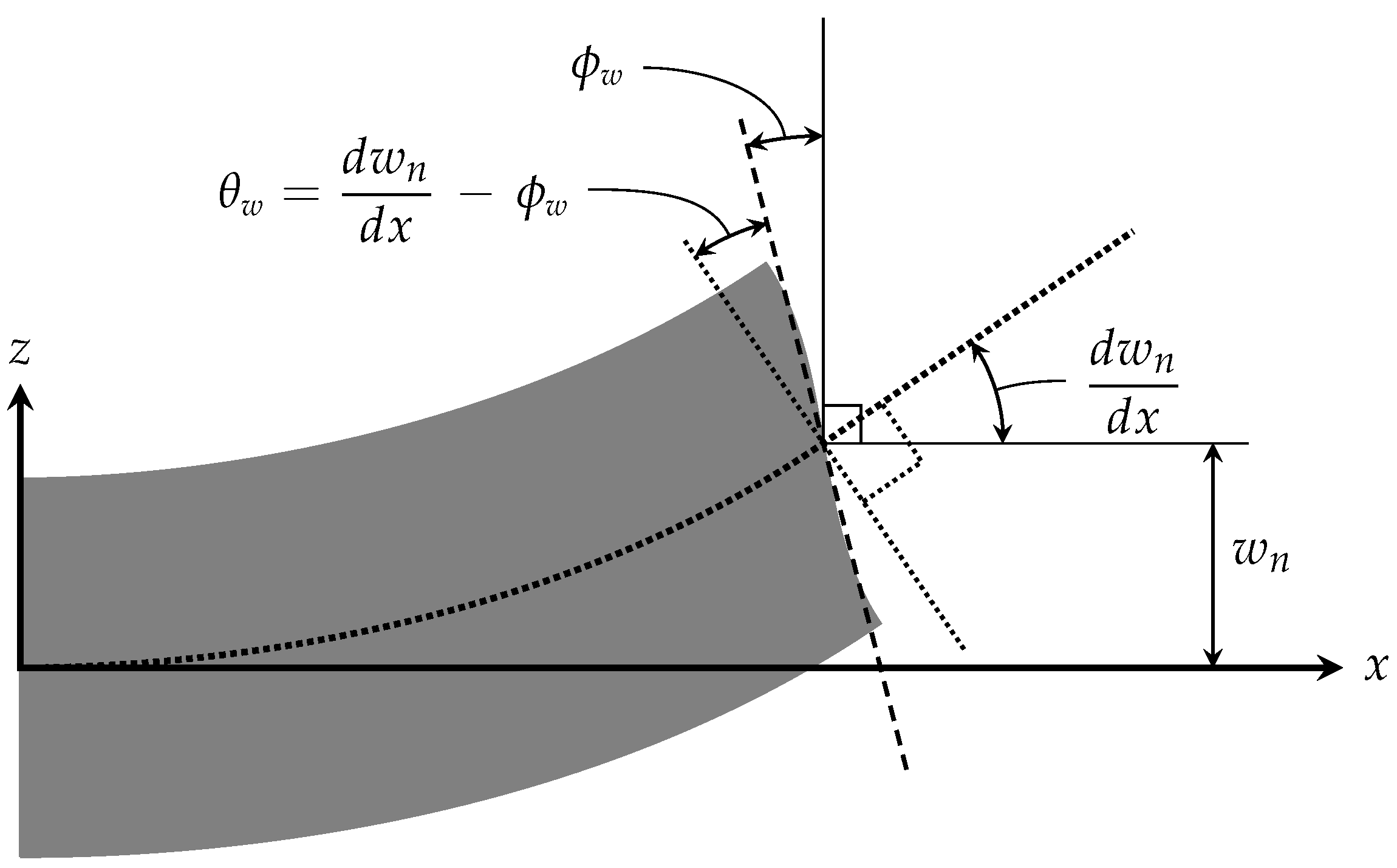
The present discussion makes use of a Cartesian coordinate system that is defined by three mutually orthogonal coordinate axes that are denoted by x, y, and z.
The term “longitudinal axis” denotes an imaginary axis that passes lengthwise through the beam. The longitudinal axis of the undeformed beam is initially parallel to the x-axis. The longitudinal axis of the beam deforms as the beam deforms; therefore, the longitudinal axis may not remain straight or parallel to the x-axis after such a deformation has occurred.
The term “longitudinal” denotes any direction that is parallel to the x-axis. The term “transverse” denotes any direction that is perpendicular to the x-axis.
The term “section” denotes a surface that would hypothetically become exposed if the beam were to be cut into two segments. When the beam does not exhibit any deformation, each section is a plane that is perpendicular to the x-axis. As the beam deforms, each section may translate and rotate relative to its initial state, and each section may deform such that it becomes non-planar.
The term “warping” herein denotes any deformation of a section that causes the section to become non-planar. The term “non-uniform warping” denotes any warping that varies along the longitudinal axis of a beam. The term “warping displacement” denotes any displacement that contributes to warping of a section.
The term “nominal sectional plane” denotes a hypothetical plane that is fitted through the deformed shape of each section of the beam. Therefore, as the beam deforms, each nominal sectional plane may translate and rotate relative to its initial state; however, each nominal sectional plane always remains planar. The specific manner in which each nominal sectional plane is fitted through the corresponding deformed section of the beam is described by the derivations that are provided herein. The present beam model does not assume that plane sections remain planar after the beam has deformed; however, the present beam model utilizes the orientation of each nominal sectional plane as a surrogate metric that helps to account for the deformation of the beam in an intuitive manner.
The term “section constant” denotes a numerical constant that represents an inherent characteristic of the material composition and geometry of a section of the beam. The term “section function” denotes a mathematical function that represents an inherent characteristic of the material composition and geometry of a section of the beam. Each section function is defined as a function of the local coordinates that are contained in the section of the beam.
The term “elevation” is used herein in reference to positions and dimensions that are measured parallel to the z-axis. Each beam section has a local z-axis that is initially parallel to the global z-axis. The origin of each local z-axis is positioned at the elevation of the bottom surface of the beam. Therefore, each z coordinate is an elevation coordinate that is measured relative to the bottom surface of the beam.
The term “local y-y axis” denotes the local flexural neutral axis that pertains to x-z curvatures. Each section of the beam has a local y-y axis. Each local y-y axis is initially parallel to the global y-axis.
The term “local z-z axis” denotes the local flexural neutral axis that pertains to x-y curvatures. Each section of the beam has a local z-z axis. Each local z-z axis is initially parallel to the global z-axis.
Some additional definitions are provided in Appendix A.

2.2. Kinematics

Figure 1 shows the deformed shape of a transversely loaded beam, and helps to illustrate some of the geometric dimensions and kinematic variables that are relevant to the present beam model.
The symbol u denotes a linear displacement that is measured parallel to the x-axis. The symbol v denotes a linear displacement that is measured parallel to the y-axis. The symbol w denotes a linear displacement that is measured parallel to the z-axis.
The symbol w n denotes the nominal value of w that corresponds to each section of the beam. At each x-coordinate, w n represents the value of w that is developed at the position of the intersection of the local y-y axis and the local z-z axis.
The symbol ϕ w denotes the angle of rotation (angular displacement) of a nominal sectional plane about its local y-y axis, measured relative to the initial orientation of the aforementioned nominal sectional plane. The value of ϕ w may vary as a function of x. The sign convention for ϕ w is defined such that a positive value of ϕ w corresponds to a rotation in the same direction as a positive value of d w n d x . Therefore, the sign convention for ϕ w does not observe the right-hand rule.
The symbol θ w denotes the total nominal shear angle that is measured within the x-z plane of the beam. The value of θ w may vary as a function of x; however, it is assumed herein that θ w is constant with respect to y and z. Since ϕ w represents a true angle of rotation of the nominal sectional plane at position x, whereas d w n d x represents a slope of the deformed longitudinal axis of the deflected beam at position x, the total nominal x-z shear angle is defined as follows:
θ w = d w n d x ϕ w .
The sign convention for θ w is defined such that a positive value of θ w corresponds to a rotation in the same direction as a positive value of d w n d x . Therefore, the sign convention for θ w does not observe the right-hand rule.
In essence, ϕ w represents the component of d w n d x that arises due to a rotation of the nominal sectional plane, whereas θ w represents the component of d w n d x that arises due to the local x-z shear deformation of the beam.
If it is assumed that d w n d x is small, then the total x-z curvature of the beam can be expressed as follows:
x - z curvature = d 2 w n d x 2 1 + d w n d x 2 3 / 2 d 2 w n d x 2 = d ϕ w d x + d θ w d x .
Integrating Equation (1) with respect to x gives the following expression for w n :
w n = ϕ w + θ w d x .
The symbol v n denotes the nominal value of v that corresponds to each section of the beam. At each x-coordinate, v n represents the value of v that is developed at the position of the intersection of the local y-y axis and the local z-z axis.
The symbol ϕ v denotes the angle of rotation (angular displacement) of a nominal sectional plane about its local z-z axis, measured relative to the initial orientation of the aforementioned nominal sectional plane.
The symbol θ v denotes the total nominal shear angle that is measured within the x-y plane of the beam. In a similar manner to Equation (1), the total nominal x-y shear angle is defined as follows:
θ v = d v n d x ϕ v .

2.3. Simplifying Assumptions

In the interest of clarity and ease of exposition, the present beam model has been developed in the context of the following simplifying assumptions:
1.
All externally applied loads act parallel to the z-axis.
2.
All externally applied concentrated moments act about axes that are parallel to the y-axis.
3.
All imposed linear displacements occur parallel to the z-axis.
4.
All imposed angular displacements (rotations) occur about axes that are parallel to the y-axis.
5.
The beam is configured such that none of the applied loadings result in the development of any non-zero values of v n , ϕ v , or θ v .
6.
The beam is configured such that none of the applied loadings result in the development of any torsional deformations of the beam.
The foregoing assumptions dictate that all transverse shear forces act parallel to the z-axis, and all moments act about axes that are parallel to the y-axis. Although the mechanical response of the beam is assumed to be symmetrical about the x-z plane, it is worth noting that the present beam model is capable of accurately modeling beams that are not symmetrical about a plane that is parallel to the x-y plane.

2.4. Governing Equations

The governing equations of the present beam model include differential equations that are herein referred to as the “governing differential equations”.
The present beam model is based upon the assumption that the displacement field within a beam can be represented by differential equations that are of infinite order. For each of the governing differential equations of the beam model, the terms of the differential equation are denoted by sequential integer values: an integer value of one denotes the term that corresponds to the lowest derivative that is present within the differential equation, and each successively greater integer value denotes a term that corresponds to a successively higher derivative that is present within the differential equation. The various terms of the governing differential equations may be represented numerically or algebraically.
The present beam model employs numerous functions, variables, and constants that are defined herein; some of these functions, variables, and constants are defined such that they correspond to a specific term of the governing differential equations of the beam model. For each function, variable, or constant that corresponds to a specific term of the governing differential equations, the aforementioned function, variable, or constant is denoted by a symbol that includes subscripted notation that appears between curly brackets; any subscripted notation that appears between curly brackets indicates which specific term of the governing differential equations corresponds to the aforementioned function, variable, or constant. For example, a function that is denoted by R { 5 } corresponds to term 5 of the governing differential equations of the beam model. Similarly, a constant that is denoted by A { j + 1 } corresponds to term j + 1 of the governing differential equations of the beam model, where j is an integer value.
The symbol u denotes the total longitudinal displacement that is developed at a point within the beam. Upon observing the simplifying assumptions that are described in Section 2.3, u can be expressed at any point within the beam, as follows:
u = j = 1 u { j } ,
where
u { j } = R { j } d ( 2 j 2 ) ϕ w d x ( 2 j 2 ) ;
u { j } is the component of the longitudinal displacement that corresponds to term j of the governing differential equations; and R { j } is a section function that corresponds to term j of the governing differential equations. At each x coordinate, Equation (6) defines the value of u { j } at any point within the section of the beam. In essence, u is the value of u that is given by Equation (5).
In cases wherein j = 1 , Equation (6) simplifies as follows:
u { 1 } = R { 1 } ϕ w .
u { 1 } describes the longitudinal displacement of each point that is contained in a nominal sectional plane of the beam; therefore, R { 1 } is a linear function of the local coordinates that are contained in the section of the beam. Conversely, for each integer value of j that is greater than one, u { j } describes a component of the longitudinal distance between each point on a deformed section of the beam and the corresponding point on the corresponding nominal sectional plane of the beam. Therefore, if the symbol u H O denotes the sum of all sectional fields of u { i } for all integer values of i that are greater than one, then u H O describes the total longitudinal distance between each point on a deformed section of the beam and the corresponding point on the corresponding nominal sectional plane of the beam.
In most cases, it is both impractical and unnecessary to define a beam using governing differential equations that are of infinite order. Therefore, it is convenient to truncate Equation (5) to a finite number of terms, as follows:
u N = j = 1 N u { j } ,
where u N is the total longitudinal displacement that is developed at a point within the beam; u { j } is the component of u N that corresponds to term j of the governing differential equations; u { j } is defined in accordance with Equation (6); and N is a finite integer value that represents the number of terms that are to be included in the truncated infinite series that represents u N . In essence, u N is the value of u that is given by Equation (8).
The symbol ε x denotes the total longitudinal normal strain that is developed at a point within the beam. At any point within the beam, ε x can be expressed by differentiating Equation (8) with respect to x, as follows:
ε x = d u N d x = j = 1 N ε { j } ,
where
ε { j } = d u { j } d x = R { j } d ( 2 j 1 ) ϕ w d x ( 2 j 1 ) ;
and ε { j } is the component of ε x that corresponds to term j of the governing differential equations.
The symbol σ x denotes the total longitudinal normal stress that is developed at a point within the beam. At any point within the beam, σ x can be expressed as follows:
σ x = j = 1 N σ { j } ,
where
σ { j } = ε { j } E = R { j } E d ( 2 j 1 ) ϕ w d x ( 2 j 1 ) ;
σ { j } is the component of σ x that corresponds to term j of the governing differential equations; and E is the longitudinal elastic modulus of the material that is present at the elevation at which σ { j } is to be defined.
The symbol M y y denotes the total moment about the local y-y axis of the beam section. It can be shown that M y y can be expressed by integrating moments of longitudinal normal stresses about the local y-y axis, as follows:
M y y = j = 1 N M { j } ,
where
M { j } = A { j } d ( 2 j 1 ) ϕ w d x ( 2 j 1 ) ;
M { j } is the component of M y y that corresponds to term j of the governing differential equations; each value of A { j } is a section constant that represents the beam’s resistance to the development of a corresponding derivative of ϕ w with respect to x; and N is equal to the total number of terms in Equation (13) (the equilibrium equation for M y y ). A { 1 } is the flexural (bending) stiffness of the beam about the local y-y axis of the beam section, based upon the assumption that u { 1 } varies linearly along the z-axis.
A sign convention for M y y is defined in accordance with the right-hand rule; therefore, in the context of an applied concentrated moment, a positive value of M y y corresponds to a moment that acts in a direction that opposes the direction of a positive value of d w n d x . Similarly, in the context of an internal bending moment, a positive value of M y y corresponds to an internal bending moment that opposes the direction of a positive value of d 2 w n d x 2 .
The symbol V z denotes the total transverse shear force that acts parallel to the z-axis. If the undeformed beam exhibits constant sectional geometry and composition along its length, then differentiating M y y with respect to x gives the following expression for V z :
V z = j = 1 N V { j } ,
where
V { j } = A { j } d ( 2 j ) ϕ w d x ( 2 j ) ;
and V { j } is the component of V z that corresponds to term j of the governing differential equations.
The symbol g z denotes the applied transverse loading per unit length, d x , applied parallel to the z-axis. If the undeformed beam exhibits constant sectional geometry and composition along its length, then differentiating V z with respect to x gives the following expression for g z :
g z = j = 1 N g { j } ,
where
g { j } = A { j } d ( 2 j + 1 ) ϕ w d x ( 2 j + 1 ) ;
a positive value of g z denotes a loading that acts in the negative z direction; and g { j } is the component of g z that corresponds to term j of the governing differential equations.
The symbol γ x z denotes the total x-z shear strain that is developed at a point within the beam. At any point within the beam, γ x z can be expressed as follows:
γ x z = j = 1 N γ { j } ,
where γ { j } is the component of γ x z that corresponds to term j of the governing differential equations. More comprehensive formulae for γ { j } are derived in Section 3.3.
The symbol τ x z denotes the total x-z shear stress that is developed at a point within the beam. At any point within the beam, τ x z can be expressed as follows:
τ x z = j = 1 N τ { j } ,
where
τ { j } = γ { j } G ;
τ { j } is the component of τ x z that corresponds to term j of the governing differential equations; and G is the x-z shear modulus of the material that is present at the elevation at which τ { j } is to be defined. More comprehensive formulae for τ { j } are derived in Section 3.3.
For each sectional field of γ { j } , it can be shown that there exists a corresponding component of the total nominal x-z shear angle (see Section 3.3); therefore, the total nominal x-z shear angle that is present at each x coordinate can be expressed as follows:
θ w = j = 1 N θ { j } ,
where
θ { j } = C { j } d ( 2 j ) ϕ w d x ( 2 j ) ;
θ w is the total nominal x-z shear angle; θ { j } is the component of θ w that corresponds to term j of the governing differential equations; and each value of C { j } is a section constant that relates to the development of θ { j } .
For each M { j } term in Equation (13), there exists a corresponding V { j } term in Equation (15). Similarly, for each V { j } term in Equation (15), there exists a corresponding g { j } term in Equation (17). In addition, for each V { j } term in Equation (15), there exists a corresponding θ { j } term in Equation (22).
The term “governing differential equations” herein denotes the combination of Equations (13)–(18), (22) and (23). The term “governing equations” herein denotes the combination of Equation (1) and the governing differential equations. Strictly speaking, Equation (1) is also a differential equation; however, in the interest of clarity, Equation (1) is excluded from the present definition of the term governing differential equations. Ultimately, the governing equations dictate the deformed shape that is predicted by the present beam model.
The governing differential equations of the present beam model include two kinematic variables: ϕ w and θ w , where each value of θ w can be decomposed into a value of θ { j } for each integer value of j from j = 1 to j = N , inclusively. With reference to Equation (1), it is evident that the kinematic variables of the present beam model are equivalent to those present in Timoshenko beam theory. If N is set equal to one, then the present beam model simplifies to a form that is equivalent to Timoshenko beam theory, where A { 1 } represents flexural stiffness, and A { 1 } / C { 1 } represents transverse shear stiffness.

3. Section Constants and Section Functions for the Present Beam Model

3.1. General

In the interest of clarity and ease of exposition, the section constants and section functions of the present beam model are derived herein in the context of the following simplifying assumptions:
1.
The beam comprises a multi-layered laminate, wherein each lamina is composed of a linear elastic orthotropic material that has three orthogonal symmetry planes, and wherein the surface normal of each of the aforementioned symmetry planes is parallel to one of the x, y, and z coordinate axes of the beam.
2.
The undeformed beam exhibits a constant rectangular sectional geometry and a constant material composition along its length.
3.
All stresses act parallel to the x-z plane.
4.
All normal strains and normal stresses act parallel to the x-axis of the beam; therefore, the effects of Poisson’s ratio are ignored.
The aforementioned simplifying assumptions are observed in addition to the simplifying assumptions that are described in Section 2.3.
Notwithstanding the foregoing, the reader will appreciate that the general philosophy that is embodied by the present derivations can be applied to higher fidelity formulations that account for the effects of comprehensive three-dimensional mechanical phenomena and general anisotropy.

3.2. Elasticity Relationships Pertaining to the First Term

For the purpose of calculating the value of A { 1 } , it is assumed that u { 1 } varies linearly along the z-axis, as follows:
u { 1 } = R { 1 } ϕ w ,
where
R { 1 } = Z Ω Z y y ;
Ω is a specific elevation of interest within the beam section; Z Ω is the value of Z at elevation Ω ; Z y y is the value of Z at the elevation of the local y-y axis of the beam section; u { 1 } is the component of u N that corresponds to term 1 of the governing differential equations; u { 1 } is defined at elevation Ω ; R { 1 } is a section function that corresponds to term 1 of the governing differential equations; and R { 1 } is defined at elevation Ω .
Differentiating u { 1 } with respect to x gives the following expression for ε { 1 } :
ε { 1 } = d u { 1 } d x = R { 1 } d ϕ w d x ,
where ε { 1 } is the component of ε x that corresponds to term 1 of the governing differential equations; and ε { 1 } is defined at elevation Ω .
An expression for σ { 1 } can now be written as follows:
σ { 1 } = ε { 1 } E Ω = R { 1 } E Ω d ϕ w d x ,
where σ { 1 } is the component of σ x that corresponds to term 1 of the governing differential equations; σ { 1 } is defined at elevation Ω ; and E Ω is the longitudinal elastic modulus of the material that is present at elevation Ω .
The symbol F { 1 } denotes the total longitudinal force that is generated within the beam as a result of σ { 1 } . The value of F { 1 } can be expressed as follows:
F { 1 } = Z Ω = Z B Z T σ { 1 } B d Z Ω ,
where Z B is the value of Z at the bottom surface of the beam section; Z T is the value of Z at the top surface of the beam section; and B is the total width of the beam section, measured parallel to the y-axis. For a beam that is only subjected to transverse loading, the value of F { 1 } must be equal to zero. Substituting Equations (25) and (27) into Equation (28), setting F { 1 } equal to zero, and simplifying the resulting equation, the following expression can be written:
0 = Z Ω = Z B Z T Z Ω Z y y B E Ω d Z Ω .
The value of Z y y can then be determined by solving the integral in Equation (29) and rearranging the resulting expression, as follows:
Z y y = Z Ω = Z B Z T Z Ω B E Ω d Z Ω Z Ω = Z B Z T B E Ω d Z Ω .
At this point, it is convenient to introduce a new elevation variable, ζ , as follows:
ζ = Z Z y y .
From inspection of Equation (31), it is evident that ζ is an elevation coordinate that is measured relative to the local y-y axis of the beam section.
Substituting Equation (31) into Equation (25), the expression for R { 1 } can now be rewritten, as follows:
R { 1 } = ζ Ω ,
where ζ Ω is the value of ζ at elevation Ω .
The component of M y y that is caused by bending curvatures alone (ignoring the effects of non-uniform warping) is herein denoted by M { 1 } . The value of M { 1 } can be determined by integrating the moments of σ { 1 } values about the local y-y axis of the beam section, as follows:
M { 1 } = ζ Ω = ζ B ζ T σ { 1 } B ζ Ω d ζ Ω ,
where M { 1 } is the component of M y y that corresponds to term 1 of the governing differential equations; ζ B is the value of ζ at the bottom surface of the beam section; and ζ T is the value of ζ at the top surface of the beam section. Substituting Equations (27) and (32) into Equation (33) gives the following expression:
M { 1 } = A { 1 } d ϕ w d x ,
where
A { 1 } = ζ Ω = ζ B ζ T ζ Ω 2 B E Ω d ζ Ω ;
A { 1 } is a section constant that corresponds to term 1 of the governing differential equations; and A { 1 } is the flexural stiffness of the beam section.

3.3. Elasticity Relationships Pertaining to Higher-Order Terms

The following derivation is described in the context of an arbitrary term of the governing differential equations; therefore, this derivation may be executed recursively in order to develop the equations and relationships that correspond to each term of the governing differential equations.
The following equation expresses the component of x-z shear stress that is developed due to a rate of change of σ { j } with respect to x:
τ { j } = 1 B ζ λ = ζ B ζ L d σ { j } d x B d ζ λ ,
where λ is a specific elevation of interest within the beam section; ζ λ is the value of ζ at elevation λ ; L is a specific elevation of interest within the beam section; ζ L is the value of ζ at elevation L; σ { j } is defined at elevation λ ; τ { j } is the component of τ x z that is developed due to a rate of change of σ { j } with respect to x; and τ { j } is defined at elevation L. From inspection of Equations (20) and (36), it is evident that τ x z is defined at elevation L.
For any integer value of j that is greater than zero, elevation λ is equal to the elevation at which R { j } is defined. For example, if R { j } is defined at elevation Ω , and j is an integer value that is greater than zero, then elevation λ is equal to elevation Ω . Alternatively, if R { j } is defined at an elevation that is denoted by Γ , and j is an integer value that is greater than zero, then elevation λ is equal to elevation Γ . For any integer value of j that is greater than zero, R { j } , u , u N , u { j } , ε x , ε { j } , σ x , and σ { j } are all defined at the same elevation. Therefore, for any integer value of j that is greater than zero, elevation λ is equal to the elevation at which R { j } , u , u N , u { j } , ε x , ε { j } , σ x , and σ { j } are defined.
Introducing a new section function, Q { j } , Equation (36) can be rewritten, as follows:
τ { j } = Q { j } B d ( 2 j ) ϕ w d x ( 2 j ) ,
where
Q { j } = ζ λ = ζ B ζ L R { j } B E λ d ζ λ ;
Q { j } is a section function that corresponds to term j of the governing differential equations; Q { j } is defined at elevation L; and E λ is the longitudinal elastic modulus of the material that is present at elevation λ .
The following equation expresses the component of x-z shear strain that is developed due to a rate of change of σ { j } with respect to x:
γ { j } = τ { j } G L = Q { j } B G L d ( 2 j ) ϕ w d x ( 2 j ) ,
where γ { j } is defined at elevation L; and G L is the x-z shear modulus of the material that is present at elevation L. From inspection of Equations (19) and (39), it is evident that γ x z is defined at elevation L.
The symbol θ { j } denotes the component of θ w that corresponds to V { j } . The symbol γ { j } R denotes the difference between γ { j } and θ { j } . Therefore, recalling Equation (23), the value of γ { j } R can be expressed at each elevation, as follows:
γ { j } R = γ { j } θ { j } = Q { j } B G L + C { j } d ( 2 j ) ϕ w d x ( 2 j ) ,
where C { j } is a section constant that corresponds to term j of the governing differential equations.
u { j + 1 } can be defined as the component of u N that is caused solely by γ { j } R . Therefore, the value of u { j + 1 } can be expressed as follows:
u { j + 1 } = u { j + 1 } B + ζ L = ζ B ζ Γ γ { j } R d ζ L ,
where Γ is a specific elevation of interest within the beam section; ζ Γ is the value of ζ at elevation Γ ; u { j + 1 } is the component of u N that corresponds to term j + 1 of the governing differential equations; u { j + 1 } is defined at elevation Γ ; and u { j + 1 } B represents the value of u { j + 1 } at the bottom surface of the beam. Since all values of u { j + 1 } are dependent upon θ { j } , it is convenient to express u { j + 1 } B as a function of d ( 2 j ) ϕ w d x ( 2 j ) and a constant, H { j + 1 } , as follows:
u { j + 1 } B = H { j + 1 } d ( 2 j ) ϕ w d x ( 2 j ) ,
where H { j + 1 } is a constant.
Substituting Equations (40) and (42) into Equation (41), and introducing a new section function, P { j + 1 } , Equation (41) can be rewritten as follows:
u { j + 1 } = P { j + 1 } + H { j + 1 } + C { j } ζ Γ + Z y y d ( 2 j ) ϕ w d x ( 2 j ) ,
where
P { j + 1 } = ζ L = ζ B ζ Γ Q { j } B G L d ζ L ;
P { j + 1 } is a section function that corresponds to term j + 1 of the governing differential equations; P { j + 1 } is defined at elevation Γ ; and ζ Γ + Z y y represents the distance between elevation Γ and the bottom surface of the beam.
Combining Equation (6) with Equation (43), the expression for u { j + 1 } can be rewritten as follows:
u { j + 1 } = R { j + 1 } d ( 2 j ) ϕ w d x ( 2 j ) ,
where
R { j + 1 } = P { j + 1 } + H { j + 1 } + C { j } ζ Γ + Z y y ;
R { j + 1 } is a section function that corresponds to term j + 1 of the governing differential equations; and R { j + 1 } is defined at elevation Γ .
An expression for ε { j + 1 } can now be written as follows:
ε { j + 1 } = d u { j + 1 } d x = R { j + 1 } d ( 2 j + 1 ) ϕ w d x ( 2 j + 1 ) ,
where ε { j + 1 } is the component of ε x that corresponds to term j + 1 of the governing differential equations; and ε { j + 1 } is defined at elevation Γ .
An expression for σ { j + 1 } can now be written as follows:
σ { j + 1 } = ε { j + 1 } E Γ = R { j + 1 } E Γ d ( 2 j + 1 ) ϕ w d x ( 2 j + 1 ) ,
where σ { j + 1 } is the component of σ x that corresponds to term j + 1 of the governing differential equations; σ { j + 1 } is defined at elevation Γ ; and E Γ is the longitudinal elastic modulus of the material that is present at elevation Γ .
The symbol F { j + 1 } denotes the total longitudinal force that is generated within the beam as a result of σ { j + 1 } ; the value of F { j + 1 } can be expressed as follows:
F { j + 1 } = ζ Γ = ζ B ζ T σ { j + 1 } B d ζ Γ .
For a beam that is only subjected to transverse loading, the value of F { j + 1 } must be equal to zero. Substituting Equations (48) and (46) into Equation (49), setting F { j + 1 } = 0 , and simplifying the resulting equation, the following expression can be written:
0 = ζ Γ = ζ B ζ T P { j + 1 } + H { j + 1 } + C { j } ζ Γ + Z y y B E Γ d ζ Γ .
The value of H { j + 1 } can be expressed in terms of C { j } by solving the integral in Equation (50) and rearranging the resulting expression, as follows:
H { j + 1 } = h { j + 1 } C + h a 1 C { j } ,
where
h { j + 1 } C = ζ Γ = ζ B ζ T P { j + 1 } B E Γ d ζ Γ ζ Γ = ζ B ζ T B E Γ d ζ Γ ;
h a 1 = ζ Γ = ζ B ζ T ζ Γ + Z y y B E Γ d ζ Γ ζ Γ = ζ B ζ T B E Γ d ζ Γ ;
h { j + 1 } C is a constant that corresponds to term j + 1 of the governing differential equations; and h a 1 is a constant.
From inspection of Equations (30), (31) and (53), it is evident that Z y y + h a 1 = 0 . Substituting Equation (51) into Equation (46), and setting Z y y + h a 1 = 0 , the expression for R { j + 1 } can be rewritten as follows:
R { j + 1 } = P { j + 1 } + h { j + 1 } C + C { j } ζ Γ .
The moment due to the rate of change of u { j + 1 } with respect to x can be determined by integrating the moments of the corresponding σ { j + 1 } values about the local y-y axis of the beam section, as follows:
M { j + 1 } = ζ Γ = ζ B ζ T σ { j + 1 } B ζ Γ d ζ Γ ,
where M { j + 1 } is the component of M y y that corresponds to term j + 1 of the governing differential equations; and M { j + 1 } is the moment that is generated as a result of any rate of change of u { j + 1 } with respect to x. Substituting Equations (48) and (54) into Equation (55) gives the following expression:
M { j + 1 } = A { j + 1 } d ( 2 j + 1 ) ϕ w d x ( 2 j + 1 ) ,
where
A { j + 1 } = ζ Γ = ζ B ζ T P { j + 1 } + h { j + 1 } C + C { j } ζ Γ ζ Γ B E Γ d ζ Γ ;
and A { j + 1 } is a section constant that corresponds to term j + 1 of the governing differential equations. Recalling Equation (35), it is convenient to express A { j + 1 } in terms of C { j } by rewriting Equation (57) as follows:
A { j + 1 } = b { j + 1 } C A { 1 } C { j } ,
where
b { j + 1 } C = ζ Γ = ζ B ζ T P { j + 1 } + h { j + 1 } C ζ Γ B E Γ d ζ Γ ;
and b { j + 1 } C is a constant that corresponds to term j + 1 of the governing differential equations.

3.4. Truncation of the Infinite Series

The recursive derivation that is presented in Section 3.3 shows that any non-zero rate of change of θ { j } with respect to x corresponds to the inevitable development of a non-zero sectional field of σ { j + 1 } , for any integer value of j that is greater than zero. In general, the sectional field of σ { j + 1 } causes the development of M { j + 1 } , for any integer value of j. In order to develop governing differential equations that have N terms, the value of M { N + 1 } must be equal to zero. In order to set the value of M { N + 1 } equal to zero, the value of A { N + 1 } must also be equal to zero, in accordance with Equation (56). Substituting j = N into Equation (58), and setting A { N + 1 } = 0 , the following expression can be written:
C { N } = b { N + 1 } C A { 1 } ,
where b { N + 1 } C is the value of b { j + 1 } C that is given by Equation (59) in cases wherein j = N .

3.5. Calculation of Section Constants

3.5.1. Conceptual Description of Procedure

The present section proposes a procedure for the calculation of each value of C { i } and A { i } for all integer values of i from i = 1 to i = N , inclusively.
Since the present beam model is based upon a hypothetical infinite series, any finite truncation of this hypothetical infinite series introduces uncertainty regarding the treatment of strain energy, and the specific method by which the infinite series is truncated influences the robustness of the solution that can be achieved. In light of the foregoing, the author proposes that the following solution method offers a good balance between robustness, analytical fidelity, and practical implementation.
The proposed solution procedure begins by assuming a function that expresses M y y in terms of x, as follows:
M y y = f x ,
where f denotes a function of the variables and unknown constants that are included in the parentheses that follow f. An expression for V z can be derived by differentiating Equation (61) with respect to x. An expression for g z can be derived by performing two successive differentiations of Equation (61) with respect to x.
A function that expresses ϕ w in terms of x is then assumed, provided that the assumed function for ϕ w is a possible solution to Equations (13)–(18) (the governing differential equations); therefore, ϕ w may be expressed in terms of x and A { 1 } A { N } , as follows:
ϕ w = f x , A { 1 } A { N } ,
where A { 1 } A { N } denotes the set of all values of A { i } for all integer values of i from i = 1 to i = N , inclusively.
Substituting Equation (58) into Equation (62), and calculating the value of A { 1 } in accordance with Equation (35), Equation (62) can be rewritten in terms of x and C { 1 } C { N 1 } , as follows:
ϕ w = f x , C { 1 } C { N 1 } ,
where C { 1 } C { N 1 } denotes the set of all values of C { i } for all integer values of i from i = 1 to i = N 1 , inclusively.
Each of the various derivatives of ϕ w that are present in Equations (14), (16) and (18) can be expressed by performing successive differentiations of Equation (63) with respect to x.
Substituting Equation (23) into Equation (22), the total nominal x-z shear angle in the beam under the assumed loading can be expressed as follows:
θ w = j = 1 N C { j } d ( 2 j ) ϕ w d x ( 2 j ) ,
where each value of C { j } is an unknown constant.
Substituting each relevant derivative of Equation (63) into Equation (64), and then substituting the resulting expression into Equation (3), Equation (3) can be rewritten in terms of x and C { 1 } C { N } , as follows:
w n = f x , C { 1 } C { N } ,
where C { 1 } C { N } denotes the set of all values of C { i } for all integer values of i from i = 1 to i = N , inclusively.
The symbol W T denotes the total external work that is done on the beam, accounting for the effects of all terms up to and including term N. W T can be expressed as follows:
W T = 1 2 x = x 1 x 2 g z w n d x ,
where x 1 is the minimum value of x along the length of the beam; and x 2 is the maximum value of x along the length of the beam.
The symbol W P denotes the potential energy due to external work that is done on the beam, accounting for the effects of all terms up to and including term N. W P can be expressed as follows:
W P = x = x 1 x 2 g z w n d x .
Substituting Equation (65) and the relevant derivative of Equation (61) into Equation (67), and solving the definite integral, Equation (67) can be rewritten in terms of C { 1 } C { N } , as follows:
W P = f C { 1 } C { N } .
The symbol U ε denotes the total internal longitudinal normal strain energy in the beam. U ε can be expressed as follows:
U ε = 1 2 x = x 1 x 2 ζ λ = ζ B ζ T ε x 2 B E λ d ζ λ d x ,
where ε x is defined at elevation λ . The following expression can be written by substituting Equations (9) and (10) into Equation (69):
U ε = 1 2 x = x 1 x 2 ζ λ = ζ B ζ T j = 1 N R { j } d ( 2 j 1 ) ϕ w d x ( 2 j 1 ) 2 B E λ d ζ λ d x ,
where U ε is the total internal longitudinal normal strain energy, accounting for the effects of all terms up to and including term N; R { j } is defined at elevation λ ; R { j } may be expressed as a function of C { 1 } C { j 1 } , for any integer value of j that is greater than one, in accordance with Equation (54); and C { 1 } C { j 1 } denotes the set of all values of C { i } for all integer values of i from i = 1 to i = j 1 , inclusively.
The inclusion of C { N } in the governing differential equations causes the development of warping displacements and longitudinal normal strains that are associated with term N + 1 ; therefore, the calculation of the potential energy due to internal longitudinal normal strains must account for the effects of longitudinal normal strains that are associated with term N + 1 . Equation (9) can be rewritten in a manner that accounts for the effects of all terms up to and including term N + 1 , as follows:
ε P = j = 1 N + 1 ε { j } ,
where ε P represents the longitudinal normal strain that accounts for the effects of all terms up to and including term N + 1 ; and ε P is defined at elevation λ .
The symbol U ε P denotes the potential energy due to internal longitudinal normal strains. U ε P can be expressed as follows:
U ε P = 1 2 x = x 1 x 2 ζ λ = ζ B ζ T ε P 2 B E λ d ζ λ d x ,
where ε P is defined at elevation λ . The following expression can be written by substituting Equations (10) and (71) into Equation (72):
U ε P = 1 2 x = x 1 x 2 ζ λ = ζ B ζ T j = 1 N + 1 R { j } d ( 2 j 1 ) ϕ w d x ( 2 j 1 ) 2 B E λ d ζ λ d x ,
where U ε P is the potential energy due to internal longitudinal normal strains, accounting for the effects of all terms up to and including term N + 1 ; R { j } is defined at elevation λ ; and R { j } may be expressed as a function of C { 1 } C { j 1 } , for any integer value of j that is greater than one, in accordance with Equation (54). It is worth noting that Equation (73) accounts for the effects of the longitudinal normal strains that are associated with term N + 1 ; this is necessary in order to account for the potential energy due to internal longitudinal normal strains that are generated as a result of C { N } . Substituting each relevant derivative of Equation (63) into Equation (73), and solving the definite integrals, Equation (73) can be rewritten in terms of C { 1 } C { N } , as follows:
U ε P = f C { 1 } C { N } .
The symbol U γ P denotes the potential energy due to internal x-z shear strains. The symbol U γ denotes the total internal x-z shear strain energy in the beam. U γ P and U γ can be expressed as follows:
U γ P = U γ = 1 2 x = x 1 x 2 ζ L = ζ B ζ T γ x z 2 B G L d ζ L d x ,
where γ x z is defined at elevation L. The following expression can be written by substituting Equations (19) and (39) into Equation (75):
U γ P = U γ = 1 2 x = x 1 x 2 ζ L = ζ B ζ T j = 1 N Q { j } d ( 2 j ) ϕ w d x ( 2 j ) 2 1 B G L d ζ L d x ,
where U γ P is the potential energy due to internal x-z shear strains, accounting for the effects of all terms up to and including term N; U γ is the total internal x-z shear strain energy in the beam, accounting for the effects of all terms up to and including term N; Q { j } is defined at elevation L; and Q { j } may be expressed as a function of C { 1 } C { j 1 } , for any integer value of j that is greater than one, in accordance with Equation (38). Substituting each relevant derivative of Equation (63) into Equation (76), and solving the definite integrals, Equation (76) can be rewritten in terms of C { 1 } C { N 1 } , as follows:
U γ P = U γ = f C { 1 } C { N 1 } .
The total work-energy balance of the system can be expressed as follows:
W T = U ε + U γ .
In cases wherein N = 1 , C { 1 } C { N } only comprises one value, and this value can be determined by solving Equation (60) or by solving Equation (78). In cases wherein N = 2 , C { 1 } C { N } comprises two values, and these values can be determined by simultaneously solving Equations (60) and (78). Conversely, in cases wherein N > 2 , C { 1 } C { N } comprises more than two values, and Equations (60) and (78) do not constitute a sufficient number of equations to solve for C { 1 } C { N } .
The symbol Π denotes the total potential energy in the system. Π can be expressed as follows:
Π = W P + U ε P + U γ P = f C { 1 } C { N } .
C { 1 } C { N } can be determined by minimizing Π . Π can be minimized by calculating the first partial derivative of Π with respect to C { i } , for each integer value of i from i = 1 to i = N , inclusively, and setting each such partial derivative equal to zero, as follows:
Π C { i } = 0 .
A unique version of Equation (80) is written for each integer value of i from i = 1 to i = N , inclusively; therefore, there are N unique versions of Equation (80). Equation (80) represents a system of N equations and N unknown values, wherein the aforementioned unknown values comprise the values of C { i } for all integer values of i from i = 1 to i = N , inclusively. Satisfying the system of equations that is defined by Equation (80) will ensure that Π is minimized. Therefore, C { 1 } C { N } may be calculated by solving the system of equations that is defined by Equation (80). The aforementioned solution method may be likened to the Rayleigh–Ritz method. Ultimately, a valid solution for C { 1 } C { N } must simultaneously satisfy Equations (60), (78) and (80).
Once each value of C { j } has been determined, the corresponding value of A { j + 1 } can be calculated by substituting C { j } into Equation (58), for any integer value of j that is greater than zero.
The discrepancy between U ε and U ε P constitutes an interesting peculiarity that warrants some discussion, as these quantities would typically be equal to each other in most other contexts. If C { 1 } C { N } is determined such that Equation (60) is satisfied, then the resulting values of M { N + 1 } and V { N + 1 } will each be equal to zero. If M { N + 1 } and V { N + 1 } are each equal to zero, then ε { N + 1 } and σ { N + 1 } do not do any work that contributes to the development of ϕ w or θ w , in accordance with the governing equations of the beam model; therefore, in order to satisfy Equation (78), the effects of ε { N + 1 } and σ { N + 1 } must be excluded from Equations (70) and (78). Notwithstanding the foregoing, ε { N + 1 } and σ { N + 1 } do contribute to the total elastic potential energy that is stored within the beam; therefore, the effects of ε { N + 1 } and σ { N + 1 } must be accounted for in Equations (73), (74) and (79). This apparent paradox is a direct consequence of truncating the governing differential equations to a finite number of terms; therefore, it is not a real physical paradox, but the author believes that it is an inherent characteristic of any unidimensional beam model that is governed by differential equations that are of a finite order. In fact, it can be shown that the aforementioned apparent paradox is present in Timoshenko beam theory.

3.5.2. Assumption of Sinusoidal Loading to Simplify Procedure

In order to execute the solution procedure that is presented in Section 3.5.1, it is convenient to assume a beam configuration that facilitates a simple solution for ϕ w for any integer value of N that is greater than zero. It is assumed that there exists a simply supported beam of infinitesimal length ℵ, wherein 0 x , and wherein the beam is simply supported at x = 0 and at x = . It is assumed that a sinusoidal distribution of transverse loading is applied to the beam, wherein the distribution of loading is of the form of a single half-sin wave form, and wherein the loading tends to zero at x = 0 and at x = . Equations (13)–(18) can be written in the context of the aforementioned beam, as follows:
M y y s = m sin π x = j = 1 N A { j } d ( 2 j 1 ) ϕ w s d x ( 2 j 1 ) ,
V z s = π m cos π x = j = 1 N A { j } d ( 2 j ) ϕ w s d x ( 2 j ) ,
and
g z s = π 2 m sin π x = j = 1 N A { j } d ( 2 j + 1 ) ϕ w s d x ( 2 j + 1 ) ,
where ϕ w s represents ϕ w in the context of the presently assumed simply supported beam and sinusoidal transverse load distribution; M y y s represents M y y in the context of the presently assumed simply supported beam and sinusoidal transverse load distribution; V z s represents V z in the context of the presently assumed simply supported beam and sinusoidal transverse load distribution; g z s represents g z in the context of the presently assumed simply supported beam and sinusoidal transverse load distribution; ℵ is the total length of the beam; and m is a constant that denotes the maximum magnitude of M y y s .
Solving Equation (81) for ϕ w s , and applying the relevant boundary conditions from Table 1, the value of ϕ w s can be expressed in terms of x, as follows:
ϕ w s = ( 2 N 1 ) m S A cos π x ,
where
S A = j = 1 N 1 ( j ) π ( 2 j 1 ) ( 2 N 2 j ) A { j } .
Substituting the relevant derivatives of Equation (84) into Equation (64), the total nominal x-z shear angle in the present example beam can be expressed as follows:
θ w s = S C ( 2 N 1 ) m S A cos π x ,
where
S C = j = 1 N 1 ( j ) π ( 2 j ) C { j } ;
and θ w s represents θ w in the context of the presently assumed simply supported beam and sinusoidal transverse load distribution.
Substituting Equations (84) and (86) into Equation (3), and imposing the boundary conditions w n = 0 at x = 0 and w n = 0 at x = , the overall deflection of the beam can be expressed as follows:
w n s = 1 S C π ( 2 N 1 ) m S A sin π x ,
where w n s represents w n in the context of the presently assumed simply supported beam and sinusoidal transverse load distribution.
Substituting Equations (83) and (88) into Equation (67), setting x 1 = 0 , and setting x 2 = , the following expression can be written:
W P s = ( 2 N 1 ) 4 m S A 2 D W P ,
where
D W P = 2 π 1 S C S A ;
W P s represents W P in the context of the presently assumed simply supported beam and sinusoidal transverse load distribution; and A { j } may be expressed as a function of C { j 1 } , for any integer value of j that is greater than one, in accordance with Equation (58).
Substituting the relevant derivatives of Equation (84) into Equation (73), setting x 1 = 0 , and setting x 2 = , the following expression can be written:
U ε P s = ( 2 N 1 ) 4 m S A 2 D ε P ,
where
D ε P = ( 2 N 1 ) ζ λ = ζ B ζ T j = 1 N + 1 1 ( j ) π ( 2 j 1 ) R { j } 2 B E λ d ζ λ ;
U ε P s represents U ε P in the context of the presently assumed simply supported beam and sinusoidal transverse load distribution; R { j } is defined at elevation λ ; and R { j } may be expressed as a function of C { 1 } C { j 1 } , for any integer value of j that is greater than one, in accordance with Equation (54).
Substituting the relevant derivatives of Equation (84) into Equation (76), setting x 1 = 0 , and setting x 2 = , the following expression can be written:
U γ P s = ( 2 N 1 ) 4 m S A 2 D γ P ,
where
D γ P = ( 2 N 1 ) ζ L = ζ B ζ T j = 1 N 1 ( j ) π ( 2 j ) Q { j } 2 1 B G L d ζ L ;
U γ P s represents U γ P in the context of the presently assumed simply supported beam and sinusoidal transverse load distribution; Q { j } is defined at elevation L; and Q { j } may be expressed as a function of C { 1 } C { j 1 } , for any integer value of j that is greater than one, in accordance with Equation (38).
Substituting Equations (89), (91) and (93) into Equations (79) and (80), the following expression is found:
D W P C { i } + D ε P C { i } + D γ P C { i } = 0 .
A unique version of Equation (95) is written for each integer value of i from i = 1 to i = N , inclusively; therefore, there are N unique versions of Equation (95). Equation (95) represents a system of N equations and N unknown values, wherein the aforementioned unknown values comprise the values of C { i } for all integer values of i from i = 1 to i = N , inclusively. Therefore, C { 1 } C { N } may be calculated by solving the system of equations that is defined by Equation (95).
In cases wherein N is equal to one, the results of the present procedure are not dependent upon the assumed value of ℵ. Conversely, in cases wherein N is a finite value that is greater than one, the results of the present procedure are dependent upon the assumed value of ℵ. Solving for C { 1 } C { N } using Equation (95) will inherently satisfy Equations (60) and (80), irrespective of the assumed value of ℵ, and irrespective of the value of N. Conversely, solving for C { 1 } C { N } using Equation (95) will only satisfy Equation (78) for some values of ℵ. In light of the foregoing, the selection of an appropriate value of ℵ warrants some discussion.
The present procedure was formulated in a manner that minimizes the potential energy of the system; however, in some cases, there may exist non-physical solutions that satisfy the requirement for minimum potential energy. For example, in some cases, there may exist a solution for C { 1 } C { N } that achieves a minimum potential energy solution through the use of negative stiffness terms or negative compliance terms; such a solution may satisfy Equation (80), but would not serve as a usable beam model. Such non-physical solutions may be likened to zero-energy deformation modes that sometimes emerge in finite element analyses. For example, finite element analyses sometimes exhibit so-called “shear-locking” modes and so-called “hourglass” modes, which are non-physical (and therefore erroneous) solutions to the minimum potential energy equation.
For each beam, the symbol C N denotes a characteristic beam length that corresponds to the value of N that is used for the analysis of the beam. For each beam, there exists a unique value of C N that corresponds to each value of N. If ℵ is set to a value that is greater than C N , then the resulting solution for C { 1 } C { N } that is determined using the present procedure will give non-physical predictions of structural responses. In addition, if ℵ is set approximately equal to C N , then each value of C { i } that is determined using the present procedure will approach a magnitude of infinity, for each integer value of i from i = 1 to i = N , inclusively. Therefore, the present procedure should be executed using a value of ℵ that is significantly less than the value of C N . Due to the complexity of the equations that are presented herein, the author has not derived a closed-form solution for the value of C N ; however, the value of C N can be determined analytically, as follows: employ the present procedure in order to calculate a solution for C { 1 } C { N } that corresponds to each of a broad range of ℵ values; create a plot that compares each value of C { i } to the corresponding value of ℵ, for each integer value of i from i = 1 to i = N , inclusively; and set C N equal to the value of ℵ at which each value of C { i } approaches a magnitude of infinity, for any integer value of i from i = 1 to i = N , inclusively.
As ℵ approaches a value of zero, Equation (95) is forced to give a solution for C { 1 } C { N } that simultaneously satisfies Equations (60), (78) and (80). In other words, if C { 1 } C { N } is determined using Equation (95), wherein the value of ℵ is set approximately equal to zero, then it can be shown that the resulting beam model will not be liable to generate predictions of the aforementioned non-physical behaviours. In fact, as the value of ℵ approaches zero, the solution for C { 1 } C { N } that is determined using the present procedure tends to approach a solution that is practically applicable to any system of loadings and boundary conditions that may be applied to a beam.
In light of the foregoing, if C { 1 } C { N } is to be determined using the present procedure, then the value of ℵ should be set approximately equal to zero. Due to the complexity of the equations that are presented herein, the author has not derived a closed-form solution for C { 1 } C { N } that corresponds to an ℵ value of zero; however, such a solution can be determined analytically, as follows: employ Equation (95) in order to calculate a solution for C { 1 } C { N } that corresponds to each of a broad range of ℵ values, provided that each of the aforementioned ℵ values is less than the value of C N ; for each value of C { i } , create a plot that compares the aforementioned value of C { i } to the corresponding value of ℵ, and fit a polynomial trend-line through this plot, for each integer value of i from i = 1 to i = N , inclusively; and extrapolate each of the aforementioned polynomial trend-lines to an ℵ value of zero in order to determine the corresponding value of C { i } that corresponds to an ℵ value of zero, for each integer value of i from i = 1 to i = N , inclusively.
In cases wherein N = 1 , the present procedure gives identical results to Timoshenko beam theory, provided that the shear correction factor is calculated using the “directional shear energy” method that is discussed in Ref. [24]. For example, provided that N = 1 , in the case of a homogeneous beam of rectangular section, the foregoing procedure will give a solution that is identical to that which would be given by a Timoshenko beam theory analysis wherein a shear correction factor of 5 / 6 is employed.

4. Boundary Conditions for the Present Beam Model

Equations (1), (13)–(18), (22) and (23) combine to form the governing equations that dictate the deformed shape of the beam that is predicted by the present beam model. Table 1 summarizes the present beam model’s treatment of some common boundary conditions.
The boundary conditions for a fixed (clamped) support and the boundary condition for a free end warrant some discussion, as such boundary conditions are not always required for other beam theories.
At a fixed (clamped) support, the value of u N must be equal to zero at all positions within the local section of the beam, since all longitudinal displacements are restrained at a fixed (clamped) support. Equations (6) and (8) can be combined to obtain the value of u N at any position within the local section of the beam. From inspection of Equation (6), it is evident that u { j } is dependent upon R { j } and d ( 2 j 2 ) ϕ w d x ( 2 j 2 ) for any integer value of j that is greater than zero.
At a free end, the value of σ x must be equal to zero at all positions within the local section of the beam, since no longitudinal forces or moments act on the free end of the beam. Equations (11) and (12) can be combined to obtain the value of σ x at any position within the local section of the beam. From inspection of Equation (12), it is evident that σ { j } is dependent upon R { j } and d ( 2 j 1 ) ϕ w d x ( 2 j 1 ) for any integer value of j that is greater than zero.
The derivations that are provided in Section 3.2 and Section 3.3 show that each term of the governing differential equations corresponds to a unique R { j } function. The author believes that it is extremely improbable (and perhaps impossible) that any finite set of R { j } functions could sum to zero. Therefore, in order to ensure that u N = 0 at all positions within the local section at a fixed (clamped) support, it is necessary to set ϕ w = 0 and d ( 2 j 2 ) ϕ w d x ( 2 j 2 ) = 0 at the fixed (clamped) support, for each integer value of j from j = 1 to j = N , inclusively. Similarly, in order to ensure that σ x = 0 at all positions within the local section at a free end, it is necessary to set d ( 2 j 1 ) ϕ w d x ( 2 j 1 ) = 0 at the free end, for each integer value of j from j = 1 to j = N , inclusively.

5. Practical Implementation of the Present Beam Model

The present beam model is implemented by carrying out the following sequence of steps:
1.
In order to utilize the present beam model, it is first necessary to calculate the various section constants that are included in its governing equations. The procedure that is described in Section 3.5.2 can be employed in order to calculate C { 1 } C { N } . Accordingly, C { 1 } C { N } can be determined using Equation (95), provided that the value of ℵ is set approximately equal to zero. Once C { 1 } C { N } has been determined, A { 1 } A { N } can be calculated by substituting each value of C { i } into Equation (58), for each integer value of i from i = 1 to i = N 1 , inclusively.
2.
Once C { 1 } C { N } has been determined, the equations and relationships that are presented in Section 3.2 and Section 3.3 can be employed in order to calculate the R { j } and Q { j } section functions that correspond to each integer value of j from j = 1 to j = N , inclusively. In the case of a multi-layered laminated composite beam, each section function shall be expressed as a piecewise polynomial.
3.
Once the C { 1 } C { N } and A { 1 } A { N } section constants have been determined, these section constants can be substituted into Equations (14), (16), (18) and (23), and the resulting expressions can be combined with Equations (1), (13), (15), (17) and (22) in order to define the general form of the governing equations of the present beam model. For any particular beam configuration, it is possible to establish at least one loading function that describes the loading that is imposed upon the beam; each loading function may be an expression of M y y , V z , or g z . The specific governing equations that pertain to the beam can then be defined by substituting the aforementioned at least one loading function into the aforementioned general form of the governing equations. While adhering to the relevant boundary conditions in accordance with the provisions that are set out in Section 4, the governing equations can then be solved using one of numerous possible techniques, such as analytical methods, the finite difference method, the finite element method, or any other method that is applicable to the solution of ordinary differential equations. The solution of the governing equations facilitates the calculation of the values of w n , ϕ w , θ w , and θ { j } that correspond to each x-coordinate, for each integer value of j from j = 1 to j = N , inclusively.
4.
Once the section functions have been calculated and the governing equations have been solved, the equations and relationships that are presented in Section 2.4, Section 3.2, and Section 3.3 can be employed in order to recover the sectional fields of u N , ε x , γ x z , σ x , and τ x z that correspond to each section of the beam.
The derivations that are described in Section 3.2 and Section 3.3 include numerous integrals that must be evaluated in order to calculate the various section constants and section functions of a beam; in the context of a multi-layered laminated composite beam, each such integral shall be computed as a piecewise integral.

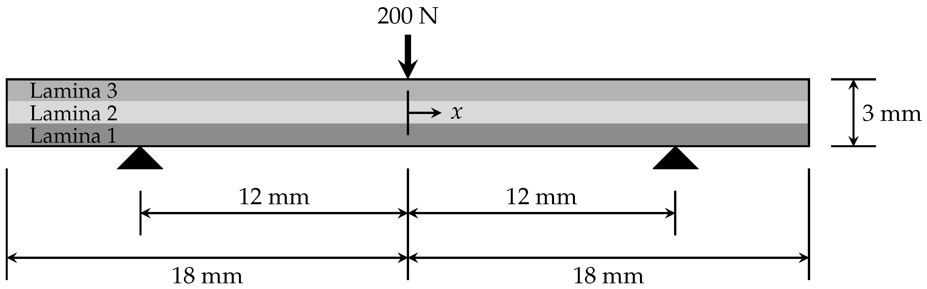
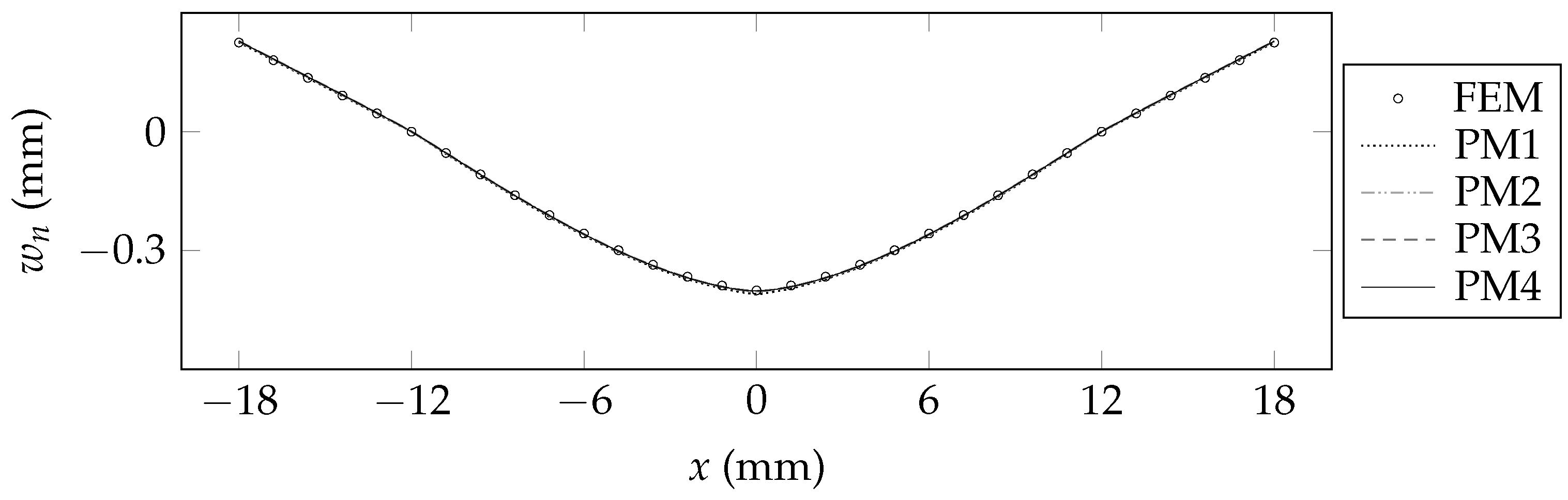
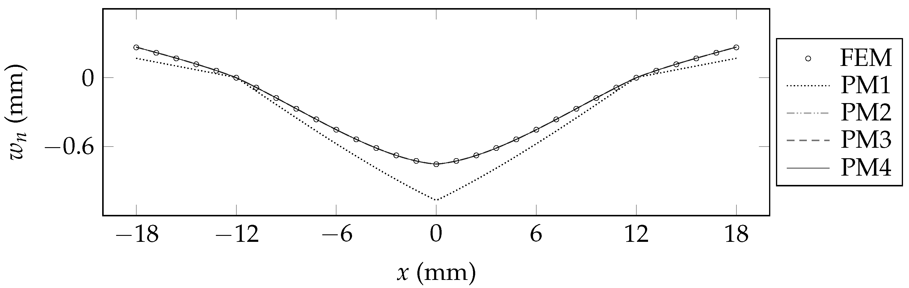
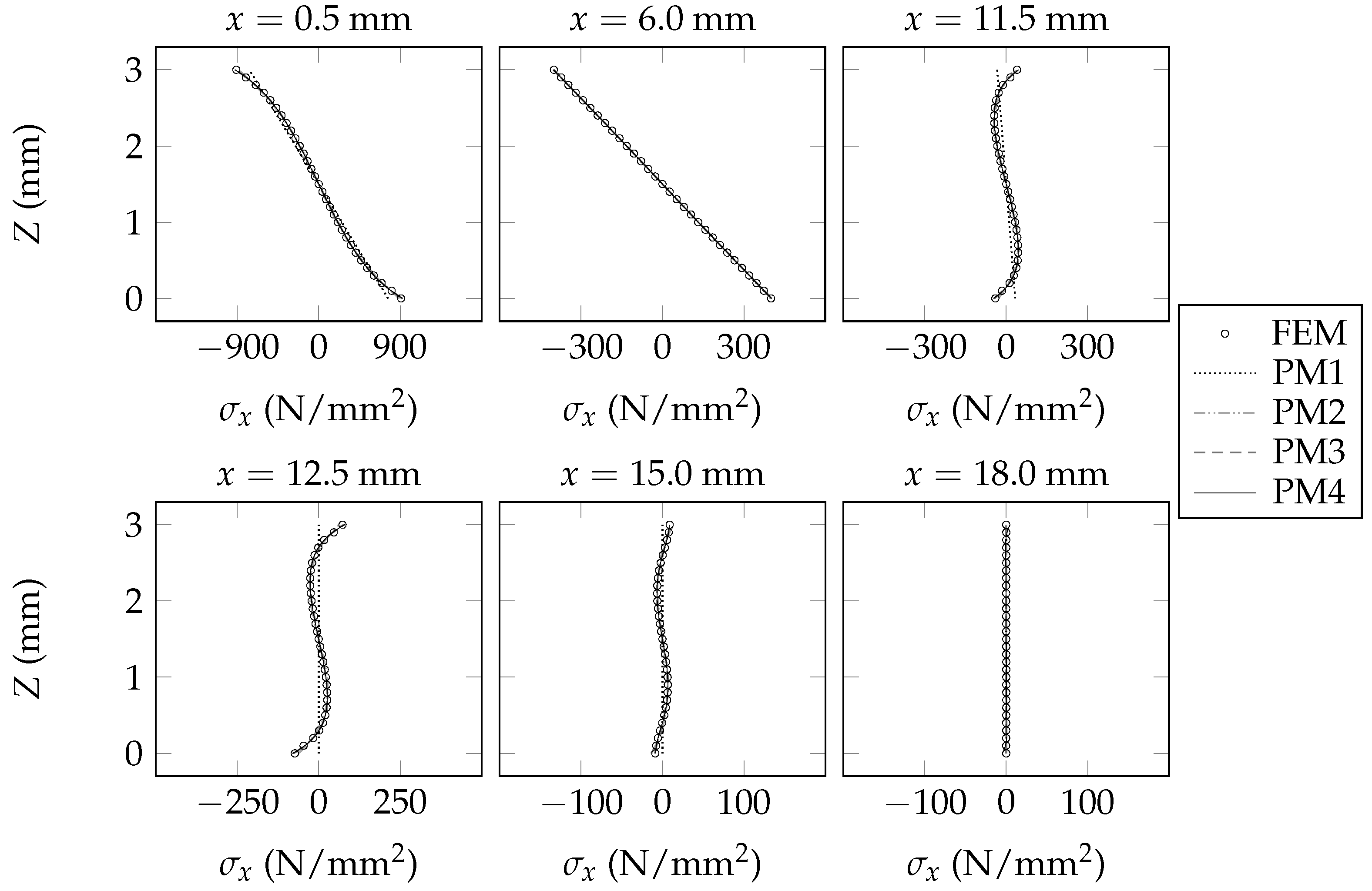
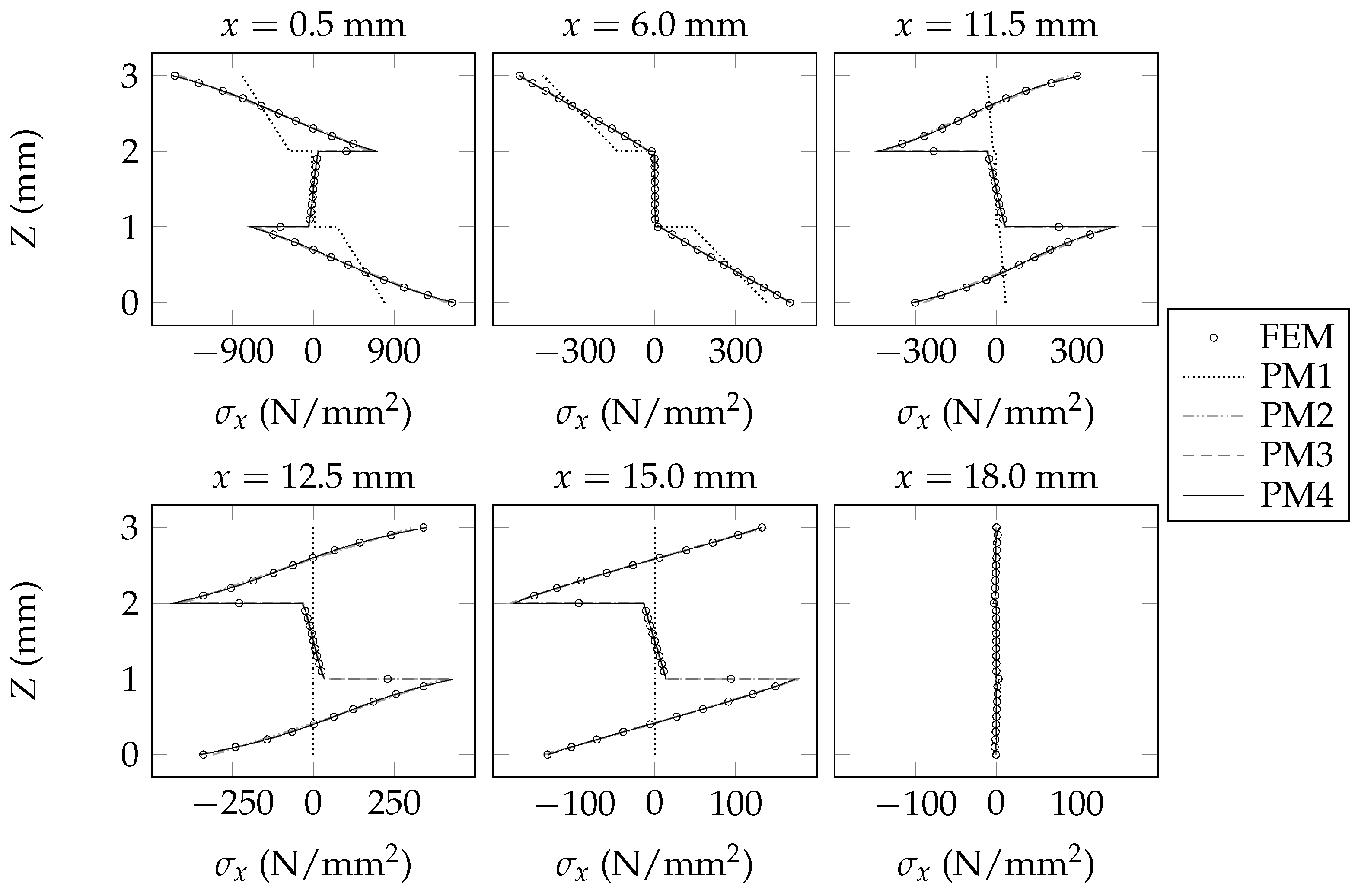
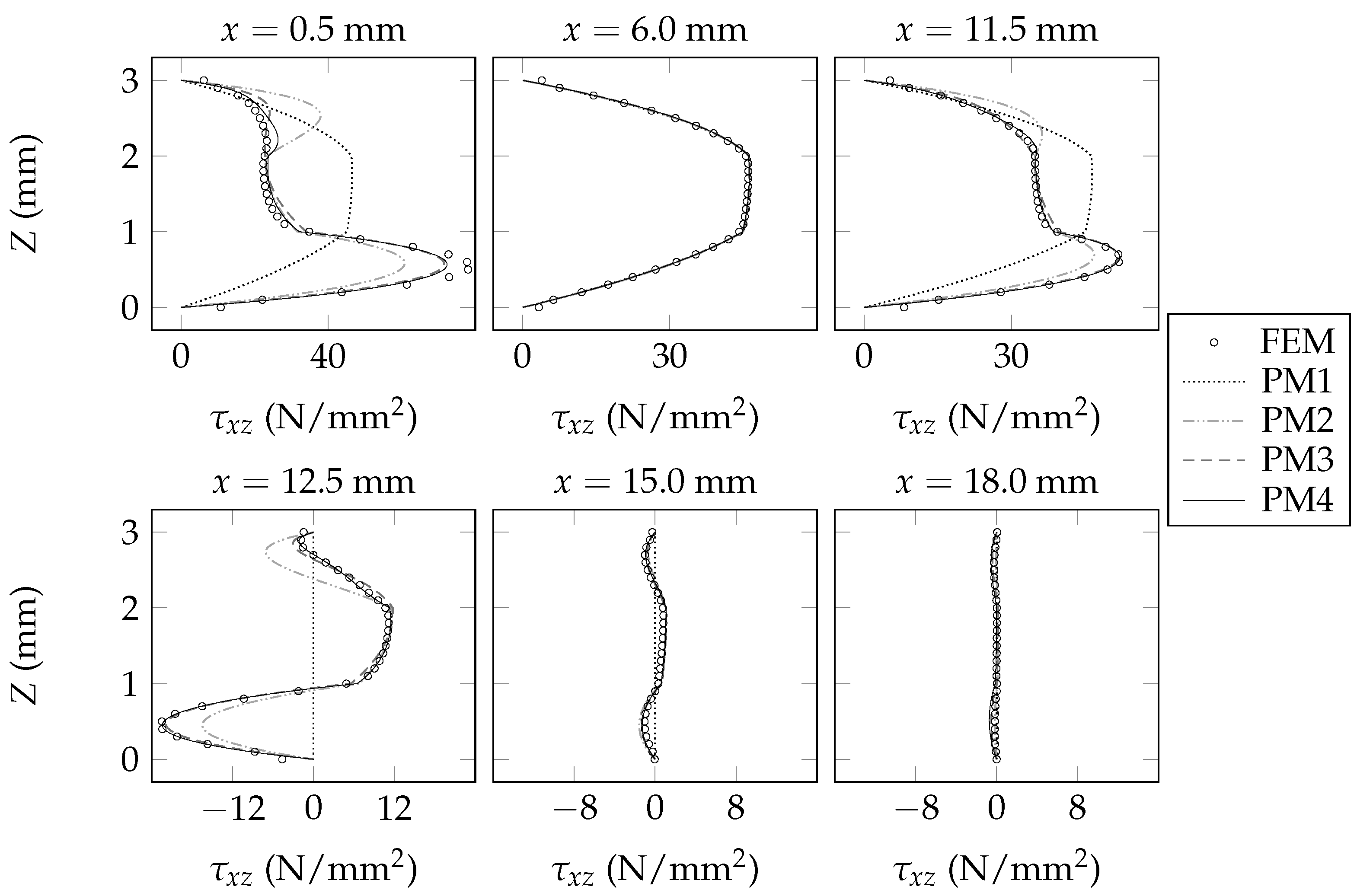
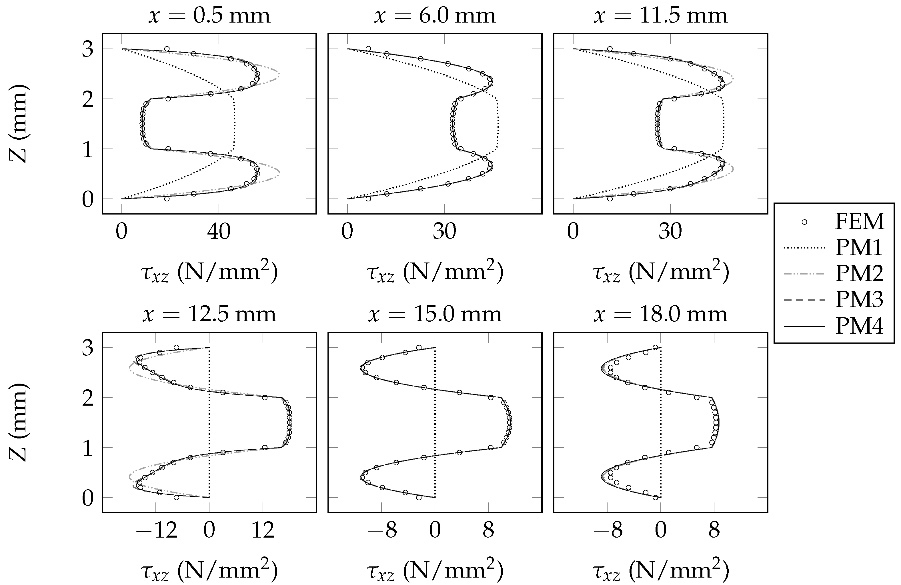
6. Validation of the Present Beam Model

A series of analyses were carried out in order to validate the present beam model. The present validation study was carried out in the context of three example beams that were previously presented in Ref. [5]. Some parts of the following descriptions are similar to descriptions that were provided in Ref. [5]; for greater clarity, the reader is directed to the Consent for Publication section of this article.
For the purpose of the present validation study, a single beam configuration was considered. This beam has a total length of 36 mm, and is symmetrically supported by two pin/roller supports that are positioned 24 mm apart. A single point load of 200 N is applied transversely (parallel to the z-axis) at the center of the beam. The aforementioned beam configuration and loading is illustrated in Figure 2.
Three example beams, each comprising a unique laminate, were considered for the present validation study. Each of the example beams exhibits the aforementioned beam configuration that is illustrated in Figure 2. Each of the example beams has a width of 1 mm, measured parallel to the y-axis. The three laminates that were considered are denoted by “Laminate A”, “Laminate B”, and “Laminate C”. Each laminate comprises three laminae. Each lamina has a thickness of 1 mm, measured parallel to the z-axis; therefore, each laminate has a total thickness of 3 mm, measured parallel to the z-axis. Laminate A comprises three identical laminae, which are each composed of a typical unidirectional carbon fiber reinforced polymer having its fibers initially oriented parallel to the x-axis. The upper lamina of Laminate B is composed of the same material as that which is present within Laminate A, the lower lamina of Laminate B is composed of a typical aluminium alloy, and the inner (core) lamina of Laminate B is composed of a typical unidirectional carbon fiber reinforced polymer having its fibers oriented parallel to the y-axis. The upper and lower laminae of Laminate C are each composed of the same material as that which is present within Laminate A, whereas the inner (core) lamina of Laminate C is composed of a material that is similar to a typical unidirectional carbon fiber reinforced polymer having its fibers oriented parallel to the y-axis, but with a shear modulus that is one tenth that of typical materials of this type. The aforementioned three laminates are summarized in Table 2.
“Beam A” denotes the beam that comprises Laminate A. “Beam B” denotes the beam that comprises Laminate B. “Beam C” denotes the beam that comprises Laminate C.
A MATLAB [25] implementation of the present beam model was used to predict the mechanical response of each of the three example beams, in accordance with the implementation procedure that is summarized in Section 5. Once the section constants and section functions were determined for each of the example beams, the governing equations were solved using the finite difference method with a grid spacing of 0.09 mm.
As a comparison with the present beam model, each of the three example beams was also analyzed using the finite element method. NX NASTRAN [26] was used for these finite element analyses. A detailed description of these finite element analyses is provided in Ref. [5].
In the interest of brevity, the following notation is employed herein: the present beam model with N = 1 is denoted by “PM1”, the present beam model with N = 2 is denoted by “PM2”, the present beam model with N = 3 is denoted by “PM3”, the present beam model with N = 4 is denoted by “PM4”, and the finite element model is denoted by “FEM”. It is worth reiterating that PM1 is equivalent to a Timoshenko beam theory analysis wherein the shear correction factor is calculated using the “directional shear energy” method that is discussed in Ref. [24].
The transverse deflections, w n , predicted by each model are shown in Figure 3, Figure 4 and Figure 5. For each of the FEM models, the transverse deflection at each position along the x-axis is taken as the mean of the z displacements of all of the nodes that are present at that x position. From examining Figure 3 and Figure 4, it is evident that each of PM1, PM2, PM3, and PM4 exhibits strong agreement with FEM for Beam A and Beam B; this can be attributed to the relative dominance of the first term of the governing differential equations for each of these beam configurations. Beam C exhibits non-trivial contributions from the higher-order terms of the governing differential equations; Figure 5 shows that PM1 over-predicts the transverse deflections of this beam, whereas PM2, PM3, and PM4 each exhibit strong agreement with FEM. Additionally, outside of the loaded span (for x < 12 mm and x > 12 mm), PM1 under-predicts the transverse deflections of Beam C, whereas PM2, PM3, and PM4 each closely follow the prediction of FEM.
The sectional fields of σ x predicted by each model are shown in Figure 6, Figure 7 and Figure 8. The sectional fields of τ x z predicted by each model are shown in Figure 9, Figure 10 and Figure 11. The sectional fields of σ x and τ x z are each plotted adjacent to the plane of symmetry ( x = 0.5 mm), midway between the plane of symmetry and the support ( x = 6 mm), adjacent to the support ( x = 11.5 mm and x = 12.5 mm), midway between the support and the free end of the beam ( x = 15 mm), and at the free end of the beam ( x = 18 mm). By inspecting Figure 6, Figure 7, Figure 8, Figure 9, Figure 10 and Figure 11, it is evident that the present beam model consistently offers successive improvements in analytical fidelity for each incremental increase in the value of N ; this trend is made particularly obvious upon careful inspection of the sectional fields of τ x z that are shown at x = 0.5 mm, x = 11.5 mm, and x = 12.5 mm. In the context of the presently assumed example beams, it is evident that the present beam model offers diminishing levels of improvement in analytical fidelity for each incremental increase in the value of N . For example, in the context of the presently assumed example beams, the improvement in analytical fidelity that is afforded by increasing the value of N from one to two appears to be greater than the improvement in analytical fidelity that is afforded by increasing the value of N from two to three.
In the context of the presently assumed example beams, the present validation study offers compelling evidence of the validity of the present beam model, and strongly supports the application of the present beam model for its intended purposes.

7. Concluding Remarks

In this study, a new unidimensional beam model was presented. The present beam model employs a recursive derivation procedure that enables the user to set the order of the governing differential equations as an input parameter, without the need for ad hoc assumptions or methodologies. The present article employed a novel system of kinematic variables, section constants, and section functions that facilitate the development of higher-order beam models that retain a clear philosophical link to classical beam models such as Euler–Bernoulli beam theory and Timoshenko beam theory. The present beam model is a type of equivalent single layer beam model, wherein section constants are used to model the global stiffness and compliance characteristics of the beam, and section functions are used to recover sectional fields of displacements, strains, and stresses. The present beam model is well suited for analyses of laminated beams that comprise any number of laminae. The present beam model was solved for several example beams, and the results were compared to the results of finite element analyses. It was shown that the present beam model is able to accurately predict the deformed shapes and stress fields of each of the example beams. From these example analyses, it is evident that the present beam model consistently offers successive improvements in analytical fidelity for each incremental increase in the number of terms that is included in the governing differential equations. However, it is also evident that the present beam model offers diminishing levels of improvement in analytical fidelity for each incremental increase in the number of terms that is included in the governing differential equations. The present article also revealed an interesting peculiarity of the elastic potential energy that pertains to any unidimensional beam model that is governed by differential equations that are of finite order.

8. Consent for Publication

Figure 2, Table 2, and the second and third paragraphs of Section 6 were originally presented in Ref. [5], and they have been reproduced and revised for inclusion in the present article, with permission, in accordance with the STM Permissions Guidelines (2022) [27]. Rights in Figure 2, Table 2, and the second and third paragraphs of Section 6 are owned by a third party, and permission for any further reuse of the aforementioned content must be obtained from the relevant holder of the exclusive rights.

Funding

This research received no external funding.

Data Availability Statement

The source code for the MATLAB [25] implementation of the present beam model is available from the corresponding author upon reasonable request. The NX NASTRAN [26] input and output files corresponding to the finite element analyses that are discussed herein are provided in an online archive [28].

Acknowledgments

The author wishes to acknowledge and thank Bruce Minaker and Stefan Kloppenborg for their participation in technical discussions related to the development of the present beam model.

Conflicts of Interest

The author declares no conflict of interest.

Appendix A. Supplementary Definitions

The term “mechanical centroid” denotes a specific point on each section of the beam; the mechanical centroid is positioned such that the following criterion is satisfied: if the beam is subjected to a uniform bending moment in the absence of any other applied loads, then each section of the beam will not develop any longitudinal normal strains at the position of its mechanical centroid. Therefore, at each section of the beam, the mechanical centroid represents the position of the intersection of the local y-y axis and the local z-z axis.
At each section of the beam, the mechanical centroid is contained in the longitudinal axis of the beam. In other words, the longitudinal axis of the beam intersects each section at the position of the mechanical centroid.
A longitudinal displacement is a displacement that occurs parallel to the x-axis. A longitudinal normal strain is a normal strain that is developed parallel to the x-axis. A longitudinal normal stress is a normal stress that acts parallel to the x-axis.
A transverse loading is a loading that acts perpendicular to the x-axis. A transverse shear force is a shear force that acts perpendicular to the x-axis.
The term “longitudinal elastic modulus” denotes the Young’s modulus of elasticity measured parallel to the x-axis.
The term “shear strain” herein denotes engineering shear strain.
The term “field” denotes a set of data that describes the value of a quantitative variable at each point that is contained in a particular geometric space. For example, a displacement field describes the displacement of each point that is contained in a particular geometric space.
The term “sectional field” denotes a set of data that describes the value of a quantitative variable at each point that is contained in a particular section of the beam. In other words, a sectional field is a field that pertains to the space that is embodied by a section of the beam. For example, a sectional field of τ x z describes the value of τ x z that is developed at each point that is contained in a particular section of the beam.
The term “initial orientation” herein denotes an orientation that is measured when the beam does not exhibit any deformation. For example, the initial orientation of each nominal sectional plane is defined such that the aforementioned nominal sectional plane is perpendicular to the x-axis.
The term “left curly bracket” denotes the symbol {. The term “right curly bracket” denotes the symbol }. The term “between curly brackets” is used in reference to notation that is shown between a left curly bracket and a right curly bracket, provided that the left curly bracket is positioned to the left of the aforementioned notation, and provided that the right curly bracket is positioned to the right of the aforementioned notation.

References

  1. Timoshenko, S. On the correction for shear of the differential equation for transverse vibrations of prismatic bars. Philos. Mag. 1921, 41, 744–746. [Google Scholar] [CrossRef] [Green Version]
  2. Timoshenko, S. On the transverse vibrations of bars of uniform cross-section. Philos. Mag. 1922, 43, 125–131. [Google Scholar] [CrossRef] [Green Version]
  3. Shi, G.; Voyiadjis, G. A Sixth-Order Theory of Shear Deformable Beams with Variational Consistent Boundary Conditions. J. Appl. Mech. 2011, 78, 021019. [Google Scholar] [CrossRef]
  4. Sapountzakis, E.; Argyridi, A. Literature Overview of Higher Order Beam Theories taking into account In-Plane and Out-of-Plane Deformation. J. Adv. Civ. Eng. Constr. Mater. 2018, 1, 1–15. [Google Scholar]
  5. Honickman, H.; Kloppenborg, S. A simple higher-order beam model that is represented by two kinematic variables and three section constants. Math. Mech. Solids 2021, 26, 1455–1482. [Google Scholar] [CrossRef]
  6. Reddy, J. A Simple Higher-Order Theory for Laminated Composite Plates. J. Appl. Mech. 1984, 51, 745–752. [Google Scholar] [CrossRef]
  7. Cook, G. A Higher-Order Bending Theory for Laminated Composite and Sandwich Beams; Contractor Report NASA/CR-201674; National Aeronautics and Space Administration, Langley Research Center: Hampton, VI, USA, 1997. [Google Scholar]
  8. Abadikhah, H. Higher Order Beam Equations. Master’s Thesis, Chalmers University of Technology, Göteborg, Sweden, 2011. [Google Scholar]
  9. Tessler, A.; Di Sciuva, M.; Gherlone, M. Refined Zigzag Theory for Homogeneous, Laminated Composite, and Sandwich Plates: A Homogeneous Limit Methodology for Zigzag Function Selection; Technical Publication NASA/TP-2010-216214; National Aeronautics and Space Administration, Langley Research Center: Hampton, VI, USA, 2010. [Google Scholar]
  10. Tessler, A.; Di Sciuva, M.; Gherlone, M. Refinement of Timoshenko Beam Theory for Composite and Sandwich Beams Using Zigzag Kinematics; Technical Publication NASA/TP-2007-215086; National Aeronautics and Space Administration, Langley Research Center: Hampton, VI, USA, 2007. [Google Scholar]
  11. Schulze, S.; Pander, M.; Naumenko, K.; Altenbach, H. Analysis of laminated glass beams for photovoltaic applications. Int. J. Solids Struct. 2012, 49, 2027–2036. [Google Scholar] [CrossRef]
  12. Loredo, A.; Castel, A. Two multilayered plate models with transverse shear warping functions issued from three dimensional elasticity equations. Compos. Struct. 2014, 117, 382–395. [Google Scholar] [CrossRef] [Green Version]
  13. Abrate, S.; Di Sciuva, M. Equivalent single layer theories for composite and sandwich structures: A review. Compos. Struct. 2017, 179, 482–494. [Google Scholar] [CrossRef]
  14. Arya, H.; Shimpi, R.; Naik, N. A zigzag model for laminated composite beams. Compos. Struct. 2002, 56, 21–24. [Google Scholar] [CrossRef]
  15. Tessler, A.; Di Sciuva, M.; Gherlone, M. A Refined Zigzag Beam Theory for Composite and Sandwich Beams. J. Compos. Mater. 2009, 43, 1051–1081. [Google Scholar] [CrossRef]
  16. Li, T. A (3,2) high order zigzag beam element: A unified zigzag function family. Compos. Struct. 2019, 208, 847–864. [Google Scholar] [CrossRef]
  17. Carrera, E.; Giunta, G. Refined beam theories based on a unified formulation. Int. J. Appl. Mech. 2010, 2, 117–143. [Google Scholar] [CrossRef]
  18. Carrera, E.; Giunta, G.; Petrolo, M. Chapter 4, A Modern and Compact Way to Formulate Classical and Advanced Beam Theories. In Developments and Applications in Computational Structures Technology; Saxe-Coburg Publications: Stirlingshire, UK, 2010; pp. 75–112. [Google Scholar] [CrossRef]
  19. Carrera, E.; Petrolo, M. Refined beam elements with only displacement variables and plate/shell capabilities. Meccanica 2012, 47, 537–556. [Google Scholar] [CrossRef]
  20. Carrera, E.; Cinefra, M.; Zappino, E.; Petrolo, M. Finite Element Analysis of Structures through Unified Formulation; John Wiley & Sons Ltd.: Hoboken, NJ, USA, 2014. [Google Scholar] [CrossRef]
  21. Minera, S.; Patni, M.; Carrera, E.; Petrolo, M.; Weaver, P.; Pirrera, A. Three-dimensional stress analysis for beam-like structures using Serendipity Lagrange shape functions. Int. J. Solids Struct. 2018, 141–142, 279–296. [Google Scholar] [CrossRef]
  22. Carrera, E.; Petrolo, M. Refined one-dimensional formulations for laminated structure analysis. AIAA J. 2012, 50, 176–189. [Google Scholar] [CrossRef]
  23. Arruda, M.; Castro, L.; Ferreira, A.; Garrido, M.; Gonilha, J.; Correia, J. Analysis of composite layered beams using Carrera unified formulation with Legendre approximation. Compos. Part B Eng. 2018, 137, 39–50. [Google Scholar] [CrossRef]
  24. Dong, S.; Alpdogan, C.; Taciroglu, E. Much ado about shear correction factors in Timoshenko beam theory. Int. J. Solids Struct. 2010, 47, 1651–1665. [Google Scholar] [CrossRef]
  25. MATLAB, Version 9.9.0.1467703 (R2020b); The MathWorks Inc.: Natick, MA, USA, 2020.
  26. NX NASTRAN, Version 12.0.1; Siemens Product Lifecycle Management Software Inc.: Plano, TX, USA, 2018.
  27. STM Permissions Guidelines; International Association of Scientific, Technical and Medical Publishers (STM), 2022. Available online: https://www.stm-assoc.org/intellectual-property/permissions/permissions-guidelines/ (accessed on 4 April 2022).
  28. Honickman, H.; Kloppenborg, S. Supplemental Material for the Article Entitled “A Simple Higher-Order Beam Model That Is Represented by Two Kinematic Variables and Three Section Constants”, Version 1.1.0. 2020. Available online: https://zenodo.org/record/4274199#.Y8-WGHbMKUk/ (accessed on 1 February 2022).
Figure 1. Deformed shape of a transversely loaded beam, illustrating some of the geometric dimensions and kinematic variables that are relevant to the present beam model.
Applmech 04 00008 g001
Figure 2. Loading configuration of the example beams used to validate the present beam model [5]. The reader is directed to the Consent for Publication section.
Applmech 04 00008 g002
Figure 3. Transverse deflections of Beam A.
Applmech 04 00008 g003
Figure 4. Transverse deflections of Beam B.
Applmech 04 00008 g004
Figure 5. Transverse deflections of Beam C.
Applmech 04 00008 g005
Figure 6. Sectional fields of longitudinal normal stresses within Beam A.
Applmech 04 00008 g006
Figure 7. Sectional fields of longitudinal normal stresses within Beam B.
Applmech 04 00008 g007
Figure 8. Sectional fields of longitudinal normal stresses within Beam C.
Applmech 04 00008 g008
Figure 9. Sectional fields of x-z shear stresses within Beam A.
Applmech 04 00008 g009
Figure 10. Sectional fields of x-z shear stresses within Beam B.
Applmech 04 00008 g010
Figure 11. Sectional fields of x-z shear stresses within Beam C.
Applmech 04 00008 g011
Table 1. Present beam model’s treatment of some common boundary conditions.
Physical ConstraintBoundary Conditions at Position of Constraint
Roller (no transverse deflection) w n = 0
Guided (no rotation) d w n d x = 0
Fixed (clamped) w n = 0 , ϕ w = 0 , and  d ( 2 j 2 ) ϕ w d x ( 2 j 2 ) = 0
Free End d ( 2 j 1 ) ϕ w d x ( 2 j 1 ) = 0
where j is an integer value that satisfies 0 < j N .
Table 2. Laminates employed in the example beams used to validate the present beam model [5]. The reader is directed to the Consent for Publication section.
Laminate ALaminate BLaminate C
Lamina 3Carbon 0 Carbon 0 Carbon 0
E = 119,000 N / mm 2 E = 119,000 N / mm 2 E = 119,000 N / mm 2
G = 4230   N / mm 2 G = 4230   N / mm 2 G = 4230   N / mm 2
Thickness = 1 mm Thickness = 1 mm Thickness = 1 mm
Lamina 2Carbon 0 Carbon 90 Modified Carbon 90
E = 119,000 N / mm 2 E = 9270   N / mm 2 E = 9270   N / mm 2
G = 4230   N / mm 2 G = 3228   N / mm 2 G = 323   N / mm 2
Thickness = 1 mm Thickness = 1 mm Thickness = 1 mm
Lamina 1Carbon 0 AluminiumCarbon 0
E = 119,000 N / mm 2 E = 68,900 N / mm 2 E = 119,000 N / mm 2
G = 4230   N / mm 2 G = 26,200 N / mm 2 G = 4230   N / mm 2
Thickness = 1 mm Thickness = 1 mm Thickness = 1 mm
Disclaimer/Publisher’s Note: The statements, opinions and data contained in all publications are solely those of the individual author(s) and contributor(s) and not of MDPI and/or the editor(s). MDPI and/or the editor(s) disclaim responsibility for any injury to people or property resulting from any ideas, methods, instructions or products referred to in the content.

