Anisortopic Modeling of Hydraulic Fractures Height Growth in the Anadarko Basin


Abstract
:1. Introduction
2. Problem Statement
3. Stress Estimation
4. Methodology
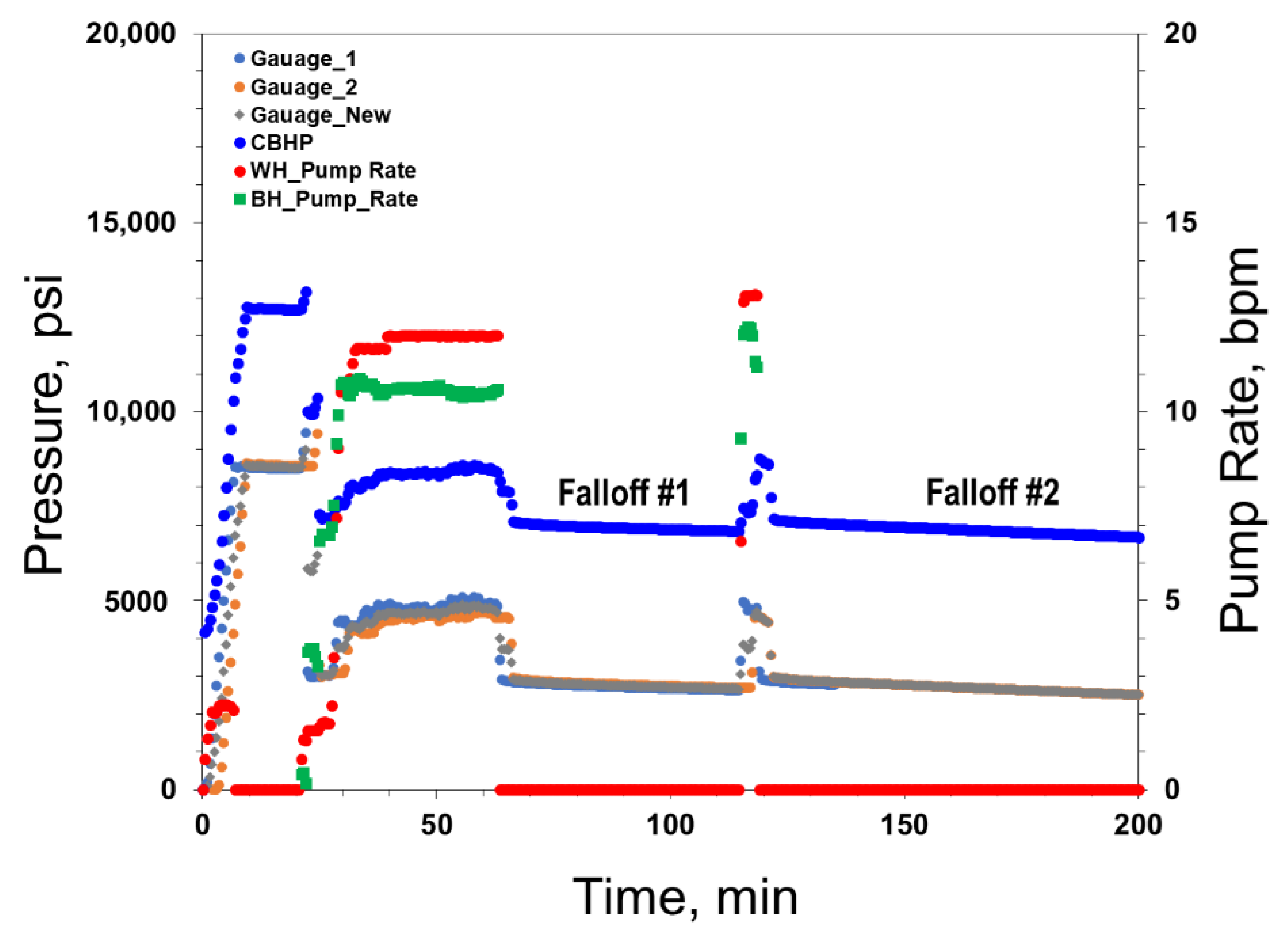
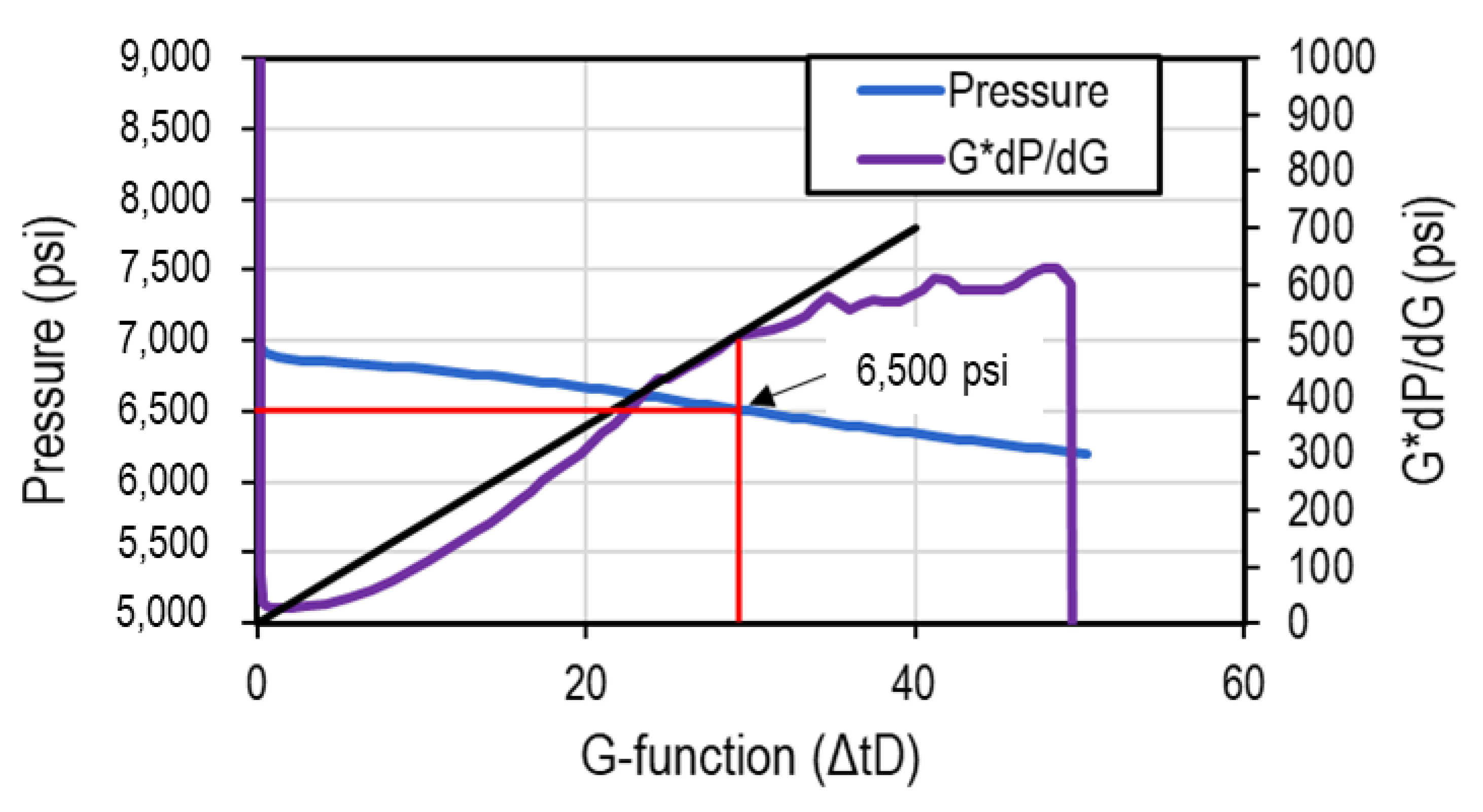
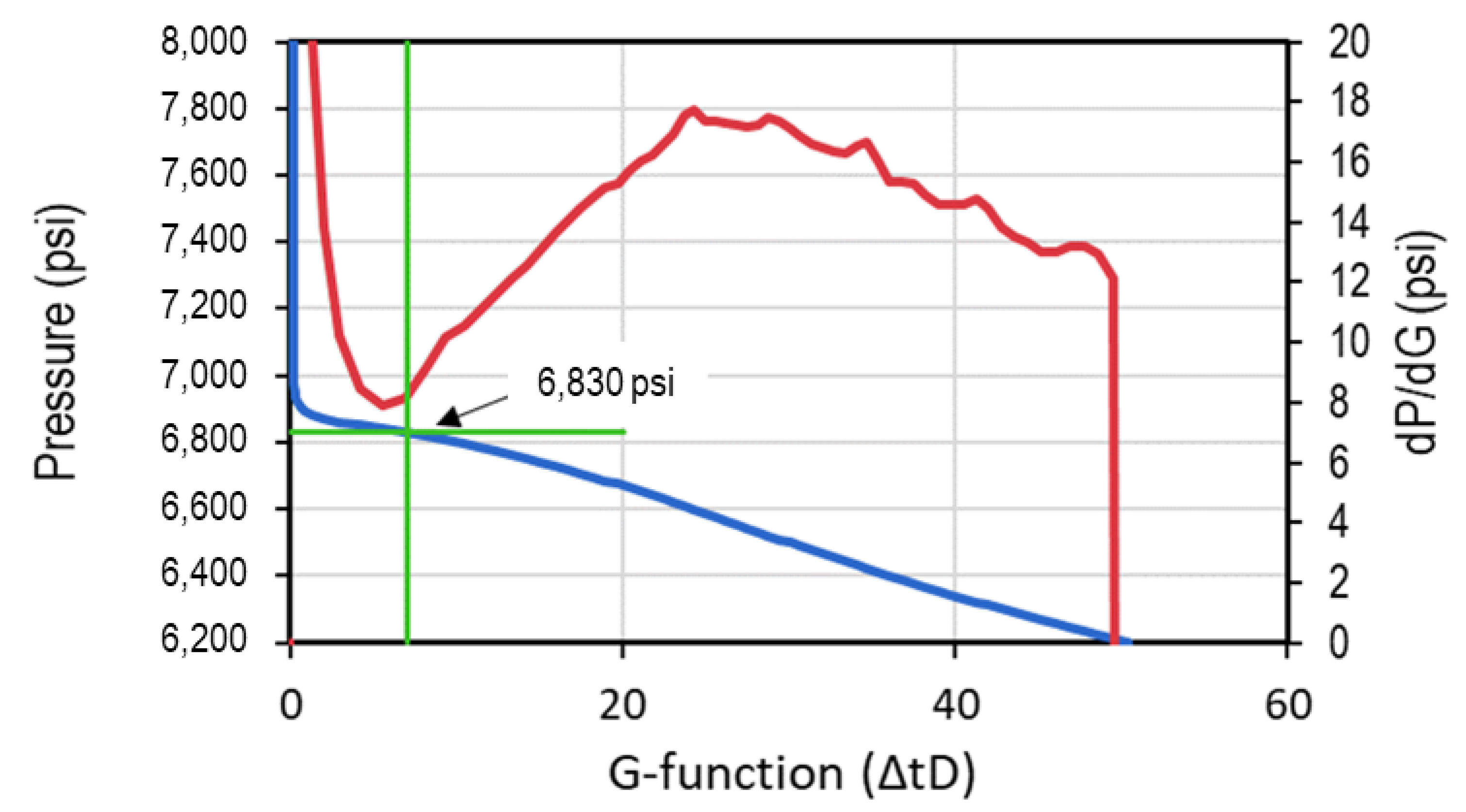
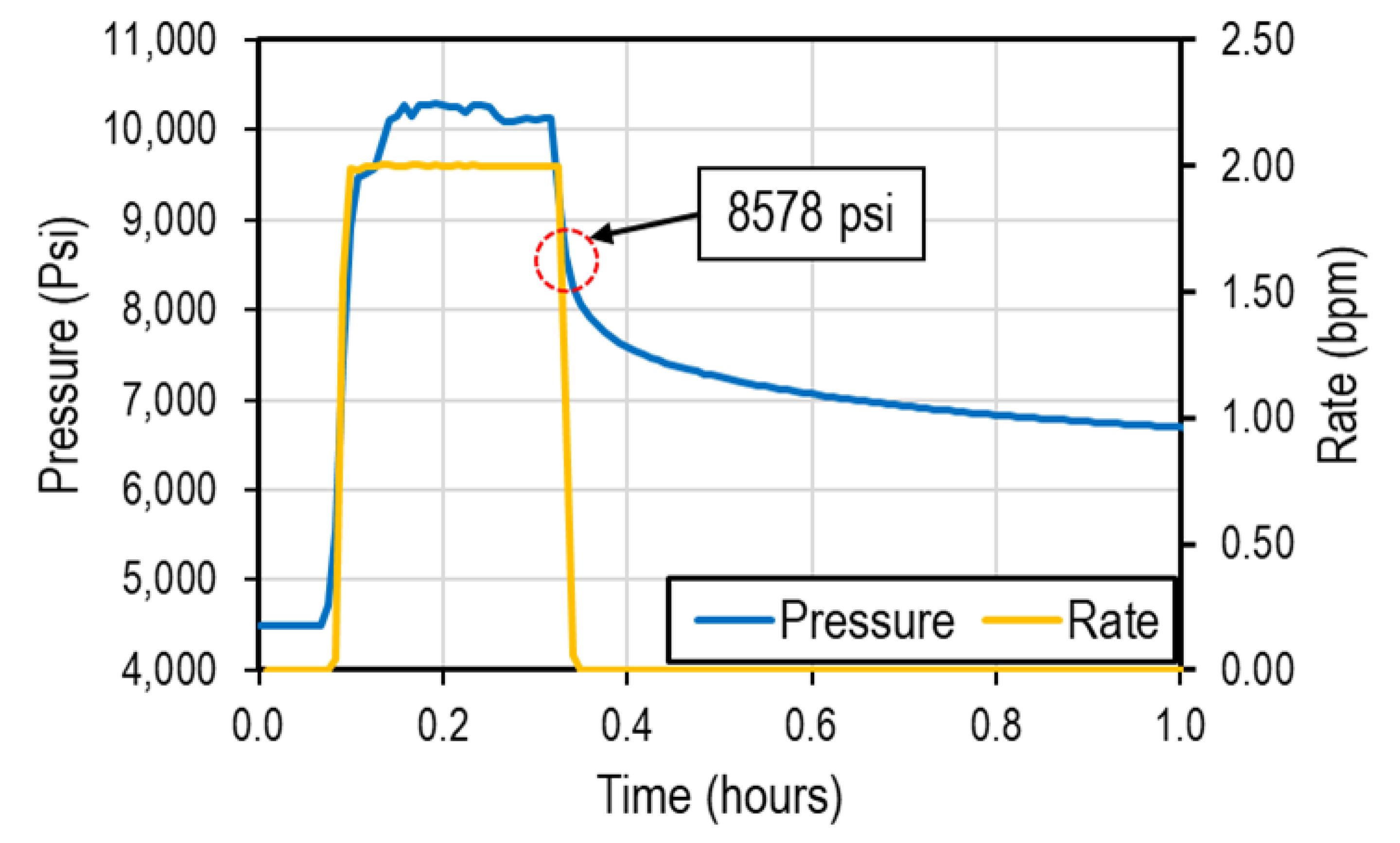
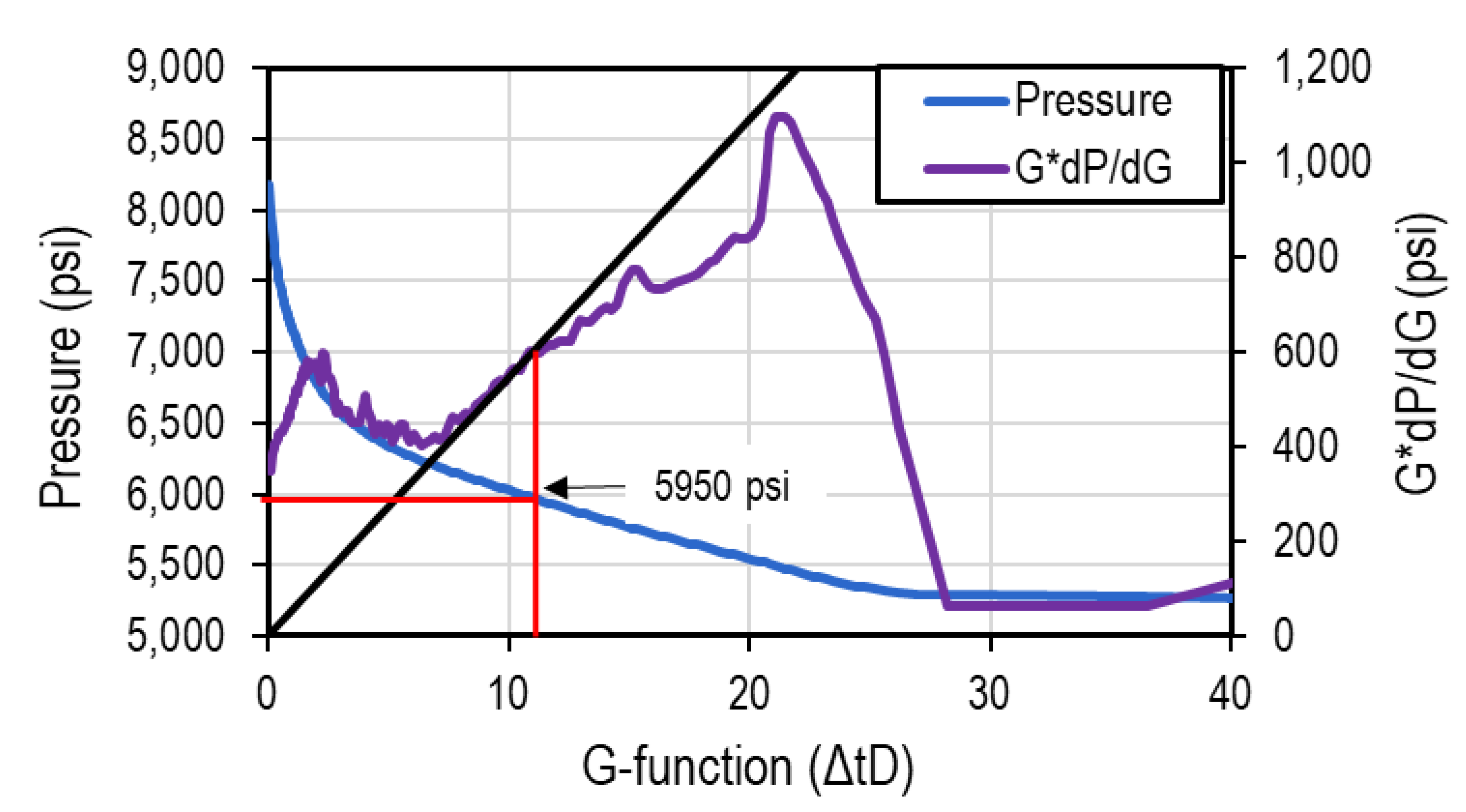
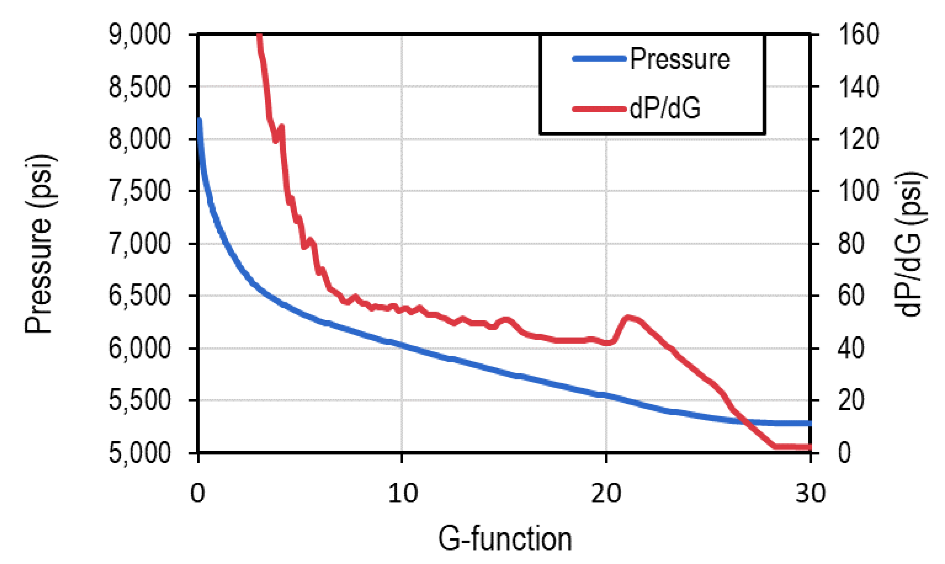
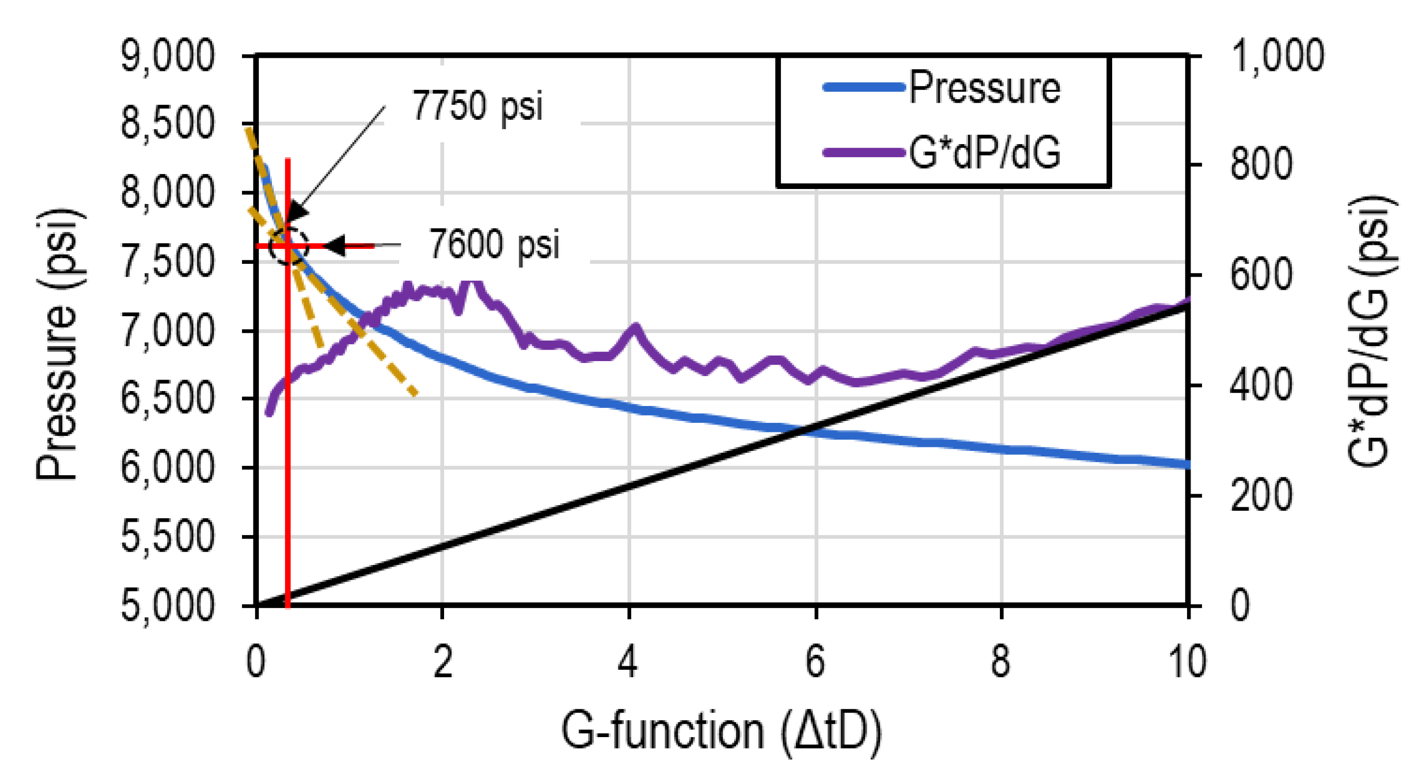
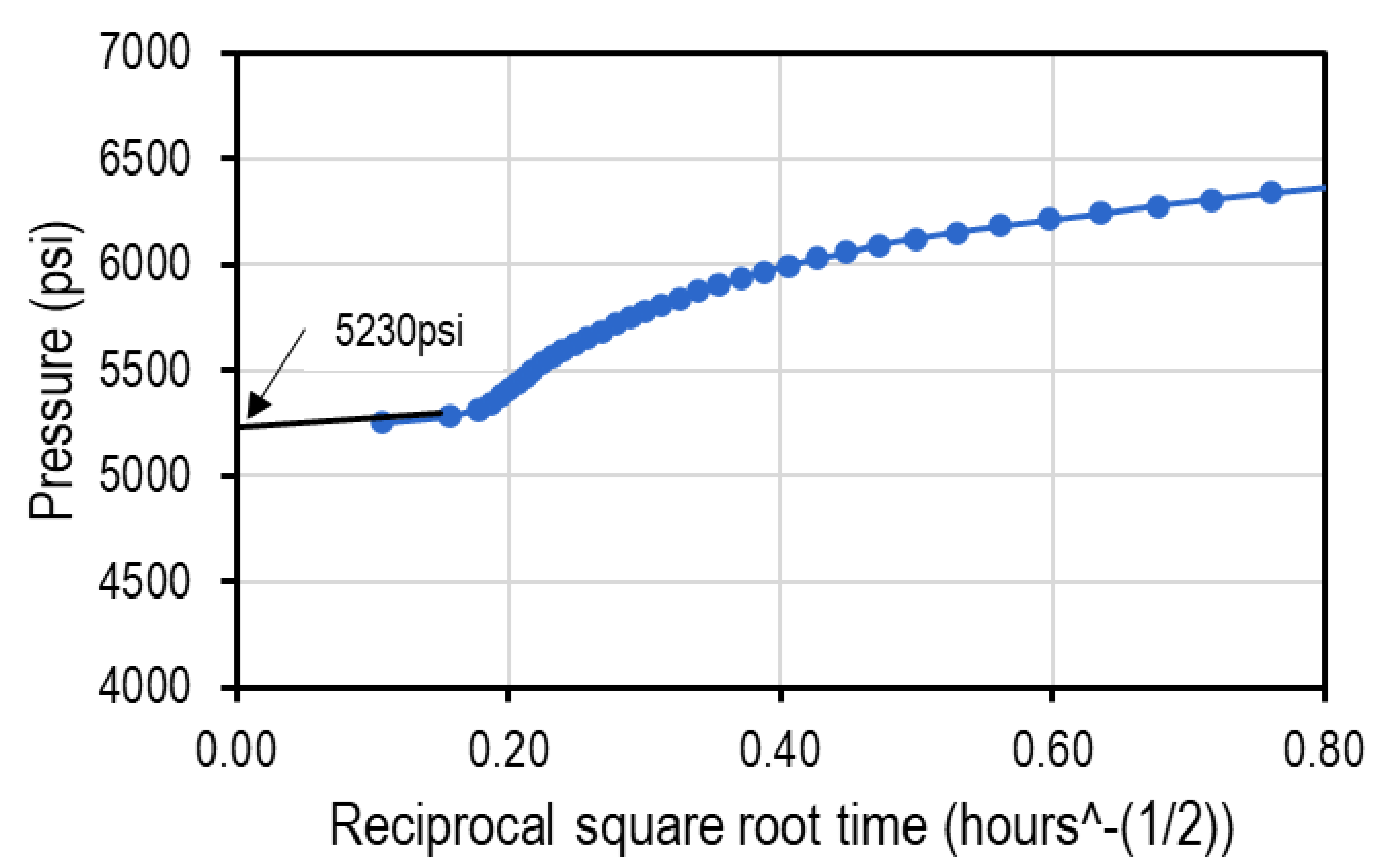
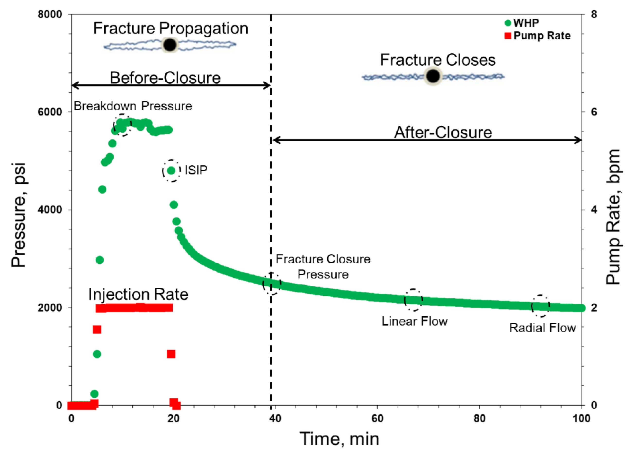
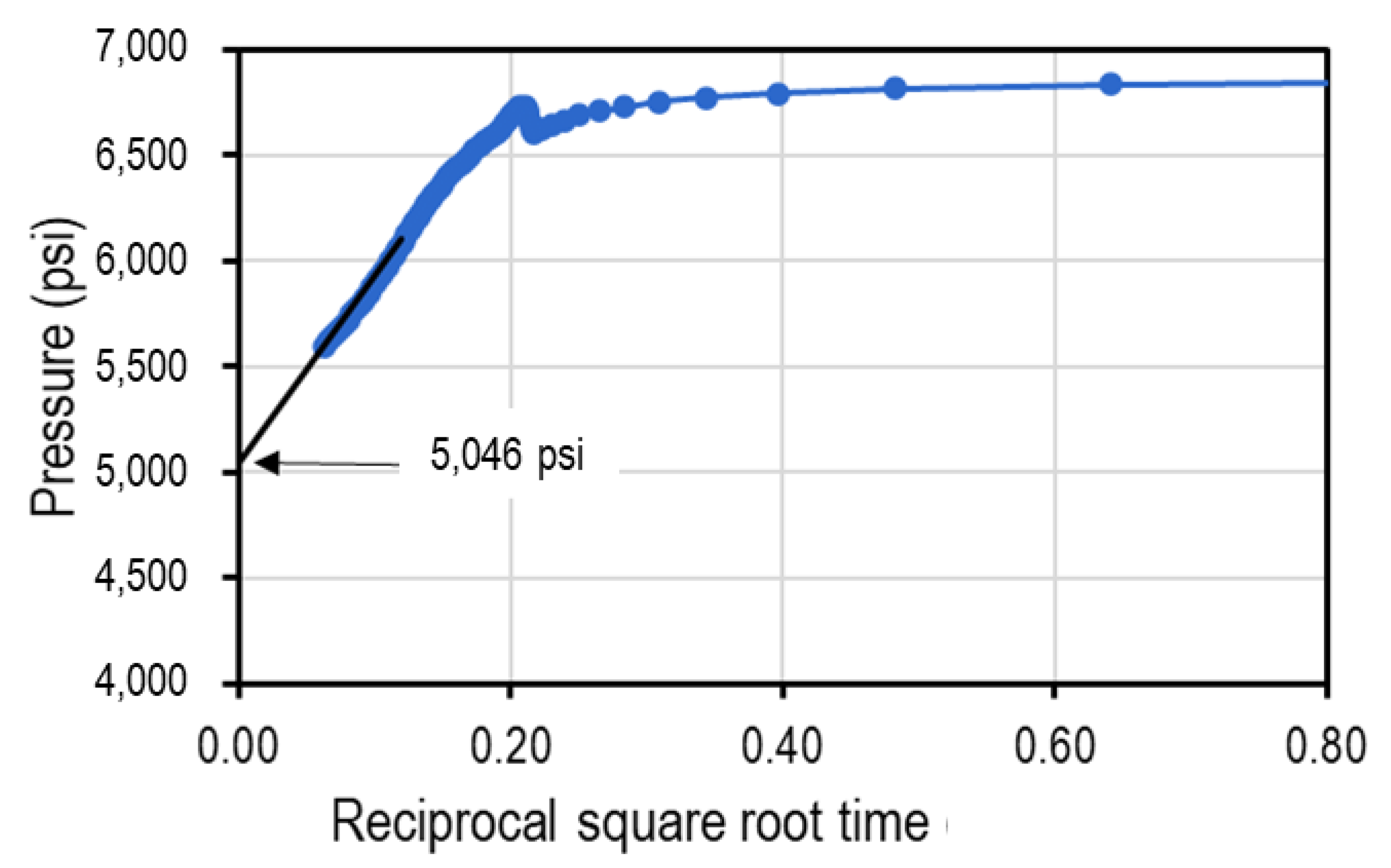
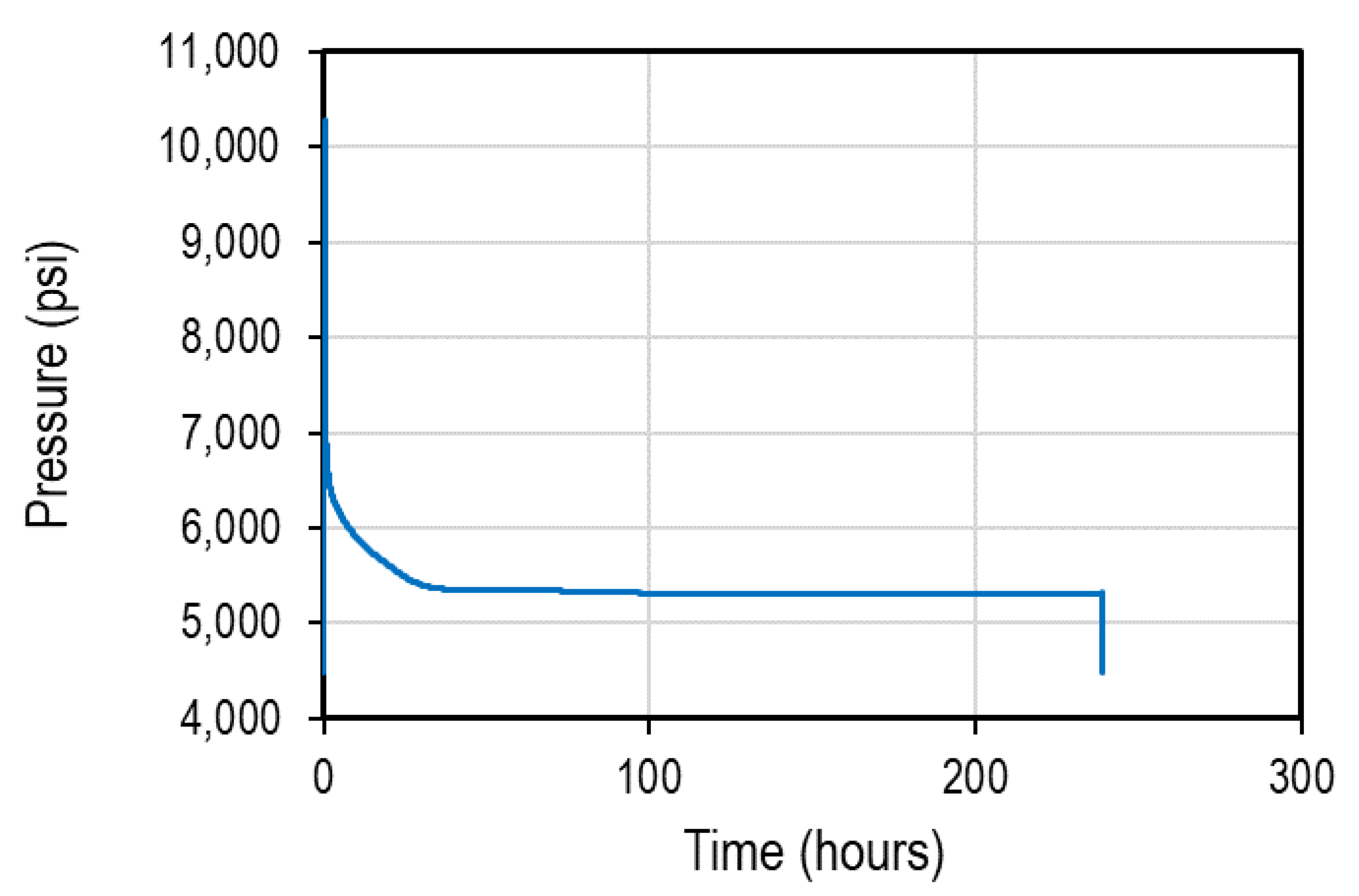
4.1. DFIT Analysis
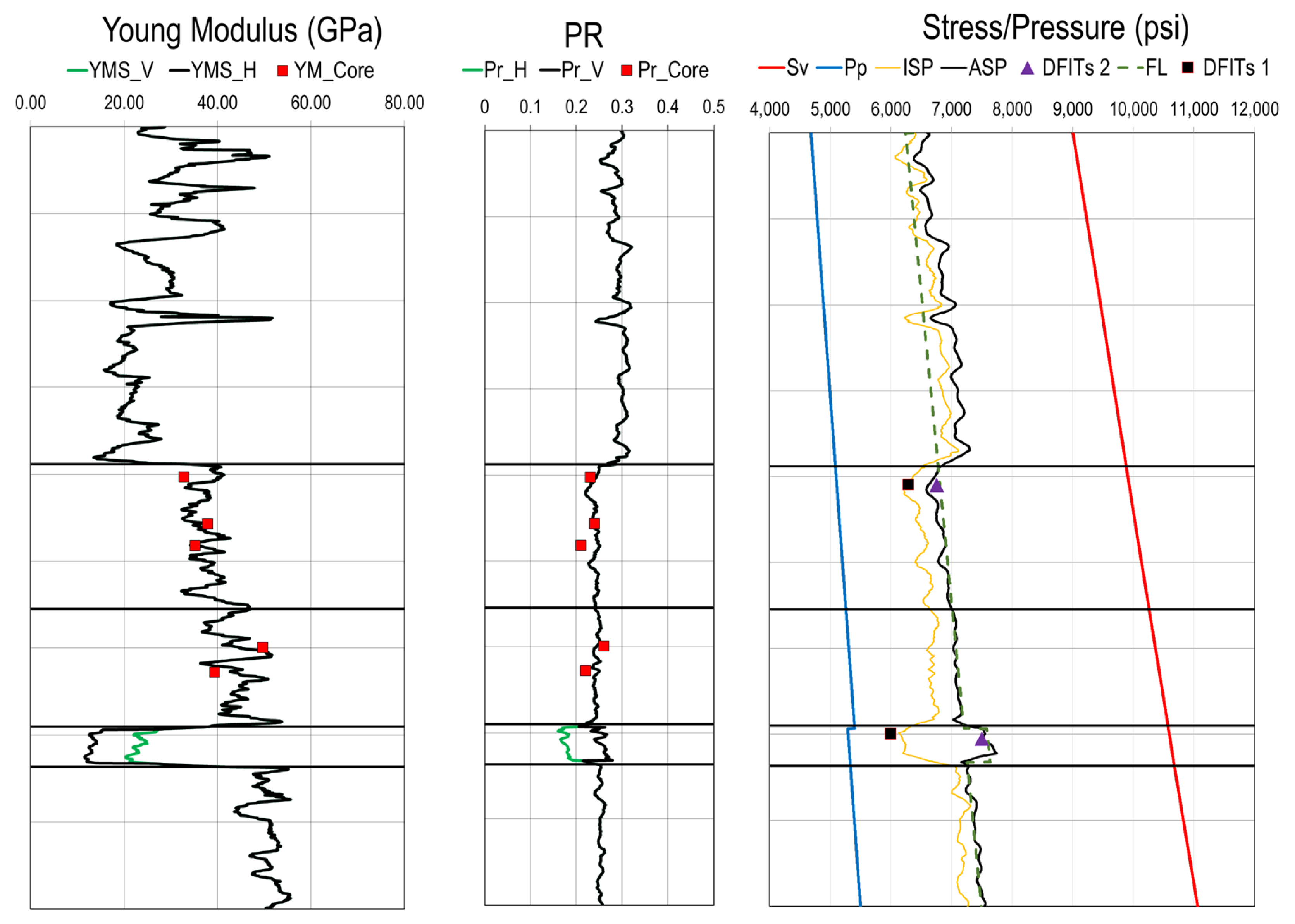
4.2. Stress Model
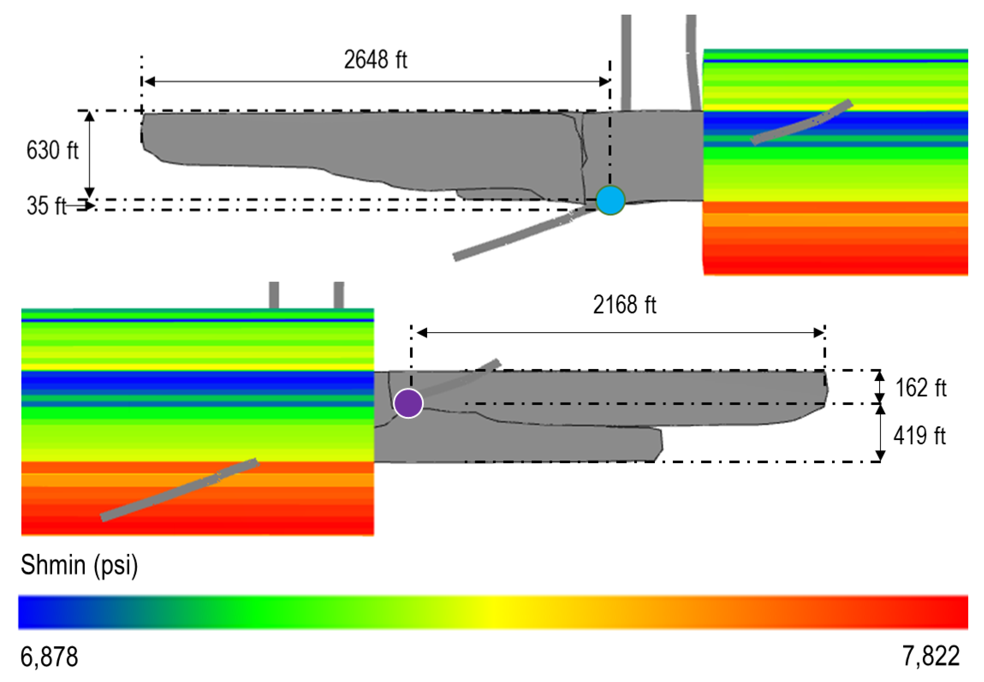
4.3. Numerical Modeling
- Fracture toughness of and relative fracture toughness of 0.5 .
- Pore pressure and stresses from the MEM.
- Leak-off calculated from fluid flow using permeability (see Appendix A).
- Crossed relative permeability curves.
- A fracture mesh size of 100 ft and a wellbore mesh size of 15 ft.
- A geomodel with 1530 ft height, 10,000 ft length, and 1100 ft wide.
- A total of 122,518 grids (25i, 100j, 49k).
5. Results and Discussion
6. Conclusions
- The method of DFIT analysis may lead to erroneous estimation of stress because of the geological complexity of the formation, so it is essential to QC that the DFIT results use values that are not very low compared with the ISIP, World Stress map, values from the literature, and the frictional limit theory.
- Several interpretation techniques for the DFIT need to be conducted to reduce the uncertainty of one method over the other.
- In heterogeneous formations with different clay and kerogen content, it is preferable to conduct several DFITs and account for kerogen and clay content to ensure reliable estimates.
- The anisotropic model can capture the higher stress values in formations with high clay content, while using the isotropic approach can lead to very low values.
Author Contributions
Funding
Data Availability Statement
Acknowledgments
Conflicts of Interest
Appendix A

| Sample | Permeability | Porosity | Saturation | |
|---|---|---|---|---|
| Depth | Millidarcies | % | % | |
| feet | Air | Ambient | Water | Oil |
| 9744.97 | 0.000135 | 1.9 | 76.7 | 18.1 |
| 9751.99 | 0.000027 | 1.5 | 57.5 | 26.7 |
| 9763.96 | 0.000136 | 2.1 | 68.1 | 12.5 |
| 9780.08 | 0.000445 | 4.4 | 62.9 | 26.4 |
| 9820.00 | 0.000159 | 4.0 | 51.5 | 31.9 |
| 9825.97 | 0.000118 | 2.3 | 49.2 | 35.0 |
| 9839.99 | 0.000075 | 2.2 | 81.7 | 15.6 |
| 9860.03 | 0.000109 | 3.9 | 48.7 | 28.1 |
| 9880.08 | 0.000119 | 4.2 | 62.8 | 28.0 |
| 9886.01 | 0.000010 | 1.9 | 66.6 | 21.5 |
| 9899.00 | 0.000139 | 1.4 | 77.3 | 15.2 |
| 9904.97 | 0.000132 | 2.4 | 32.2 | 36.4 |
| 9923.03 | 0.000056 | 2.3 | 55.3 | 26.0 |
| 9945.98 | 0.000399 | 3.5 | 71.1 | 23.0 |
| 9955.00 | 0.000193 | 5.2 | 15.0 | 34.3 |
| 9999.01 | 0.000116 | 2.2 | 49.8 | 31.7 |
| 10,007.01 | 0.000380 | 1.2 | 36.8 | 14.4 |
| 10,014.04 | 0.000067 | 2.1 | 50.6 | 29.8 |
| 10,022.03 | 0.000141 | 1.6 | 62.2 | 22.5 |
| 10,034.04 | 0.000179 | 3.6 | 79.5 | 17.5 |
| 10,060.01 | 0.000208 | 1.3 | 74.6 | 6.8 |
| 10,110.06 | 0.000082 | 1.3 | 62.8 | 11.3 |
| 10,122.01 | 0.000085 | 1.8 | 78.2 | 6.2 |
| 10,133.94 | 0.000099 | 0.4 | ||
| 10,150.96 | 0.000066 | 1.3 | ||
| 10,163.96 | 0.000003 | 0.6 | ||
| 10,247.99 | 0.000131 | 2.3 | 85.7 | 11.8 |
| 10,286.95 | 0.000004 | 0.8 | ||
References
- Abousleiman, Y.N.; Tran, M.H.; Hoang, S.; Bobko, C.P.; Ortega, A.; Ulm, F.-J. Geomechanics Field and Laboratory Characterization of the Woodford Shale: The Next Gas Play. In Proceedings of the SPE Annual Technical Conference and Exhibition, Anaheim, CA, USA, 11–14 November 2007; Volume 4, pp. 2127–2140. [Google Scholar] [CrossRef]
- Aoun, A.E.; Soto, R.; Rabiei, M.; Rasouli, V.; Khetib, Y.; Irofti, D. Neural Network based Mechanical Earth Modelling (MEM): A case study in Hassi Messaoud Field, Algeria. J. Pet. Sci. Eng. 2021, 210, 110038. [Google Scholar] [CrossRef]
- Barree, R.D.; Miskimins, J.L.; Gilbert, J.V. Diagnostic Fracture Injection Tests: Common Mistakes, Misfires and Mis-Diagnoses. In Proceedings of the Society of Petroleum Engineers—SPE Western North American and Rocky Mountain Joint Meeting, Denver, CO, USA, 15–18 April 2014. [Google Scholar]
- Belayouni, N.; Katz, D.; Grechka, V.; Christianson, P. Microseismic Event Location Using the Direct and Reflected Waves—A Woodford Case Study. In Proceedings of the 79th EAGE Conference and Exhibition, Paris, France, 12–15 June 2017; pp. 3981–3986. [Google Scholar] [CrossRef]
- Ben Naceur, K.; Touboul, E. Mechanisms Controlling Fracture-Height Growth in Layered Media. SPE Prod. Eng. 1990, 5, 142–150. [Google Scholar] [CrossRef]
- Laalam, A.; Berrehal, B.E.; Chemmakh, A.; Ouadi, H.; Merzoug, A.; Djezzar, S.; Boualam, A. A New Perspective for the Conception of Mechanical Earth Model Using Machine Learning in The Volve Field, Norwegian North Sea. In Proceedings of the 56th U.S. Rock Mechanics/Geomechanics Symposium, Santa Fe, NM, USA, 26–29 June 2022. [Google Scholar] [CrossRef]
- Boualam, A.; Djezzar, S.; Rasouli, V.; Rabiei, M. 3D Modeling and Natural Fractures Characterization. In Proceedings of the 53rd U.S. Rock Mechanics/Geomechanics Symposium, New York, NY, USA, 26–29 June 2019. [Google Scholar]
- Cipolla, C.; Litvak, M.; Prasad, R.S.; McClure, M. Case History of Drainage Mapping and Effective Fracture Length in the Bakken. In Proceedings of the SPE Hydraulic Fracturing Technology Conference and Exhibition, The Woodlands, TX, USA, 4–6 February 2020; pp. 1–43. [Google Scholar] [CrossRef]
- Dontsov, E. A Continuous Fracture Front Tracking Algorithm with Multi Layer Tip Elements (MuLTipEl) for a Plane Strain Hydraulic Fracture. arXiv 2021, arXiv:2104.11184. [Google Scholar] [CrossRef]
- Economides, M.; Nolte, K. Reservior Stimulation; Wiley: New York, NY, USA, 2000; p. 824. [Google Scholar]
- Ellafi, A.; Jabbari, H. Understanding the Mechanisms of Huff-n-Puff, CO2-EOR in Liquid-Rich Shale Plays: Bakken Case Study. In Proceedings of the SPE Canada Unconventional Resources Conference, Virtual, 28 September–2 October 2020. [Google Scholar] [CrossRef]
- Ellafi, A.; Jabbari, H. Unconventional Well Test Analysis for Assessing Individual Fracture Stages through Post-Treatment Pressure Falloffs: Case Study. Energies 2021, 14, 6747. [Google Scholar] [CrossRef]
- Ellafi, A.; Jabbari, H.; Tomomewo, O.S.; Mann, M.D.; Geri, M.B.; Tang, C. Future of Hydraulic Fracturing Application in Terms of Water Management and Environmental Issues: A Critical Review. In Proceedings of the SPE Canada Unconventional Resources Conference, Virtual, 28 September–2 October 2020. [Google Scholar] [CrossRef]
- Fisher, M.K.; Warpinski, N.R. Hydraulic-Fracture-Height Growth: Real Data. SPE Prod. Oper. 2012, 27, 8–19. [Google Scholar] [CrossRef]
- Fjær, E.; Holt, R.; Horsrud, P.; Raaen, A. Petroleum Related Rock Mechanics; SPE Reservoir Engineering (Society of Petroleum Engineers); Elsevier: Amsterdam, The Netherlands, 2008; Volume 9, ISBN 9780080557090. [Google Scholar]
- Frydman, M.; Pacheco, F.; Pastor, J.; Canesin, F.C.; Caniggia, J.; Davey, H. Comprehensive Determination of the Far-Field Earth Stresses for Rocks with Anisotropy in Tectonic Environment. In Proceedings of the SPE Argentina Exploration and Production of Unconventional Resources Symposium, Buenos Aires, Argentina, 1–3 June 2016; pp. 1–14. [Google Scholar] [CrossRef]
- Ganpule, S.; Srinivasan, K.; Izykowski, T.; Luneau, B.; Gomez, E. Impact of Geomechanics on Well Completion and Asset Development in the Bakken Formation. In Proceedings of the SPE Hydraulic Fracturing Technology Conference, The Woodlands, TX, USA, 4–6 February 2015. [Google Scholar] [CrossRef]
- Grieser, W.V. Oklahoma Woodford Shale: Completion Trends and Production Outcome from Three Basins. In Proceedings of the SPE Production and Operations Symposium, Oklahoma City, OK, USA, 27–29 March 2011; pp. 19–35. [Google Scholar] [CrossRef]
- Guglielmi, Y.M.; Burghardt, J.; Joseph, P.M.; Doe, T.; Fu, P.; Knox, H. Estimating Stress from Fracture Injection Tests: Comparing Pressure Transient Interpretations with In-Situ Strain Measurements. In Proceedings of the Stanford Geothermal Workshop, Stanford, CA, USA, 11–13 February 2022; pp. 1–19. [Google Scholar]
- Gupta, I.; Rai, C.; Devegowda, D.; Sondergeld, C.H. Fracture Hits in Unconventional Reservoirs: A Critical Review. SPE J. 2021, 26, 412–434. [Google Scholar] [CrossRef]
- Qu, H.; Liu, Y.; Zhou, C.; Ren, L.; Wei, Q.; Lv, Y.; Hou, J. The Characteristics of Hydraulic Fracture Growth in Woodford Shale, the Anadarko Basin. In Proceedings of the SPE/IATMI Asia Pacific Oil & Gas Conference and Exhibition, Jakarta, Indonesia, 17–19 October 2017. [Google Scholar] [CrossRef]
- Haustveit, K.; Elliott, B.; Roberts, J. Empirical Meets Analytical-Novel Case Study Quantifies Fracture Stress Shadowing and Net Pressure Using Bottom Hole Pressure and Optical Fiber. In Proceedings of the SPE Hydraulic Fracturing Technology Conference and Exhibition, The Woodlands, TX, USA, 31 January–2 February 2022. [Google Scholar] [CrossRef]
- Higgins, S.M.; Goodwin, S.A.; Donald, A.; Bratton, T.R.; Tracy, G.W. Anisotropic Stress Models Improve Completion Design in the Baxter Shale. In Proceedings of the SPE Annual Technical Conference and Exhibition, Denver, CO, USA, 21–24 September 2008; pp. 2076–2085. [Google Scholar] [CrossRef]
- Hryb, D.E.; Diaz, A.; Tomassini, F.G. High Resolution Geomechanical Model and its Impact on Hydraulic Fracture Height Growth. An Example from Vaca Muerta Formation, Argentina. In Proceedings of the 2020 Latin America Unconventional Resources Technology Conference, Buenos Aires, Argentina, 16–18 November 2020. [Google Scholar] [CrossRef]
- Jaeger, J.C.; Cook, N.G.W.; Robert, Z. Fundamentals of Rock Mechanics; Willey: New York, NY, USA, 2007. [Google Scholar]
- King, G.E.; Rainbolt, M.F.; Swanson, C. Frac Hit Induced Production Losses: Evaluating Root Causes, Damage Location, Possible Prevention Methods and Success of Remedial Treatments. In Proceedings of the SPE Annual Technical Conference and Exhibition, San Antonio, TX, USA, 9–11 October 2017. [Google Scholar] [CrossRef]
- Liu, G.; Ehlig-Economides, C. Comprehensive before-closure model and analysis for fracture calibration injection falloff test. J. Pet. Sci. Eng. 2018, 172, 911–933. [Google Scholar] [CrossRef]
- Snee, J.-E.L.; Zoback, M.D. State of stress in areas of active unconventional oil and gas development in North America. AAPG Bull. 2022, 106, 355–385. [Google Scholar] [CrossRef]
- Snee, J.-E.L.; Zoback, M.D. Multiscale variations of the crustal stress field throughout North America. Nat. Commun. 2020, 11, 1951. [Google Scholar] [CrossRef] [Green Version]
- Ma, X.; Zoback, M.D. Lithology-controlled stress variations and pad-scale faults: A case study of hydraulic fracturing in the Woodford Shale, Oklahoma. Geophysics 2017, 82, ID35–ID44. [Google Scholar] [CrossRef] [Green Version]
- Mavko, G.; Mukerji, T.; Dvorkin, J. The Rock Physics Handbook; Cambridge University Press: Cambridge, UK, 2009. [Google Scholar] [CrossRef]
- McClure, M.; Bammidi, V.; Cipolla, C.; Cramer, D.; Martin, L.; Savitski, A.; Sobernheim, D.; Voller, K. A Collaborative Study on DFIT Interpretation: Integrating Modeling, Field Data, and Analytical Techniques. In Proceedings of the 7th Unconventional Resources Technology Conference, Denver, CO, USA, 22–24 July 2019; pp. 1–39. [Google Scholar] [CrossRef]
- Mcclure, M.; Fowler, G.; Hewson, C.; Kang, C. The A to Z Guide to Accelerating Continuous Improvement with ResFrac; 3rd Version; ResFrac Corporation: Palo Alto, CA, USA, 2021. [Google Scholar]
- Mcclure, M.; Fowler, G.; Picone, M. Best Practices in DFIT Interpretation: Comparative Analysis of 62 DFITs from Nine Different Shale Plays. In Proceedings of the SPE International Hydraulic Fracturing Technology Conference & Exhibition, Muscat, Oman, 11–13 January 2022. [Google Scholar] [CrossRef]
- McClure, M.; Kang, C.; Medam, S.; Hewson, C. ResFrac Technical Writeup. arXiv 2018, arXiv:1804.02092. [Google Scholar]
- McClure, M.; Picone, M.; Fowler, G.; Ratcliff, D.; Kang, C.; Medam, S.; Frantz, J. Nuances and frequently asked questions in field-scale hydraulic fracture modeling. In Proceedings of the SPE Hydraulic Fracturing Technology Conference and Exhibition, HFTC 2020, The Woodlands, TX, USA, 4–6 February 2020; pp. 1–20. [Google Scholar] [CrossRef]
- McClure, M.W.; Babazadeh, M.; Shiozawa, S.; Huang, J. Fully Coupled Hydromechanical Simulation of Hydraulic Fracturing in 3D Discrete-Fracture Networks. SPE J. 2016, 21, 1302–1320. [Google Scholar] [CrossRef]
- McClure, M.W.; Blyton, C.A.J.; Jung, H.; Sharma, M.M. The Effect of Changing Fracture Compliance on Pressure Transient Behavior During Diagnostic Fracture Injection Tests. In Proceedings of the SPE Annual Technical Conference and Exhibition, Amsterdam, The Netherlands, 27–29 October 2014; pp. 4973–4995. [Google Scholar] [CrossRef]
- Nadimi, S.; Forbes, B.; Moore, J.; McLennan, J.D. Effect of natural fractures on determining closure pressure. J. Pet. Explor. Prod. Technol. 2020, 10, 711–728. [Google Scholar] [CrossRef] [Green Version]
- Nordgren, R.P. Propagation of a Vertical Hydraulic Fracture. Soc. Pet. Eng. J. 1972, 12, 306–314. [Google Scholar] [CrossRef]
- Ostadhassan, M.M. Geomechanics and Elastic Anisotropy of the Bakken Formation, Williston Basin. Ph.D. Thesis, The University of North Dakota, Grand Forks, ND, USA, 2013; pp. 1–185. Available online: https://und.edu/academics/graduate-school/_files/docs/-handbooks/styleguide.pdf (accessed on 25 November 2022).
- Pandey, V.J.; Agreda, A.J. New Fracture-Stimulation Designs and Completion Techniques Result in Better Performance of Shallow Chittim Ranch Wells. SPE Prod. Oper. 2014, 29, 288–309. [Google Scholar] [CrossRef]
- Pandey, V.J.; Flottmann, T.; Zwarich, N.R. Applications of Geomechanics to Hydraulic Fracturing: Case Studies from Coal Stimulations. SPE Prod. Oper. 2017, 32, 404–422. [Google Scholar] [CrossRef]
- Pandey, V.J.; Rasouli, V. Vertical Growth of Hydraulic Fractures in Layered Formations. In Proceedings of the SPE Hydraulic Fracturing Technology Conference and Exhibition, Virtual, 4–6 May 2021. [Google Scholar] [CrossRef]
- Perkins, T.K.; Kern, L.R. Widths of Hydraulic Fractures. J. Pet. Technol. 1961, 13, 937–949. [Google Scholar] [CrossRef]
- Rahman, M.M. Productivity Prediction for Fractured Wells in Tight Sand Gas Reservoirs Accounting for Non-Darcy Effects. In Proceedings of the SPE Russian Oil and Gas Technical Conference and Exhibition, Moscow, Russia, 3–6 October 2008. [Google Scholar] [CrossRef]
- Rahman, M.K.; Rahman, M.M.; Joarder, A.H. Analytical Production Modeling for Hydraulically Fractured Gas Reservoirs. Pet. Sci. Technol. 2007, 25, 683–704. [Google Scholar] [CrossRef]
- Rahman, M.M.; Rahman, S.S. Fully Coupled Finite-Element–Based Numerical Model for Investigation of Interaction between an Induced and a Preexisting Fracture in Naturally Fractured Poroelastic Reservoirs: Fracture Diversion, Arrest, and Breakout. Int. J. Géomeéch. 2013, 13, 390–401. [Google Scholar] [CrossRef]
- Roberts, J.; Rich, J.; Kahn, D. Integrating Microseismic and Geomechanics to Interpret Hydraulic Fracture Growth. In Proceedings of the 5th Unconventional Resources Technology Conference, Austin, TX, USA, 24–26 July 2017. [Google Scholar] [CrossRef]
- Sayers, C.M. The elastic anisotrophy of shales. J. Geophys. Res. Solid Earth 1994, 99, 767–774. [Google Scholar] [CrossRef]
- Sayers, C.M. Geo-Physics under Stress: Geomechanical Applications of Seismic and Borehole Acoustic Waves: 2010 Distinguished Instructor Short Course; Distinguished Instructor Series; Society of Exploration Geophysicists & European Association of Geoscientists and Engineers: London, UK, 2010. [Google Scholar]
- Sheibani, F.; Olson, J. Stress Intensity Factor Determination for Three-Dimensional Crack Using the Displacement Discontinuity Method with Applications to Hydraulic Fracture Height Growth and Non-Planar Propagation Paths. In Proceedings of the ISRM International Conference for Effective and Sustainable Hydraulic Fracturing, Brisbane, Australia, 20–22 May 2013; pp. 741–770. [Google Scholar] [CrossRef] [Green Version]
- Sierra, R.; Tran, M.H.; Abousleiman, Y.N.; Slatt, R.M. Woodford Shale Mechanical Properties and the Impacts of Lithofacies. In Proceedings of the 44th US Rock Mechanics Symposium—5th US/Canada Rock Mechanics Symposium, Salt Lake City, UT, USA, 27–30 June 2010. [Google Scholar]
- Singh, A.; Zoback, M.; McClure, M. Optimization of Multi-Stage Hydraulic Fracturing in Unconventional Reservoirs in the Context of Stress Variations with Depth. In Proceedings of the SPE Annual Technical Conference and Exhibition, Virtual, 26–29 October 2020. [Google Scholar] [CrossRef]
- Smith, M.B.; Montgomery, C. Rock Stresses; CRC Press: Boca Raton, FL, USA, 2015; pp. 144–175. [Google Scholar] [CrossRef]
- Thiercelin, M.J.; Plumb, R.A. Core-Based Prediction of Lithologic Stress Contrasts in East Texas Formations. SPE Form. Eval. 1994, 9, 251–258. [Google Scholar] [CrossRef]
- Vulgamore, T.B.; Clawson, T.D.; Pope, C.D.; Wolhart, S.L.; Mayerhofer, M.J.; Machovoe, S.R.; Waltman, C.K. Applying Hydraulic Fracture Diagnostics to Optimize Stimulations in the Woodford Shale. In Proceedings of the SPE Annual Technical Conference and Exhibition, Anaheim, CA, USA, 11–14 November 2007; pp. 1755–1762. [Google Scholar] [CrossRef]
- Weijers, L.; De Pater, H. Hydraulic Fracturing: Fundamentals and Advancements; Miskimins, J.L., Ed.; Society of Petroleum Engineers: Richardson, TX, USA, 2019. [Google Scholar]
- Xu, T.; Lindsay, G.; Zheng, W.; Yan, Q.; Patron, K.E.; Alimahomed, F.; Panjaitan, M.L.; Malpani, R. Advanced Modeling of Production Induced Pressure Depletion and Well Spacing Impact on Infill Wells in Spraberry, Permian Basin. In Proceedings of the SPE Annual Technical Conference and Exhibition, Dallas, TX, USA, 24–26 September 2018. [Google Scholar] [CrossRef]
- Zhai, Z.; Sharma, M.M. A New Approach to Modeling Hydraulic Fractures in Unconsolidated Sands. In Proceedings of the SPE Annual Technical Conference and Exhibition, Dallas, TX, USA, 22–25 October 2005; pp. 1333–1348. [Google Scholar] [CrossRef]
- Zhou, J.; Bai, T.; Qu, Q.; Gui, B. A Coupled Geomechanics-Reservoir Properties Workflow for Unconventional Play Landing Zone Optimisation. In Proceedings of the SPE/AAPG/SEG Asia Pacific Unconventional Resources Technology Conference, Brisbane, Australia, 18–19 November 2019. [Google Scholar] [CrossRef]
- Zoback, M.D. Reservoir Geomechanics; Cambridge University Press: Cambridge, UK, 2007. [Google Scholar] [CrossRef]
- Zoback, M.D.; Kohli, A.H. Unconventional Reservoir Geomechanics: Shale Gas, Tight Oil and Induced Seismicity. In Unconventional Reservoir Geomechanics: Shale Gas, Tight Oil and Induced Seismicity; Cambridge University Press: Cambridge, UK, 2019. [Google Scholar] [CrossRef]


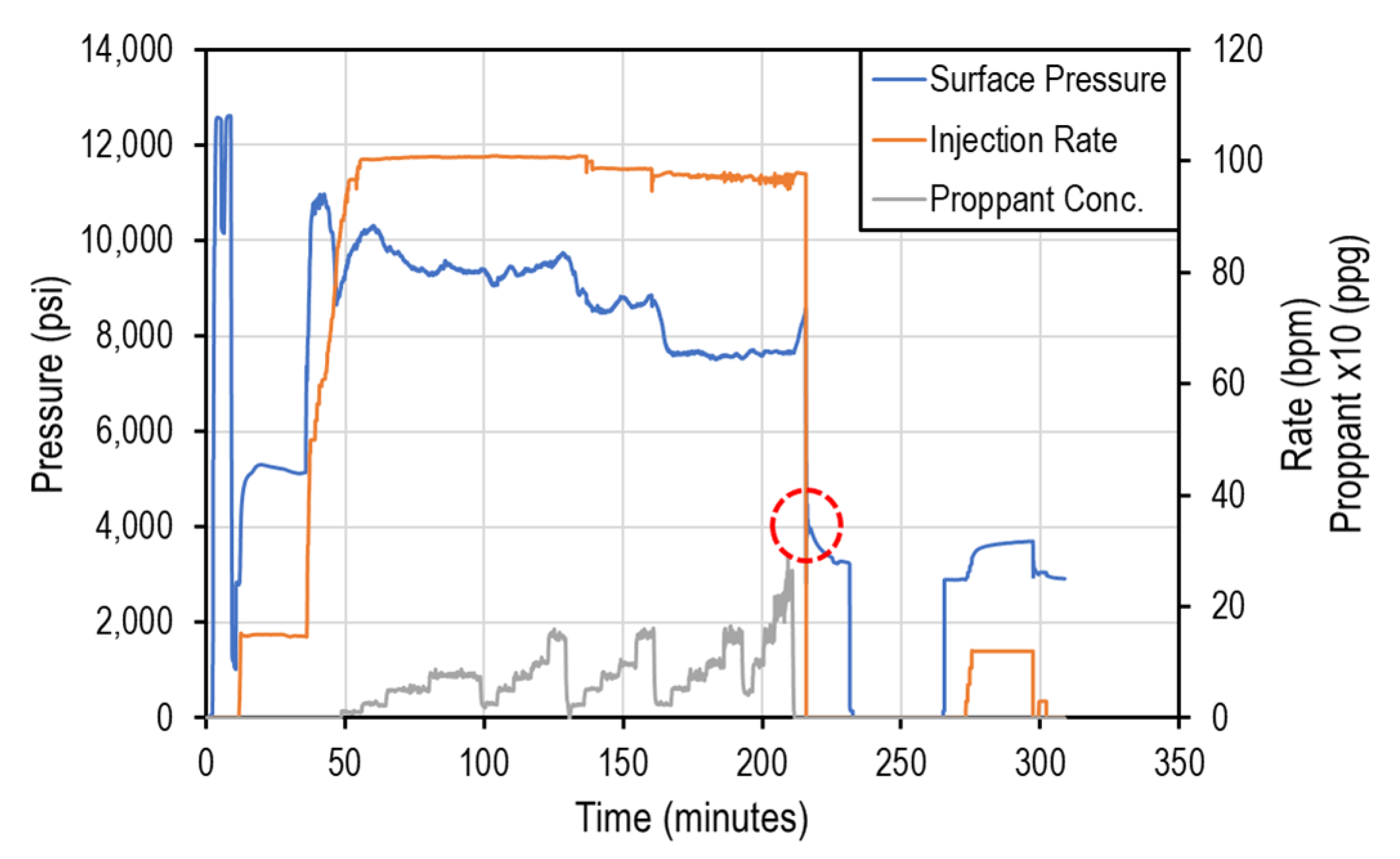
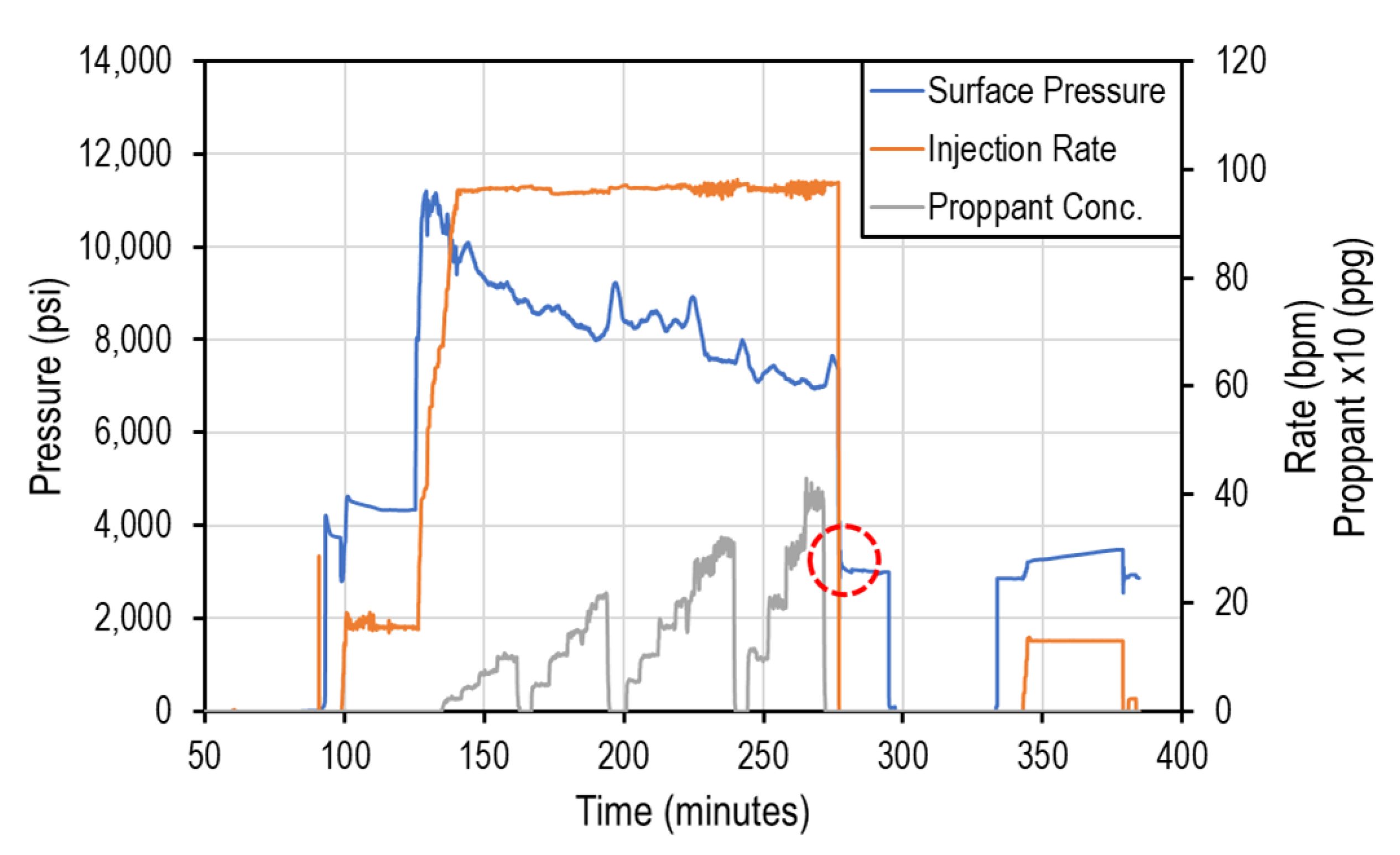


| Parameters | Well #1 | Well #2 |
|---|---|---|
| Lateral length | 10,000 ft | 10,000 ft |
| Stage number | 40 | 36 |
| Cluster/stage | 4 | 5 |
| Cluster spacing | 60 ft | 50 ft |
| Perfs per cluster | 4 | 15 |
| Perf diameter | 0.4 in | 0.4 |
| Total slurry volume | 694,218 bbl | 489,021 bbl |
| Average rate | 100 bpm | 100 bpm |
| Proppant mass and type | 18,966,860 lb (40% 100 mesh, 20% 30/50 premium, 20% 40/70 premium, and 20% 40/70 premium) | 24,675,997 lb (10% 100 mesh, 55% 30/50 premium, 35% 20/40 premium) |
| Time (Days) | Event |
|---|---|
| 0 | Both wells are drilled, and Well #1 is hydraulically fractured |
| 15 | Well #2 is hydraulically fractured |
| 90 | Well #1 is put on production |
| 100 | Well #2 is put on production |
| Half Length (ft) | Height Growth (ft) | ||||
|---|---|---|---|---|---|
| Well | East | West | Upward | Downward | |
| #1 | Minimum | 1154 | 2030 | 547 | 53 |
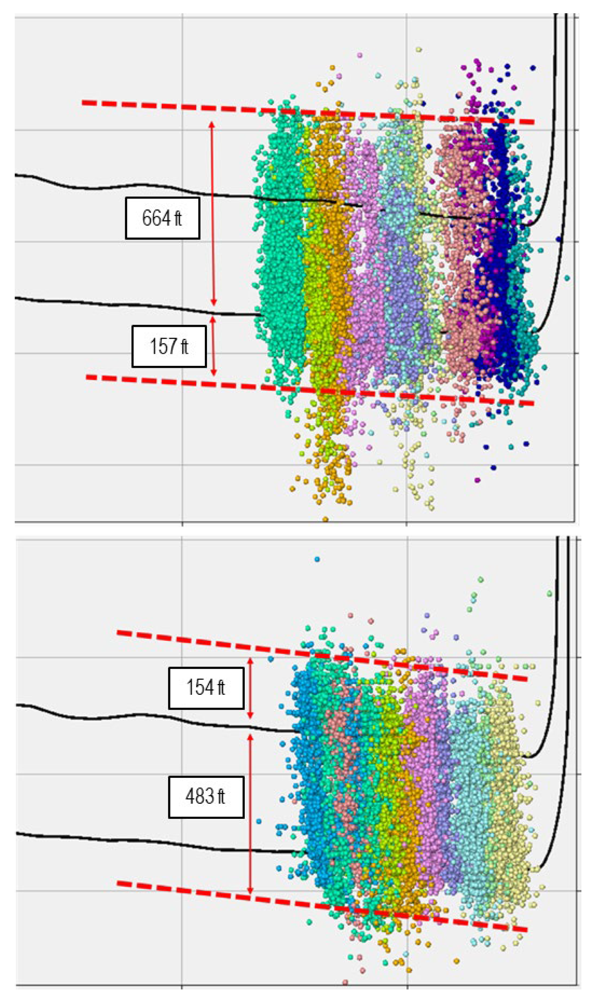
| Average | 1900 | 1620 | 644 | 157 | |
| Maximum | 2554 | 2920 | 744 | 315 | |
| #2 | Minimum | 743 | 1814 | 76 | 345 |
| Average | 1282 | 2173 | 154 | 483 | |
| Maximum | 1982 | 2664 | 214 | 614 | |
Disclaimer/Publisher’s Note: The statements, opinions and data contained in all publications are solely those of the individual author(s) and contributor(s) and not of MDPI and/or the editor(s). MDPI and/or the editor(s) disclaim responsibility for any injury to people or property resulting from any ideas, methods, instructions or products referred to in the content. |
© 2023 by the authors. Licensee MDPI, Basel, Switzerland. This article is an open access article distributed under the terms and conditions of the Creative Commons Attribution (CC BY) license (https://creativecommons.org/licenses/by/4.0/).
Share and Cite
Merzoug, A.; Ellafi, A.; Rasouli, V.; Jabbari, H. Anisortopic Modeling of Hydraulic Fractures Height Growth in the Anadarko Basin. Appl. Mech. 2023, 4, 44-69. https://doi.org/10.3390/applmech4010004
Merzoug A, Ellafi A, Rasouli V, Jabbari H. Anisortopic Modeling of Hydraulic Fractures Height Growth in the Anadarko Basin. Applied Mechanics. 2023; 4(1):44-69. https://doi.org/10.3390/applmech4010004
Chicago/Turabian StyleMerzoug, Ahmed, Abdulaziz Ellafi, Vamegh Rasouli, and Hadi Jabbari. 2023. "Anisortopic Modeling of Hydraulic Fractures Height Growth in the Anadarko Basin" Applied Mechanics 4, no. 1: 44-69. https://doi.org/10.3390/applmech4010004
APA StyleMerzoug, A., Ellafi, A., Rasouli, V., & Jabbari, H. (2023). Anisortopic Modeling of Hydraulic Fractures Height Growth in the Anadarko Basin. Applied Mechanics, 4(1), 44-69. https://doi.org/10.3390/applmech4010004