Towards Ab-Initio Simulations of Crystalline Defects at the Exascale Using Spectral Quadrature Density Functional Theory


National Center for Computational Sciences, Oak Ridge National Laboratory, Oak Ridge, TN 37830, USA
Appl. Mech. 2022, 3(3), 1080-1090; https://doi.org/10.3390/applmech3030061
Submission received: 29 June 2022
/
Revised: 18 August 2022
/
Accepted: 19 August 2022
/
Published: 24 August 2022
(This article belongs to the Special Issue Applied Thermodynamics: Modern Developments)
Abstract
:Defects in crystalline solids play a crucial role in determining properties of materials at the nano, meso- and macroscales, such as the coalescence of vacancies at the nanoscale to form voids and prismatic dislocation loops or diffusion and segregation of solutes to nucleate precipitates, phase transitions in magnetic materials via disorder and doping. First principles Density Functional Theory (DFT) simulations can provide a detailed understanding of these phenomena. However, the number of atoms needed to correctly simulate these systems is often beyond the reach of many widely used DFT codes. The aim of this article is to discuss recent advances in first principles modeling of crystal defects using the spectral quadrature method. The spectral quadrature method is linear scaling with respect to the number of atoms, permits spatial coarse-graining, and is capable of simulating non-periodic systems embedded in a bulk environment, which allows the application of appropriate boundary conditions for simulations of crystalline defects. In this article, we discuss the state-of-the-art in ab-initio modeling of large metallic systems of the order of several thousand atoms that are suitable for utilizing exascale computing resourses.
1. Introduction
Crystal defects, often present in small concentrations, are crucial in determining macroscopic properties of materials. Vacancies are fundamental to creep, spall and radiation aging, even when they are present in parts per million. Solutes, present in parts per hundred, are responsible for strengthening by interacting with the motion of dislocations. Solutes can also cluster to nucleate a precipitate. Dislocations are the primary carriers of plasticity in metals even when their density is as small as per atomic row. Defects not only influence structural properties but also affect electronic and magnetic properties as well. For example, p-type and n-type semiconductors are primarily achieved by dopants. Doping and site mixing by magnetic ions in magnetic compounds can bring about magnetic phase transitions. Defects affect the macroscopic properties of crystals. This is because they simultaneously couple the chemical effects of the defect core, the discrete effects of the lattice and the long range effects of the elastic fields. Thus, to understand defects at physically relevant concentrations, we need to simultaneously study the details near the core and the long range elastic fields.
Density Functional Theory (DFT), developed by Hohenberg, Kohn and Sham [1,2], is one of the most successful first principles methods for predicting, understanding and developing insights into a wide range of material behavior. The phenomenal success and popularity of DFT is because of its excellent predictive power with high accuracy to cost ratio compared to other theories that solve for the electronic structure. In spite of this, the efficient solution of Kohn–Sham equations is computationally daunting, as the computational complexity of DFT calculations scale cubically with the number of atoms N (i.e., ). This restricts the range of physical systems that can be investigated. A number of methods have been proposed that reduce the prefactor by subspace projection [3,4,5,6]. Other methods focus on overcoming the cubic scaling bottleneck which can scale sub-quadratic [7] linear [8,9] and sub-linear [10] with the number of atoms. Methods that solve for orbitals achieve linear scaling by localizing the orbitals in real-space. However this approach only works for insulating or semiconducting systems. Other linear scaling methods do not solve the orbitals, and instead are based on the exponential decay of the density matrix and expand the density matrix using polynomials followed by truncation of off-diagonal components. The primary issue with this type of approach is the complicated interprocessor communication arising from distributed matrix–matrix products with changing sparsity patterns.
The Spectral Quadrature method is an alternative linear scaling formulation [8,10,11,12,13,14,15] suited for first-principles simulations of metallic as well as insulating and semiconducting systems. The key idea of this formulation is to write the electron density and energies as integrals over the spectrum of the linearized Hamiltonian, and then approximate these integrals by quadrature rules. The order of the quadrature is independent of system size, thereby allowing the evaluation of the electron density and energy with effort at each spatial point. The number of spatial points scale linearly with system size, and therefore the method scales linearly. This method has other attractive features as well. First, it allows the application of non-zero Dirichlet boundary conditions on the electronic fields [15]. This is specifically attractive for studying crystalline defects, where periodic boundary conditions can introduce artificial interactions. Second, the local nature of the spectral quadrature calculation allows variable resolution and coarse graining [8,10,14]. Specifically, fine resolution is maintained where necessary and sub-grid sampling is employed in regions of uniform deformation. See Figure 1 for different modeling schemes used for studying defects.
The spectral quadrature method and the coarse grained approximation have been applied to the study of crystal defects [10,14,15], and high temperature simulations of materials [13,19,20]. In this paper, we present an overview of the spectral quadrature formulation and discuss results on defects in magnesium.
2. Spectral Quadrature
In Kohn–Sham Density Functional Theory, the ground state energy () of a system with atomic positions is given by minimizing the Kohn–Sham energy functional over the set of orbitals .
The orbitals are orthonormal, which give rise to the typical cubic scaling of Kohn–Sham DFT. As a consequence of their orthonormality, the orbitals are long ranged, oscillatory and do not decay in metallic systems. Several linear scaling approaches have been developed by localizing or truncating the orbitals in real space. Though these approaches are limited to insulating and semiconducting systems, they do not work for metallic systems i.e., absence of a band-gap. An alternate route is to work with the density operator formulation of DFT. The density operator () is
where are the occupancies of the orbital with energy .
The Kohn–Sham energy functional can be expressed in terms of the density operator, and the ground state energy is then given by minimizing this functional over the density operator.
The diagonal of the density operator is the electron density (i.e., ).
The solution to Equation (3) is given by the following fixed-point problem:
where is the Kohn–Sham Hamiltonian, is the Fermi level, and is the electronic smearing. The right side of Equation (3) can be expanded as a polynomial of , the discrete version of . Linear scaling methods based on the polynomial expansion of are known as Fermi Operator Expansion (FOE), make use of the sparsity, off-diagonal decay of the density operator, and ignore the entries of matrix-matrix products which are lower than a certain tolerance. In large-scale simulations using the FOE method, is distributed across several computational cores, and the global matrix-matrix multiplications with changing sparsity patterns can give rise to complicated parallel communication.
The Spectral Quadrature method [8,10,11,12,13,14,15] is an alternate linear scaling formulation of DFT where the essential ground state quantities are expressed as integrals over the spectrum of the Hamiltonian.
where is the spectrum of , and is the spectral measure of contracted with . The above integral (Equation (5)) can be approximated using quadratures.
where K is the order of the quadrature are the spectral weights and are the spectral nodes. The quadrature order is independent of the system size, hence each evaluation of Equation (6) is . The summation (Equation (6)) is evaluated at every discrete point in real space and the number of such discrete points scale linearly with the number of atoms N, and therefore the scaling of evaluating the ground state is linear.
In spectral Gauss quadrature, the weights are fixed apriori, and the spectral nodes are treated as unknowns. The spectral weights and nodes at any grid point q can be calculated by the Lanczos iteration,
where , , and is computed such that . and are used to construct a tri-diagonal Jacobi matrix , where is the diagonal and are the subdiagonal and superdiagonal entries. The nodes are calculated as the eigenvalues of , and the weights are the squares of the first elements of the normalized eigenvectors of . The Lanczos iteration (Equation (7)) is the most computationally expensive part of the entire computation and can be accelerated by offloading onto Graphics Processing Units (GPUs).
After the spectral weights and spectral nodes are evaluated at a grid point q using the Lanczos scheme (Equation (7)), the electron density at the grid point is given by
The electron density, and similarly other electronic fields, can be calculated in a linear scaling fashion using the spectral quadrature technique. The prefactor can be reduced by noting that the growth of vectors are restricted within a sphere of a finite radius—typically a few lattice spacings—around the grid point q. Therefore, the discrete Hamiltonian in Equation (7), can be spatially truncated beyond a certain distance. This insight allows us to employ local sparse algebra routines instead of distributed sparse algebra, decreases computation time, and storage.
Spatial Coarse Graining
The Spectral Quadrature Method can be used for large scale first principles simulations of materials. Typical calculations with the Spectral quadrature method involve several hundred to tens of thousands of atoms. Further controlled approximations can be introduced which can push the number of atoms even higher using the idea of spatial coarse-graining [8,10,14,21]. This is specifically advantageous for simulating extended defects such as dislocations. To understand heuristics involved in the approximations, first consider an isolated defect. The electronic fields and the atomic displacements are complex in the vicinity of the defect. Moving far away from the defect, the atomic displacements decay in either a polynomial of logarithmic manner, and the electronic fields far away from the defect are almost locally periodic. In the coarse grained formulation, the nature of the decay of the elastic and the electronic fields are exploited in the following manner. First, the position of all atoms is approximated by tracking only a subset of Representative Atoms (RAs) which are fully dense in the vicinity of the defect core and is increasingly sparse with increase in distance from the defect. The positions of atoms which are not in are evaluated by linear interpolation, which provides a coarse grained representation of the atomistic fields. Next, for the electronic fields, the discrete Hamiltonian is defined uniformly on a spatial finite difference mesh . However, the electronic fields are not evaluated at all points in . Instead, a different representation is employed based on the observation that sufficiently far away from the defect, the atom positions are locally periodic, where the periodicity is related to the local strain, and the electronic fields are almost locally periodic. Due to this, the electronic fields can be written as the sum of a corrector and a locally periodic predictor in the following way:
where is the piecewise periodic predictor and is the corrector at a mesh point . The predictor can be calculated by using a periodic DFT calculation with the lattice parameters subjected to local strain. To calculate the corrector, the electron density is first calculated at a select few points using Spectral quadrature, and the difference between the electron density and predictor is interpolated onto the points in :
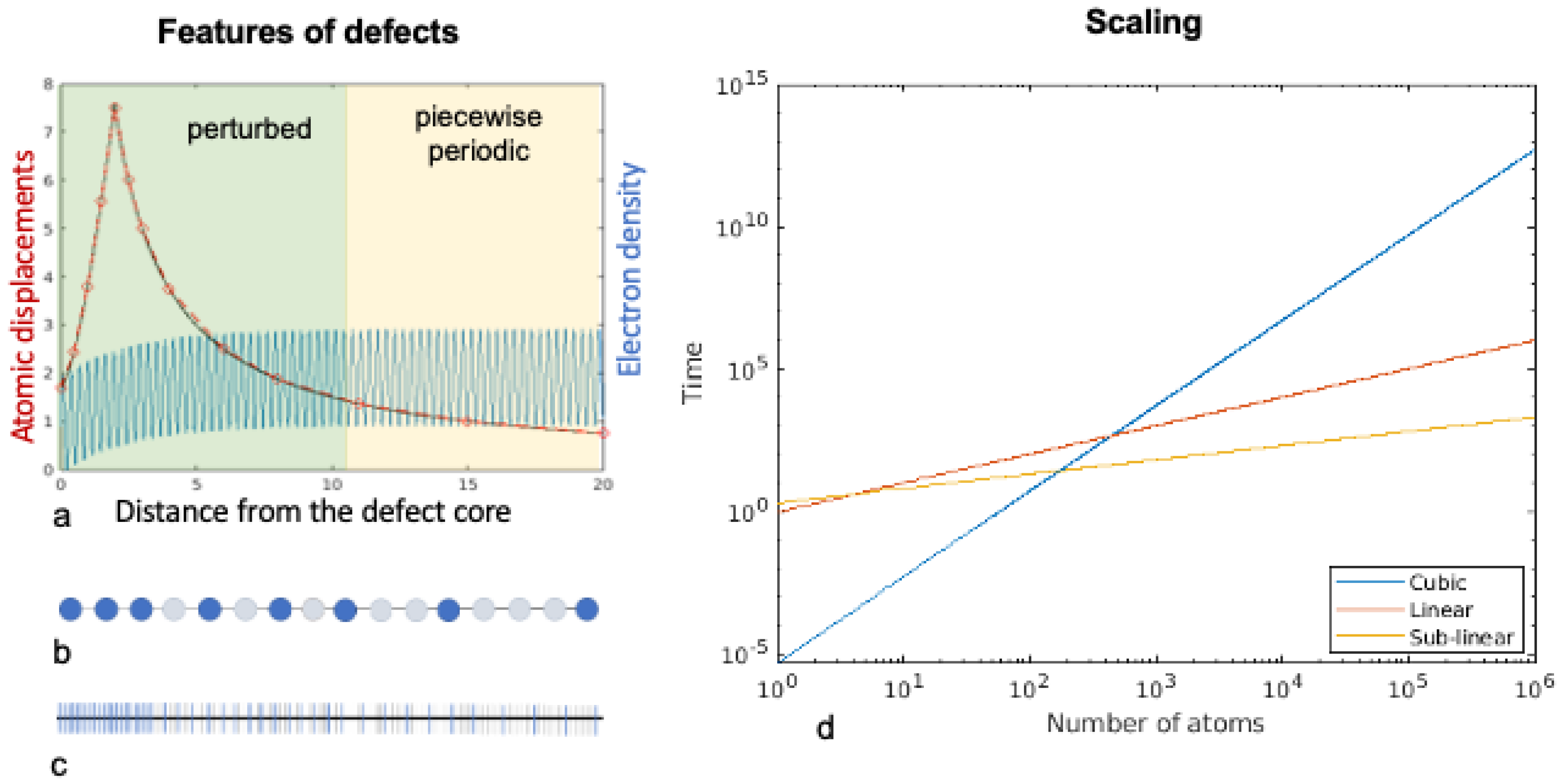
where the is a subset of . Once the electronic fields are calculated, the total energy can be computed using cluster summation technique [22]. Figure 2a–c shows the features of defects and the associated atomic and electronic mesh for a one dimensional system.
Note that, because the electron density is calculated only on a select few points in , the scaling is sub-linear with respect to the total number of atoms in the domain. Figure 2d shows the representative plot of computation time versus number of atoms for cubic, linear and sub-linear scaling methods.
In the coarse-grained formulation, a key computational expense comes from repeated on-the-fly calculation of the predictor electronic fields for every local strain field. This significant overhead can be reduced by employing a neural-network which maps the local strain to the electronic fields. We refer the reader to the recent work by Teh, Ghosh and Bhattacharya [23] for constructing such a map using machine learning.
3. Discussion
3.1. Bulk Properties of Elements
The Spectral Quadrature Method was used to calculate the bulk properties of materials. Higher order finite differences were used to represent the discrete Hamiltonian operator. The finite difference mesh spacing and tolerances were chosen such that the energies and forces are converged to within chemical accuracies. Table 1 shows the values of equilibrium lattice constant and bulk modulus for Li, Na and Mg. Overall, the values calculated using the spectral quadrature DFT are in excellent agreement with the values calculated using DFT, and experiments.
3.2. Defects in Magnesium
Defects in crystalline materials give rise to several interesting phenomena such as creep, spall, plasticity, radiation aging, phase transitions. Defects are present in very small concentrations which make their accurate study challenging. Defect can also interact with other defects in crystalline solids. Vacancies can coalesce to nucleate voids, solutes cluster to nucleate a precipitate, solutes bind to vacancies for diffusion, solutes interact with dislocations for strengthening.
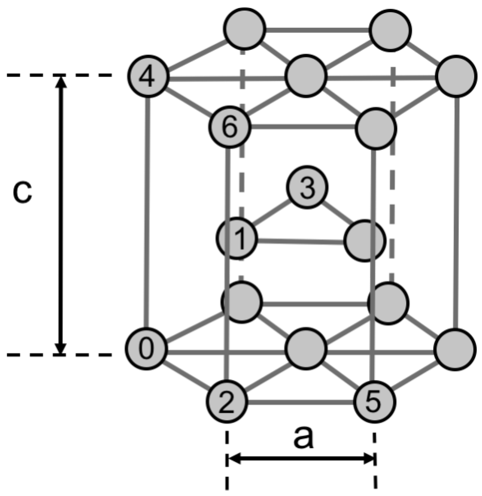
We consider divacancy, solute–vacancy and solute–solute pairs in magnesium lattice. Figure 3 shows the six nearest neighbor positions on a HCP lattice where the first defect is placed at the position marked 0 and the other defect occupies positions marked 1 through 6. These denote the first six nearest neighbor configurations in increasing order of their distances from the defect at position 0. Let , and denote the energies of divacancy, solute–vacancy and solute–solute pairs, respectively in a magnesium supercell with M lattice sites. The formation energies of the divacancy pair is:
where is the energy of a magnesium atom in the perfect crystalline state. The formation energy of the solute–vacancy pair is:
where is the energy of a solute atom in in the perfect crystalline state. The formation energy of the solute–solute pair is:
A negative formation energy implies that the defect formation is energetically favorable.
The binding energy of defect pair can be calculated as the difference between the sum of formation energies of the individual isolated defects and the defect pair.
where and are the formation energies of vacancies and solutes respectively. A positive binding energy implies that the defect pair is more stable than the individual isolated defects.
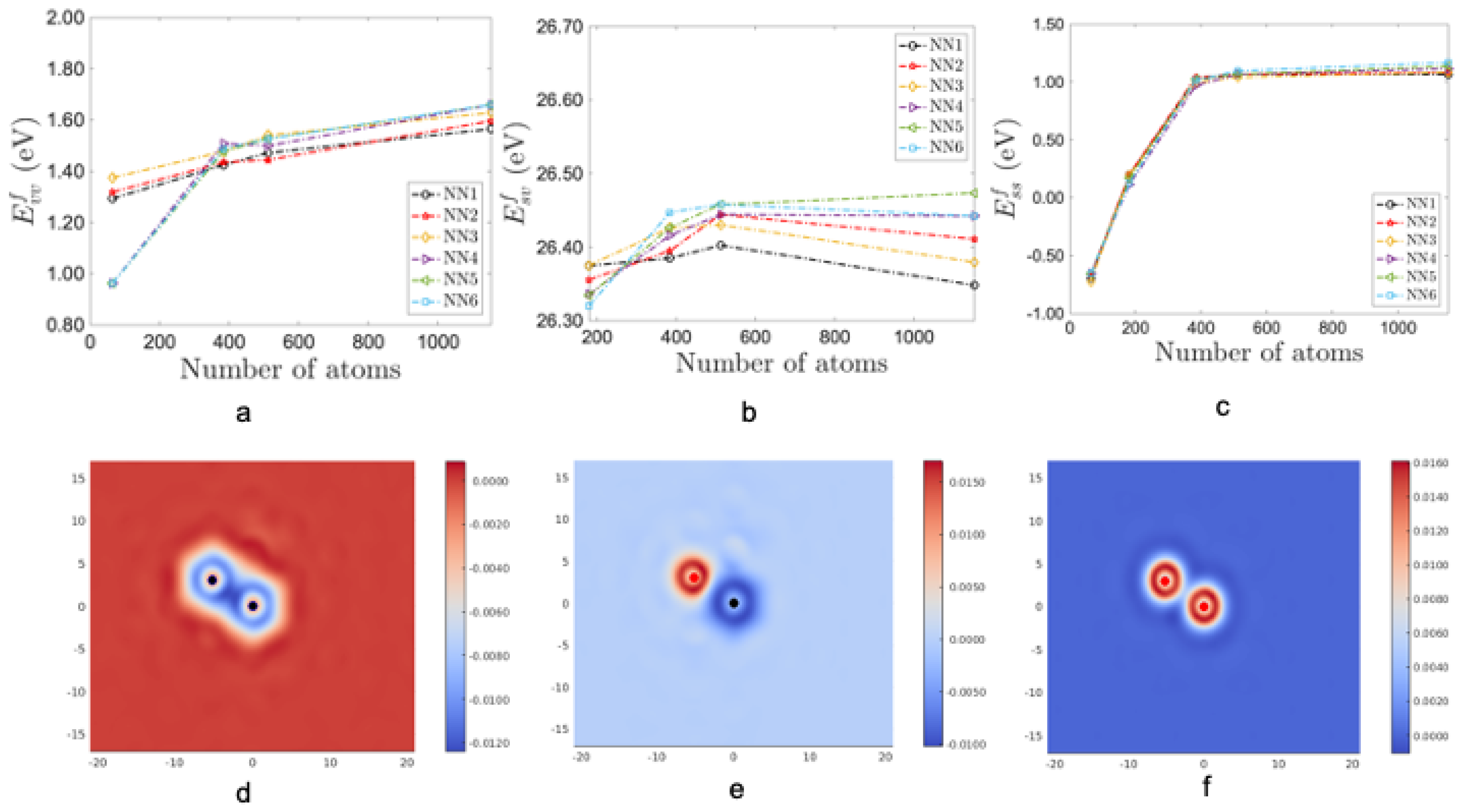
In Figure 4, the top-panel shows the formation energies of (a) divacancy, (b) Al solute–vacancy and (c) Al solute–solute pairs, respectively with increasing cell size from 64 to 1152 atoms. From these plots we see that the formation energy of defect pairs strongly depend on the cell size. Furthermore, the solute–solute formation energy calculated at cell sizes less than 200 atoms is negative but is positive at larger cell sizes. The bottom panel of Figure 4 shows the contours of the difference in electron density of the defect pairs in the second nearest neighbor configuration. We see the depletion of charge around vacancies and an accumulation of charge around the solute atoms.
Table 2 shows the formation and binding energies of isolated defects and defect pairs calculated using the spectral quadrature method. The formation energy of a monovacancy and Al solute is positive. Further the formation energies of divacancy, solute–vacancy and solute–solute pairs are also positive. Interestingly, the formation energy increases from ∼1 eV to ∼26 eV when the system is changed from a divacancy to an Al solute–vacancy pair, but decreases to ∼1 eV for solute–solute pair. Thus, the formation energy follows a non-linear trend with increasing solute number. The equilibrium concentration of spontaneously formed vacancies and divacancies depend on the formation energy and temperature as . As the formation energies of divacancies are greater than monovacancies, the spontaneous formation of monovacancies is favored over the spontaneous formation of divacancies. Additionally, the binding energies of divacancies are positive, implying two monovacancies can coalesce to form a divacancy. Again from Table 2, the binding energies of solute–vacancy and solute–solute pairs are also positive. The solute–vacancy binding energy is also greater than the divacancy binding energy, which implies that solute and vacancy can strongly bind, which aids the self diffusion of solute atoms. As the solute–solute binding energy is also large, these solutes atoms can bind to each other, form clusters and nucleate precipitates [15].
The Spectral Quadrature Method can be used to simulate even larger systems, containing several tens of thousands of atoms. Figure 5 shows the electron density contours around a prismatic dislocation loop in Magnesium calculated using 24,539 atoms, and the prismatic loop consists of a cluster of 37 vacancies. The cell sizes used in these calculations are beyond the scope of most widely popular DFT codes. Calculations with coarse-grained spectral quadrature reveal the preference towards forming large stable vacancy clusters and preference towards forming large prismatic dislocation loops by clustering of vacancies, as observed in nanoporous Mg alloys and experiments [14]. Further optimizing the Lanczos iteration into Graphics Processing Units (GPUs) and utilizing exascale resources (e.g., Frontier) will significantly increase the size of systems to several hundred thousand atoms.
We finally close by commenting on the applicability of the above method to problems in the mechanical behavior of materials. It is of interest to calculate the influence of defects on the mechanical moduli of a crystal. Simulating processes involving material flow [28] and additive manufacturing [29] require accurate estimation of effective moduli of materials under evolving defects such as voids and precipitate growth. Micromechanics approaches dating back to the work of Eshelby [30], Hashin and Shtrikman [31] provide upper and lower bounds on the moduli. Traditional DFT methods have been used to calculate the moduli under high defect concentrations [32]. Therefore, it will be interesting to use the spectral quadrature method on exascale computing resources to calculate the influence of voids and precipitates at high or realistic concentrations from ab-initio.
4. Conclusions
In this article, we discuss recent advances in first principles simulations of bulk materials and crystalline defects using the Spectral Quadrature Computational method. This framework is capable of simulating non-periodic systems embedded in a bulk environment, which allows the application of correct boundary conditions for simulations of crystalline defects. Furthermore, due to the local representation of the electronic fields, this method is also amenable to spatial coarse graining. We have presented studies of defect clusters in magnesium using cell sizes ranging from a few tens to several tens of thousands of atoms. These calculations are typically beyond the reach of the most widely used DFT codes. Due to the local nature of all calculations, the method is amenable to spatial coarse-graining which can be further accelerated by utilizing machine learning models. Furthermore, the local computations can be transferred onto Graphics Processing Units (GPUs), which significantly reduces the solution times. These features make the formulation suitable for efficiently utilizing the exascale supercomputing frameworks.
Funding
Some of the computations were carried out on the Caltech High Performance Cluster partially supported by a grant from the Gordon and Betty Moore Foundation. This research was also funded in part by the NSF-XSEDE and it used resources of the Oak Ridge Leadership Computing Facility, which is supported by the Office of Science of the U.S. Department of Energy under Contract No. DE-AC05-00OR22725.
Institutional Review Board Statement
Not applicable.
Informed Consent Statement
Not applicable.
Data Availability Statement
All data generated or analyzed during this study are included in this published article.
Acknowledgments
This manuscript has been authored in part by UT-Battelle, LLC, under contract DE-AC05-00OR22725 with the US Department of Energy (DOE). The publisher acknowledges the US government license to provide public access under the DOE Public Access Plan (http://energy.gov/downloads/doe-public-access-plan accessed on 29 June 2022).
Conflicts of Interest
The author declare no conflict of interest.
References
- Hohenberg, P.; Kohn, W. Inhomogeneous Electron Gas. Phys. Rev. 1964, 136, B864–B871. [Google Scholar] [CrossRef] [Green Version]
- Kohn, W.; Sham, L.J. Self-Consistent Equations Including Exchange and Correlation Effects. Phys. Rev. 1965, 140, A1133–A1138. [Google Scholar] [CrossRef] [Green Version]
- Zhou, Y.; Saad, Y.; Tiago, M.L.; Chelikowsky, J.R. Parallel self-consistent-field calculations via Chebyshev-filtered subspace acceleration. Phys. Rev. E 2006, 74, 066704. [Google Scholar] [CrossRef] [PubMed] [Green Version]
- Ghosh, S.; Suryanarayana, P. SPARC: Accurate and efficient finite-difference formulation and parallel implementation of Density Functional Theory: Isolated clusters. Comput. Phys. Commun. 2017, 212, 189–204. [Google Scholar] [CrossRef] [Green Version]
- Ghosh, S.; Suryanarayana, P. SPARC: Accurate and efficient finite-difference formulation and parallel implementation of Density Functional Theory: Extended systems. Comput. Phys. Commun. 2017, 216, 109–125. [Google Scholar] [CrossRef] [Green Version]
- Motamarri, P.; Das, S.; Rudraraju, S.; Ghosh, K.; Davydov, D.; Gavini, V. DFT-FE—A massively parallel adaptive finite-element code for large-scale density functional theory calculations. Comput. Phys. Commun. 2020, 246, 106853. [Google Scholar] [CrossRef]
- Motamarri, P.; Gavini, V. Subquadratic-scaling subspace projection method for large-scale Kohn–Sham density functional theory calculations using spectral finite-element discretization. Phys. Rev. B 2014, 90, 115127. [Google Scholar] [CrossRef] [Green Version]
- Suryanarayana, P. On spectral quadrature for linear-scaling Density Functional Theory. Chem. Phys. Lett. 2013, 584, 182–187. [Google Scholar] [CrossRef]
- Bowler, D.; Miyazaki, T. O(N) methods in electronic structure calculations. Rep. Prog. Phys. 2012, 75, 036503. [Google Scholar] [CrossRef]
- Ponga, M.; Bhattacharya, K.; Ortiz, M. A sublinear-scaling approach to density-functional-theory analysis of crystal defects. J. Mech. Phys. Solids 2016, 95, 530–556. [Google Scholar] [CrossRef] [Green Version]
- Suryanarayana, P.; Bhattacharya, K.; Ortiz, M. Coarse-graining Kohn–Sham Density Functional Theory. J. Mech. Phys. Solids 2013, 61, 38–60. [Google Scholar] [CrossRef] [Green Version]
- Pratapa, P.P.; Suryanarayana, P.; Pask, J.E. Spectral Quadrature method for accurate O (N) electronic structure calculations of metals and insulators. Comput. Phys. Commun. 2016, 200, 96–107. [Google Scholar] [CrossRef] [Green Version]
- Sharma, A.; Hamel, S.; Bethkenhagen, M.; Pask, J.E.; Suryanarayana, P. Real-space formulation of the stress tensor for O (N) density functional theory: Application to high temperature calculations. J. Chem. Phys. 2020, 153, 034112. [Google Scholar] [CrossRef] [PubMed]
- Ponga, M.; Bhattacharya, K.; Ortiz, M. Large scale ab-initio simulations of dislocations. J. Comput. Phys. 2020, 407, 109249. [Google Scholar] [CrossRef] [Green Version]
- Ghosh, S.; Bhattacharya, K. Spectral quadrature for the first principles study of crystal defects: Application to magnesium. J. Comput. Phys. 2022, 456, 111035. [Google Scholar] [CrossRef]
- Rao, S.; Hernandez, C.; Simmons, J.; Parthasarathy, T.; Woodward, C. Green’s function boundary conditions in two-dimensional and three-dimensional atomistic simulations of dislocations. Philos. Mag. A 1998, 77, 231–256. [Google Scholar] [CrossRef]
- Trinkle, D.R. Lattice Green function for extended defect calculations: Computation and error estimation with long-range forces. Phys. Rev. B 2008, 78, 014110. [Google Scholar] [CrossRef] [Green Version]
- Sinclair, J.; Gehlen, P.; Hoagland, R.; Hirth, J. Flexible boundary conditions and nonlinear geometric effects in atomic dislocation modeling. J. Appl. Phys. 1978, 49, 3890–3897. [Google Scholar] [CrossRef]
- Suryanarayana, P.; Pratapa, P.P.; Sharma, A.; Pask, J.E. SQDFT: Spectral Quadrature method for large-scale parallel O (N) Kohn–Sham calculations at high temperature. Comput. Phys. Commun. 2018, 224, 288–298. [Google Scholar] [CrossRef] [Green Version]
- Zhang, S.; Lazicki, A.; Militzer, B.; Yang, L.H.; Caspersen, K.; Gaffney, J.A.; Däne, M.W.; Pask, J.E.; Johnson, W.R.; Sharma, A.; et al. Equation of state of boron nitride combining computation, modeling, and experiment. Phys. Rev. B 2019, 99, 165103. [Google Scholar] [CrossRef] [Green Version]
- Gavini, V.; Bhattacharya, K.; Ortiz, M. Vacancy clustering and prismatic dislocation loop formation in aluminum. Phys. Rev. B 2007, 76, 180101. [Google Scholar] [CrossRef] [Green Version]
- Knap, J.; Ortiz, M. An analysis of the quasicontinuum method. J. Mech. Phys. Solids 2001, 49, 1899–1923. [Google Scholar] [CrossRef] [Green Version]
- Teh, Y.S.; Ghosh, S.; Bhattacharya, K. Machine-learned prediction of the electronic fields in a crystal. Mech. Mater. 2021, 163, 104070. [Google Scholar] [CrossRef]
- Fiolhais, C.; Perdew, J.P.; Armster, S.Q.; MacLaren, J.M.; Brajczewska, M. Dominant density parameters and local pseudopotentials for simple metals. Phys. Rev. B 1995, 51, 14001–14011. [Google Scholar] [CrossRef]
- Huang, C.; Carter, E.A. Transferable local pseudopotentials for magnesium, aluminum and silicon. Phys. Chem. Chem. Phys. 2008, 10, 7109–7120. [Google Scholar] [CrossRef]
- Kittel, C. Introduction to Solid State Physics; Wiley: New York, NY, USA, 1976; Volume 8. [Google Scholar]
- Koster, W.; Franz, H. Poisson’s ratio for metals and alloys. Metall. Rev. 1961, 6, 1–56. [Google Scholar] [CrossRef]
- Tamadon, A.; Pons, D.J.; Clucas, D. Flow-Based Anatomy of Bobbin Friction-Stirred Weld; AA6082-T6 Aluminium Plate and Analogue Plasticine Model. Appl. Mech. 2020, 1, 3–19. [Google Scholar] [CrossRef] [Green Version]
- Du Plessis, A.; Yadroitsava, I.; Yadroitsev, I. Effects of defects on mechanical properties in metal additive manufacturing: A review focusing on X-ray tomography insights. Mater. Des. 2020, 187, 108385. [Google Scholar] [CrossRef]
- Eshelby, J.D. The determination of the elastic field of an ellipsoidal inclusion, and related problems. Proc. R. Soc. Lond. Ser. A Math. Phys. Sci. 1957, 241, 376–396. [Google Scholar]
- Hashin, Z.; Shtrikman, S. A variational approach to the theory of the elastic behaviour of multiphase materials. J. Mech. Phys. Solids 1963, 11, 127–140. [Google Scholar] [CrossRef]
- Ghosh, S.; Bhattacharya, K. Influence of thermomechanical loads on the energetics of precipitation in magnesium aluminum alloys. Acta Mater. 2020, 193, 28–39. [Google Scholar] [CrossRef] [Green Version]
Figure 1.
Modeling schemes and boundary conditions used for studying defects in crystalline solids. (a) shows dipolar and (b) shows a quadrapolar arrangement of defects. In both (a,b), periodic boundary conditions are used. (c) shows the schematic of the flexible boundary condition technoque used to simulate dislocations [16,17,18]. (d) shows the specified Dirichlet boundary conditions in the spectral quadrature method. In (d), the inner box is the simulation domain, and the region outside is used to specify pre-computed electronic fields. (e) shows the spatial coarse-grained atomic mesh [14]. The region close to the defect has full atomic resolution, and the resolution is gradually decreased with distance increasing from the defect core.
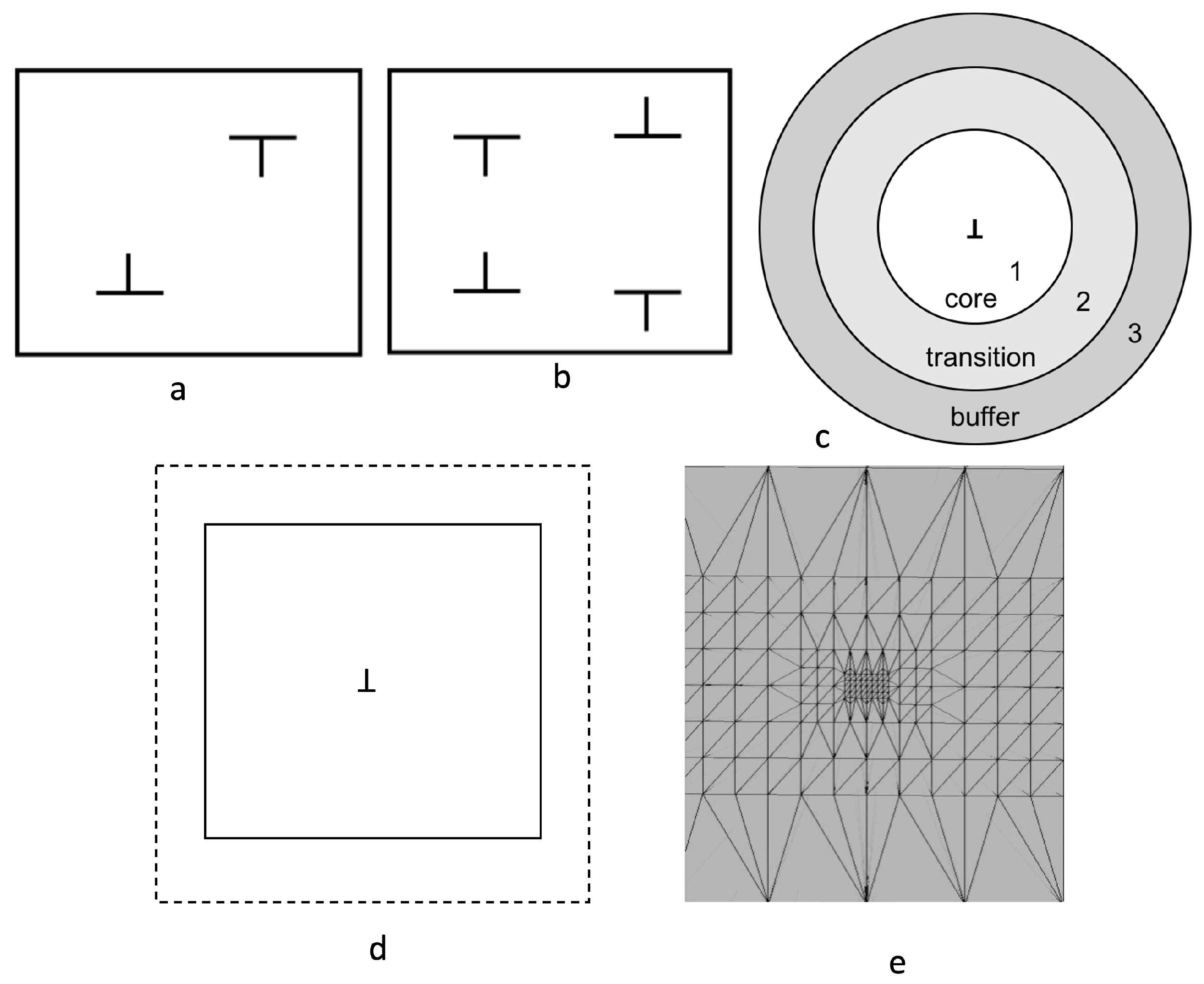
Figure 2.
(a) Shows some features of defects; (b) shows the atomic mesh; and (c) shows the electronic mesh. As depicted in (a) the atomic displacements are complex near the defect but have a polynomial decay far away from the defect. The black line shows the displacement field of the atoms, and the red points are the displacements evaluated on a mesh which is fine resolution near the defect and increasingly coarse further away as shown in (b). The electronic field, shown in blue, is strongly perturbed near the defect and is piecewise periodic far away. The electronic field is evaluated on a mesh that is fine near the defect and increasingly coarse far away as shown by the blue lines in (c). The Hamiltonian operator necessary to evaluate the electronic fields is defined on the uniformly fine mesh shown by the grey lines in (c). (d) shows the scaling of different formulations of DFT. The blue line shows cubic scaling associated with standard DFT formulations. The red line shows the linear scaling associated with the spectral quadrature formulation and the yellow line shows the sub-linear scaling associated with coarse-graining. The lower computation time of linear and sub-linear scaling methods over cubic scaling methods is typically observed for systems larger than a few hundred to thousand atoms.

Figure 3.
Nearest neighbor positions for two point defects in an HCP lattice.

Figure 4.
Formation energy of defect pairs as shown in (a–c). (d–f) shows the contour plots of electron density difference for defect pairs in second nearest neighbor configuration. A cell size of 1000 atoms is needed to calculate the formation energy of defect pairs. The electron density difference around a divacancy is shown in (d), around a Al solute–vacancy pair in (e) and around a Al solute pair in (f). In these plots, the electron density is depleted around a vacancy and elevated near the Al solute.

Figure 5.
Contours of electron density around a prismatic dislocation loop in Mg. The slice is along the a-b plane. The prismatic loop is formed by a cluster of 37 vacancies. The total number of atoms in the simulation domain is 24,539.
Figure 5.
Contours of electron density around a prismatic dislocation loop in Mg. The slice is along the a-b plane. The prismatic loop is formed by a cluster of 37 vacancies. The total number of atoms in the simulation domain is 24,539.


Table 1.
Bulk properties of elements.
| Element | Crystal Structure | Method | Lattice Constant (a.u.) | Bulk Modulus (GPa) |
|---|---|---|---|---|
| Li | BCC | SQ [11] | 6.87 | 10.0 |
| DFT [24] | 6.77 | 14.0 | ||
| Expt. [24] | 6.77 | 13.3 | ||
| Na | BCC | SQ [11] | 8.01 | 5.0 |
| DFT [24] | 8.21 | 7.1 | ||
| Expt. [24] | 8.21 | 7.3 | ||
| Mg | HCP | SQ [10] | 5.866, 1.626 | 38.75 |
| SQ [15] | 6.043, 1.629 | 38.50 | ||
| DFT [25] | 5.877, 1.624 | 38.40 | ||
| Expt. [26,27] | 6.066, 1.623 | 35.40 |
Table 2.
Formation energies of vacancy and Al solute in Mg lattice in eV. Formation and binding energies of divacancies, Al solute–vacancy and Al solute–solute pairs in Mg in eV. First six nearest neighbors are considered for calculation of defect pair binding energies as shown in Figure 3. The cell size used for all calculations is more than 1100 atoms.
| Isolated Defects | |||
|---|---|---|---|
| Formation Energy (eV) | |||
| Vacancy | 0.846 | ||
| Al solute | 25.756 | ||
| Defect Pairs | |||
| Nearest Neighbor | Formation Energy (eV) This Work | Binding Energy (eV) Ref. [15] | |
| Divacancy | 1 | 1.565 | 0.127 |
| 2 | 1.596 | 0.195 | |
| 3 | 1.627 | 0.064 | |
| 4 | 1.659 | 0.033 | |
| 5 | 1.659 | 0.033 | |
| 6 | 1.659 | 0.033 | |
| solute-vacancy | 1 | 25.956 | 0.254 |
| 2 | 26.583 | 0.195 | |
| 3 | 26.583 | 0.206 | |
| 4 | 26.722 | 0.125 | |
| 5 | 26.722 | 0.125 | |
| 6 | 26.722 | 0.125 | |
| solute-solute | 1 | 1.066 | 0.238 |
| 2 | 1.081 | 0.223 | |
| 3 | 1.084 | 0.219 | |
| 4 | 1.112 | 0.191 | |
| 5 | 1.134 | 0.169 | |
| 6 | 1.166 | 0.138 | |
Publisher’s Note: MDPI stays neutral with regard to jurisdictional claims in published maps and institutional affiliations. |
© 2022 by the author. Licensee MDPI, Basel, Switzerland. This article is an open access article distributed under the terms and conditions of the Creative Commons Attribution (CC BY) license (https://creativecommons.org/licenses/by/4.0/).
Share and Cite
MDPI and ACS Style
Ghosh, S. Towards Ab-Initio Simulations of Crystalline Defects at the Exascale Using Spectral Quadrature Density Functional Theory. Appl. Mech. 2022, 3, 1080-1090. https://doi.org/10.3390/applmech3030061
AMA Style
Ghosh S. Towards Ab-Initio Simulations of Crystalline Defects at the Exascale Using Spectral Quadrature Density Functional Theory. Applied Mechanics. 2022; 3(3):1080-1090. https://doi.org/10.3390/applmech3030061
Chicago/Turabian StyleGhosh, Swarnava. 2022. "Towards Ab-Initio Simulations of Crystalline Defects at the Exascale Using Spectral Quadrature Density Functional Theory" Applied Mechanics 3, no. 3: 1080-1090. https://doi.org/10.3390/applmech3030061